An asteroseismic study of the Cephei star 12 Lacertae: multisite spectroscopic observations, mode identification and seismic modelling
Abstract
We present the results of a spectroscopic multisite campaign for the Cephei star 12 (DD) Lacertae. Our study is based on more than thousand high-resolution high S/N spectra gathered with 8 different telescopes in a time span of 11 months. In addition we make use of numerous archival spectroscopic measurements. We confirm 10 independent frequencies recently discovered from photometry, as well as harmonics and combination frequencies. In particular, the SPB-like g-mode with frequency 0.3428 reported before is detected in our spectroscopy. We identify the four main modes as , , and for , , and , respectively. Our seismic modelling shows that is likely the radial first overtone and that the core overshooting parameter is lower than 0.4 local pressure scale heights.
Keywords:
stars: main-sequence – stars: individual: 12 Lac – stars: oscillations – stars: interiors1 Introduction
12 (DD) Lacertae (12 Lac) is one of the best observed Cephei stars, a class of variable early B-type stars whose light and radial velocity changes are due to gravity and pressure-mode pulsations of low radial order (Stankov & Handler, 2005). The variability of 12 Lac has been known for one century during which the star has been extensively studied. We refer to Handler et al. (2006) for a very detailed summary of the work accomplished in the past.
Despite the numerous earlier studies, safe mode identification of the observed modes was not achieved until recently. Thanks to an intensive photometric multisite campaign, Handler et al. (2006) unambiguously identified the -values of the five modes with the highest photometric amplitudes. In addition, they found constraints on for the six other independent modes detected in their dataset. Their -identifications ruled out the assumption previously adopted for stellar modelling (Dziembowski & Jerzykiewicz, 1999, e.g.) that three of the strongest modes, almost equidistant, belong to the same multiplet. Indeed, these three modes are actually associated to three different values of the degree .
Obviously, reliable empirical mode identification was indispensable before any attempt of in-depth seismic modelling of 12 Lac. To complement the photometric results, a spectroscopic multisite campaign has also been devoted to the star. The additional constraints are presented in this paper. They mainly concern the identification of -values for the strongest modes and the derivation of the stellar equatorial velocity. A detailed abundance analysis of 12 Lac was already presented in Morel et al. (2006), showing that the abundances of all considered chemical elements are indistinguishable from the values found for OB dwarfs in the solar neighbourhood.
Besides our line-profile study, we also describe a detailed stellar modelling based on all available observational results, state-of-the-art numerical tools and up-to-date physical inputs appropriate to model Cephei stars, as explained in detail in Miglio (2007). Dziembowski & Pamyatnykh (2008) already computed models for 12 Lac, making some assumptions and restrictions not supported by our study. In the present paper, we discuss our conclusions which differ from those of Dziembowski & Pamyatnykh (2008).


2 Observations and data reduction
The data originate from a spectroscopic multisite campaign dedicated to our studied star. In addition, we added the 903 spectra of Mathias et al. (1994), which allowed us to increase the time span and, thus, to achieve a better frequency accuracy. In total 1820 observations were gathered using 9 different small- to medium-sized telescopes spread over the northern continents. Table 1 summarizes the logbook of our spectroscopic data. The resolution () of the instruments ranged from 30 000 to 80 000 and the average S/N ratio near 4500 Å between 180 and 380.
| Observatory | Long. | Lat. | Telescope | Julian Date | Data amount and quality | Observer(s) | |||
| (Name of the instrument; resolution) | Begin | End | N | S/N | |||||
| 2003-2004 | -2450000 | ||||||||
| Apache Point Observatory | 3.5-m | 2927 | 2928 | 2 | 93 | 300 | JK | ||
| (ARC; 31500) | |||||||||
| Bohyunsan Astronomical Observatory | 1.9-m | 3109 | 3109 | 1 | 27 | 180 | DM | ||
| (BOES; 30000) | |||||||||
| Dominion Astrophysical Observatory | 1.2-m | 2858 | 2859 | 2 | 66 | 250 | SY | ||
| (45000) | 2909 | 2911 | 3 | 42 | |||||
| McDonald Observatory | 2.1-m | 2893 | 2901 | 9 | 210 | 380 | GH | ||
| (Sandiford; 60000) | 2.7-m | 3195 | 3198 | 4 | 31 | 350 | GH | ||
| Nordic Optical Telescope | 2.6-m | 2947 | 2951 | 5 | 32 | 370 | KU, JT, II | ||
| (SOFIN; 80000) | 2957 | 2960 | 4 | 47 | |||||
| Okayama Astrophysical Observatory | 1.88-m | 3201 | 3202 | 2 | 7 | 180 | SM | ||
| (HIDES; 685000) | 3205 | 3205 | 1 | 6 | |||||
| 3208 | 3210 | 3 | 17 | ||||||
| Thüringer Landessternwarte Tautenburg | 2-m | 2863 | 2869 | 7 | 103 | 240 | HL | ||
| (67000) | 2886 | 2889 | 4 | 100 | |||||
| 2895 | 2900 | 6 | 105 | ||||||
| 2914 | 2918 | 5 | 31 | ||||||
| 1990-1992 | -2440000 | ||||||||
| Observatoire de Haute-Provence | 1.52-m | 8135 | 8135 | 1 | 70 | 220 | PM | ||
| (AURELIE; 42000) | 8224 | 8224 | 1 | 52 | |||||
| 8227 | 8227 | 1 | 35 | ||||||
| 8845 | 8858 | 14 | 582 | ||||||
| 8884 | 8889 | 6 | 164 | ||||||
| Total | 82 | 1820 | |||||||
All data were subjected to the normal reduction process, which consists of de-biasing, background subtraction, flat-fielding and wavelength calibration . Finally, the heliocentric corrections were computed, and all spectra were normalized to the continuum by fitting a cubic spline function.
For our study, we considered the Si iii triplet around 4567 Å because its characteristics simplify the modelling of the line-profile variations, which we use for mode identification. Indeed, these silicon lines are sufficiently strong without being much affected by blending. Moreover, they are dominated by temperature broadening, such that the intrinsic profile can simply be modelled with a gaussian. Finally, they are not too sensitive to temperature variations (De Ridder et al., 2002; Aerts & De Cat, 2003, see), so that neglecting them remains justified.
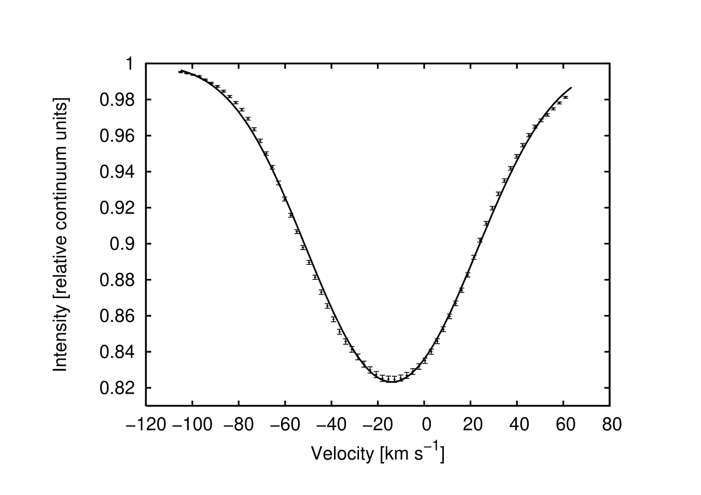
The similar average radial velocity of about for 1990-1992, 2003-2004 and earlier measurements (Wilson, 1953, e.g.) definitely excludes the possibility of 12 Lac being a spectroscopic binary. Besides the pulsation effect, the different centroids are due to the different zero points of the different telescopes. Before extracting the pulsation information from the whole dataset, it is necessary to correct for this effect. The spectra were shifted in such a way that the constant of a least-squares sine fit using the first three dominant modes is put to the same value for each observatory.
In Fig. 1 we superimpose the average profiles of the Si iii Å line computed for each observatory separately, after correction for the different zero points. We note that the centroid of the lines are in good agreement but not exactly at the same position. Larger differences can be seen for the width and the depth of the lines. Such deviant average profiles are due to the limited time spread of the observations together with the multiperiodic character of the pulsations. In the case of a similar spectroscopic multisite campaign devoted to Eridani, Aerts et al. (2004) observed similar differences, which are not caused by instrumental and/or signal-to-noise ratio effects.
Fig. 2 displays the large and complex radial-velocity variations of 12 Lac. The plotted spectra were taken with the McDonald telescope during only one night. In Fig. 3, we show the radial velocities for the densest part of the multisite campaign (7 Aug. 2003 – 17 Nov. 2003). A clear beating pattern is seen.
3 Frequency analysis
We performed a frequency analysis on the first three velocity moments , and (see Aerts et al., 1992, for a definition of the moments of a line profile) of the Si iii Å line by means of the program Period04 (Lenz & Breger, 2005). For some Cephei stars (Telting et al., 1997; Schrijvers et al., 2004; Briquet et al., 2005, see) a two-dimensional frequency analysis on the spectral lines led to additional frequencies compared to a one-dimensional frequency search in the moments. For 12 Lac 1D analysis on and did not reveal additional independent periodicities compared to those present in the first moment. We also do not find additional frequencies in the 2D frequency analysis. The 2D analysis is more sensitive to the detection of high-degree modes than a 1D analysis so here we have already an indication that the frequencies are low-degree modes.
In what follows we only describe our frequency analysis on , which is the radial velocity from which the fitted averaged radial velocity is subtracted.
The frequencies were determined with the standard method of prewhitening the data. In addition we made use of a procedure available in Period04 which allows to improve the detected frequency from non-linear least-squares fitting with the maxima in the Fourier transform as starting values. At each step of prewhitening we subtracted a theoretical multi-sine fit with the amplitudes, phases and also optimized frequencies that yielded the smallest residual variance. All peaks exceeding an amplitude signal-to-noise ratio above 4 in the Fourier periodogram (Breger et al., 1993; Breger et al., 1999) were retained. The noise level was calculated from the average amplitude, computed from the residuals, in a 2 interval centered on the frequency of interest.
| ID | Frequency | Amplitude in | S/N | |
|---|---|---|---|---|
| [ ] | [ ] | [ ] | ||
| 5.178964 | 59.941713 | 14.50 | 99.6 | |
| 5.334224 | 61.738704 | 7.70 | 52.2 | |
| 5.066316 | 58.637917 | 6.26 | 42.7 | |
| 5.490133 | 63.543206 | 2.61 | 17.5 | |
| 0.342841 | 3.968067 | 1.34 | 7.1 | |
| 4.241787 | 49.09475 | 0.91 | 6.7 | |
| 5.218075 | 60.394387 | 0.84 | 5.8 | |
| 6.702318 | 77.573125 | 0.62 | 4.4 | |
| 7.407162 | 85.731042 | 0.67 | 4.9 | |
| 5.84511 | 67.65184 | 0.79 | 5.2 | |
| 10.35814 | 119.88590 | 0.63 | 4.5 | |
| 10.40056 | 120.37693 | 0.72 | 3.8 | |
| 10.51319 | 121.68044 | 2.59 | 19.7 | |
| 15.42400 | 178.51860 | 0.72 | 6.6 | |
| 15.57950 | 180.31838 | 0.71 | 6.4 | |

The detected frequencies are listed in Table 2 and the Fourier periodograms are shown in Fig. 4. Our frequency analysis reaffirmes the presence of the already well-known 5 main frequencies (Mathias et al., 1994) together with the new independent signals and combination frequencies discovered by Handler et al. (2006). We note that one additional independent frequency ( ) was found by the latter authors and not by us. An important result is that we clearly recover the low-frequency signal possibly originating from a -mode. Such a SPB-like oscillation does not seem to be uncommon among Cephei stars. For instance, it was also observed in 19 Mon (Balona et al., 2002), in Eridani (Handler et al., 2004), in Ceti (Aerts et al., 2006) and in V1449 Aql (Briquet et al., in preparation). We also point out that such hybrid SPB- Cep pulsators are theoretically predicted for hotter stars than previously thought (Miglio et al., 2007 versus Pamyatnykh, 1999).
The equivalent width (EW) of the silicon line of 12 Lac clearly varies with the two dominant modes and . The sum frequency is even present. Fig. 5 represents phase diagrams for both frequencies. Such a strong EW variability of is generally not observed in pulsating B-type stars. Indeed, typical relative EW peak-to-peak amplitudes are of the order of a few percent (De Ridder et al., 2002; De Cat & Aerts, 2002). However, for several Cephei stars, one clear sinusoidal variation is observed in their EW, with the same frequency as in the radial velocity. The known cases are targets pulsating multiperiodically with a high-amplitude dominant radial mode, such as Ceti (Aerts et al., 1992), Eridani (Aerts et al., 2004) and V1449 Aql (Briquet et al., in preparation). In the case of 12 Lac, we note that the EW signal is multiperiodic with a dominant -mode, followed by a radial mode of lower amplitude (see next section). For the four strongest modes, the frequency values derived from our spectroscopic measurements are exactly the same, within the errors, as the photometric ones by Handler et al. (2006). For the modes with radial velocity amplitudes typically lower than 1 , there are differences between values derived from both kinds of data, which might have some influence on the mode identification outcome. Because the number of observations as well as the time span of the datasets in the literature are much larger than the dedicated spectroscopic ones, the literature frequency values are expected to be more accurate and hence we adopt them.
4 Mode identification
4.1 The methods used
We used two different and independent methods to identify the modes, namely the moment method (Briquet & Aerts, 2003) and of the Fourier parameter fit method (Zima, 2006, FPF method,).
The basic principles of both methods are the following. With the moment method the wavenumbers and the other continuous velocity parameters are determined in such a way that the theoretically computed first three moment variations of a line profile best fit the observed ones. In the FPF method, for every detected pulsation frequency, the zero point, amplitude, and phase are computed for every wavelength bin across the profile by a multi-periodic least-square fit. Subsequently the zero-point profile, the amplitude and the phase values across the profile are fitted with theoretical values derived from synthetic line profiles. The first technique has the advantage to be less computationally demanding, allowing to test a huge grid for and for the other parameters. Moreover, the modes are determined simultaneously by fitting a multiperiodic signal taking into account the coupling terms appearing in the second and third moments. For the second technique, the fitting is carried out by applying genetic optimization routines in a large parameter space and mono-mode fits are used in order to speed up the computations. Once the best solutions are constrained, a multi-mode fit is performed. The strength of the FPF method is its ability to estimate the significance of the derived mode parameters by means of a test (Zima, 2008, all -values listed in the text are reduced values, see).
The FPF method is not optimally suited to study high-amplitude modes, but as described further, the application of the FPF method for 12 Lac proved to be succesful. As shown by Zima et al. (2004) and by Zima (2006), both mode identification techniques constrain the value of the azimuthal number better than the degree for low . Since the photometric data provided us with unambiguous -values for the 5 main modes (Handler et al., 2006), a valid strategy is to make use of spectroscopy to identify the values of , adopting the -values obtained from photometry. Such a methodology already proved to be successful for two other Cephei stars (Briquet et al., 2005; Mazumdar et al., 2006). Mode identification results have been obtained with the software package FAMIAS11 1 FAMIAS has been developed in the framework of the FP6 European Coordination Action HELAS - http://www.helas-eu.org/. (Zima, 2008).
In what follows we present in detail our mode identification by the FPF method. The moment method gave compatible results, but did not give additional constraints on the than the ones we present here. Both techniques found the same -values for the three main modes, giving us much confidence in our outcome. For the fourth mode, the moment method derived the sign of in agreement with the FPF method, which could further constrain its value.


4.2 Derivation of the wavenumbers
For the FPF method, a sophisticated theoretical formalism for the modelling of the displacement field is used and includes, for instance, first-order effects of the Coriolis force as well as temperature variations of the stellar atmosphere. We refer to Zima (2006); Zima (2008) for details on the computation of the synthetic line-profile variations. The fixed parameters are the mass and the radius. When taking into account temperature effects, the effective temperature and the logarithm of the gravity have also to be fixed. For 12 Lac, we adopted the values (Handler et al., 2006), (Handler et al., 2006), (Morel et al., 2006), (Morel et al., 2006). We note that the mode identification results are robust when using different values for these parameters, within the errors.
In a first step we identified the 3 main modes () by fitting mono-mode Fourier parameters, which are computed from synthetic line profiles evenly sampled over one pulsation cycle (Zima, 2006, for more explanations see). Moreover, we neglected the equivalent width variations of the spectral line due to temperature variations. In order to restrict the parameter space, we estimate roughly the values of the projected rotational velocity , the width of the intrinsic gaussian profile , and the equivalent width from a least-squares fit of a rotationally broadened synthetic profile to the zero-point profile. This gives only a crude estimate of these three parameters, because the pulsational broadening is ignored in this fit, but it serves the purpose of defining our appropriate grid. Moreover will be overestimated. When taken into account the pulsational broadening caused by the four main modes we acquire a of 36.7 (see Fig. 6). A genetic optimization with the following free parameters was afterwards adopted: with a step of 1, with a step of 1, the surface velocity amplitude with a step of 1 , the stellar inclination angle with a step of , with a step of 0.5 and with a step of 0.1 . We fixed as a radial mode and only fitted the continuous parameters for that mode.
| = 5.178964 | = 5.066316 | ||||||||||||
| [ ] | [∘ ] | [ ] | [ ] | [ ] | [∘ ] | [ ] | [ ] | ||||||
| 15.29 | 1 | 1 | 68.7 | 74.6 | 46.47 | 21.00 | 10.34 | 1 | 0 | 24.8 | 59.1 | 42.69 | 26.23 |
| 15.30 | 1 | 1 | 64.9 | 85.0 | 38.15 | 27.82 | 10.38 | 1 | 0 | 24.2 | 59.2 | 42.70 | 26.23 |
| 15.31 | 1 | 1 | 48.2 | 72.1 | 43.72 | 21.64 | 10.39 | 1 | 0 | 25.0 | 51.5 | 42.38 | 26.24 |
| 15.32 | 1 | 1 | 72.3 | 51.4 | 36.03 | 28.62 | 10.40 | 1 | 0 | 26.4 | 48.9 | 42.38 | 26.35 |
| 15.33 | 1 | 1 | 50.9 | 59.2 | 42.00 | 22.58 | 10.41 | 1 | 0 | 25.7 | 59.2 | 43.02 | 26.41 |
| 31.62 | 1 | 0 | 68.4 | 41.2 | 30.79 | 26.66 | 25.99 | 1 | 1 | 18.0 | 74.6 | 43.65 | 26.70 |
| = 5.3324224 | = 5.490133 | ||||||||||||
| [ ] | [∘ ] | [ ] | [ ] | [ ] | [∘ ] | [ ] | [ ] | ||||||
| 12.36 | 0 | 0 | 41.6 | - | 43.65 | 25.17 | 7.73 | 2 | 1 | 26.2 | 15.3 | 40.15 | 27.23 |
| 12.83 | 0 | 0 | 37.0 | - | 36.66 | 28.11 | 7.76 | 2 | 1 | 26.2 | 12.7 | 40.16 | 27.17 |
| 13.07 | 0 | 0 | 42.6 | - | 43.33 | 25.00 | 7.77 | 2 | 1 | 26.2 | 12.7 | 40.79 | 26.76 |
| 13.53 | 0 | 0 | 33.4 | - | 40.47 | 26.41 | 7.79 | 2 | 1 | 27.1 | 12.7 | 40.79 | 27.11 |
| 13.68 | 0 | 0 | 33.3 | - | 44.60 | 24.70 | 7.83 | 2 | 1 | 24.2 | 12.8 | 42.38 | 26.35 |
| 43.68 | 2 | 2 | 23.7 | 82.4 | 41.76 | 26.26 | |||||||
In Table 3, the 5 best solutions from a fit to the Fourier parameters are listed for each frequency. The 95%-confidence limit of is 1.15. The most probable solutions are , and (where a positive -value denotes a prograde mode). We point out that the agreement between theory and observations is not perfect. More precisely, the observed asymmetry with respect to the centroid of the amplitudes across the line of the dominant modes is not completely reproduced by our model. Such an asymmetry can be caused by EW variations of the intrinsic line profile due to local temperature variations (Schrijvers & Telting, 1999). We considered EW variations in our fitting procedure but we did not obtain an improved solution compared to the case of a constant EW.
In a second step we attempted to improve the solutions by simultaneously fitting the four main modes and using all the original data points. This however was computationally not possible. To restrict the computation time we took a subset of our complete time series. Our subset resulted in 388 spectra with a time span of 4 months. We also fixed the wave numbers according to our mono-mode fit described above. We succeeded in improving the surface velocity amplitudes together with the inclination, and the width of the intrinsic profile. The values are lower than in the mono-mode fit and we are able to reproduce part of the asymmetry in the amplitude across the line as explained above (see Table 4). Fig. 7 illustrates the best models for the amplitude and phase across the line profile for the four main modes.
Finally, we tried to identify the other low-amplitude modes with the same methodology and by imposing the wavenumbers deduced for the 4 main modes. Unfortunately, we could not obtain additional conclusions. Our failure is not very surprising since these modes have amplitudes lower or of the same order as the harmonics and combination frequencies also present in the signal while non-linear terms are not taken into account in our line-profile modelling. Fig. 8 depicts the amplitude and phase across the line for these low amplitude modes. Despite the fact that the phase across the profile is well determined for these modes and seems to point to axisymmetric or prograde modes, the values between the different options were not discriminative so we do not use that information in the following. In Table 5, we summarize the final outcome of both the photometric (Handler et al., 2006) and spectroscopic mode identifications.
| , , , | |||||||
| [ ] | [∘ ] | [ ] | [ ] | ||||
| 7.26 | 91.6 | 54.9 | 24.5 | 29.6 | 43.7 | 36.7 | 22.1 |
| 7.34 | 91.6 | 59.3 | 26.9 | 28.8 | 46.2 | 37.0 | 21.6 |
| 7.51 | 98.4 | 57.4 | 18.0 | 28.8 | 43.7 | 35.1 | 22.0 |
| 7.55 | 83.8 | 51.1 | 24.5 | 28.8 | 54.0 | 35.4 | 21.7 |
| 7.64 | 90.6 | 50.4 | 26.9 | 28.8 | 43.7 | 37.1 | 22.1 |
| ID | Frequency | |||
|---|---|---|---|---|
| [ ] | Spectr. | Phot. | ||
| 5.178964 | 1 | 1 | 1 | |
| 5.334224 | 0 | 0 | 0 | |
| 5.066316 | 1 | 1 | 0 | |
| 5.490133 | 2 | 2 | 1 | |
| 0.342841 | – | 1,2,4 | – | |
| 4.241787 | – | 2 | ||
| 5.218075 | – | 2,4 | – | |
| 6.702318 | – | 1 | – | |
| 7.407162 | – | 1,2 | – | |
| 5.84511 | – | 1,2 | – | |
| 5.30912 | – | 1,2 | – | |

|

|
|---|---|

|

|

|

|

|
|---|---|---|

|

|

|
4.3 Derivation of the surface equatorial rotational velocity and the inclination
From mode identification we can also estimate the inclination, and the equatorial rotational velocity . By using as a weight we can construct histograms for , and . In Fig. 9 we display these histograms. They are computed by considering all the solutions of the FPF method with the correct wavenumbers of the four dominant modes through a simultaneous fit, and by giving each parameter (, and ) its appropriate weight , where is the -value for the best solution. By calculating a weighted mean and standard deviation of the data, we get , and . This leads to a surface rotational frequency between 0.11 and 0.12 for the appropriate stellar models in Table 6, which will be discussed further on. In the same way we constructed these histograms with the solutions from the multi-mode fit of the moment method. However, the moment method did not have the ability to limit the range for and, by implication, leads to a less trustworthy estimate of . The reason for this is probably that the moment method is based on integrated quantities over the line profile, while in the FPF method we use all the information across the line profile as a whole, which is more sensitive to the position of the nodal lines across the stellar surface and thus to the stellar inclination.

5 Modelling
In this section, we check if state-of-the-art stellar models with standard physics can account for the observed frequency spectrum together with the derived wavenumbers for our studied star. By doing so, we can constrain 12 Lac’s model parameters, which are the mass, the central hydrogen abundance and the core convective overshooting parameter. Such asteroseismic constraints have recently been derived for a few Cephei stars: 16 Lac (Thoul et al., 2003), V836 Cen (Aerts et al., 2003; Dupret et al., 2004), Eri (Pamyatnykh et al., 2004; Ausseloos et al., 2004; Dziembowski & Pamyatnykh, 2008), Ceti (Aerts et al., 2006), CMa (Mazumdar et al., 2006), Oph (Briquet et al., 2007). Finally, Ausseloos (2005) and, more recently, Dziembowski & Pamyatnykh (2008) already made a comparison with stellar models for 12 Lac.
5.1 Numerical tools and physical inputs
In our work, we used the following numerical tools and physical inputs. The stellar models for non-rotating stars were computed with the evolutionary code CLÉS (Scuflaire et al., 2008b, Code Liégeois d’Évolution Stellaire,). We used the OPAL2001 equation of state (Rogers & Nayfonov, 2002; Caughlan & Fowler, 1988), with nuclear reaction rates from Formicola et al. (2007) for the 14N O cross-section. Convective transport is treated by using the classical Mixing Length Theory of convection (Böhm-Vitense, 1958). For the chemical composition, we used the solar mixture from Asplund et al. (2005). We used OP opacity tables (Seaton, 2005) computed for this latter mixture. These tables are completed at with the low temperature tables of Ferguson et al. (2005).
Our choice for the metal mixture and the opacities is justified by the following arguments. First, Morel et al. (2006) found that the abundances of He, C, N, O, Mg, Al, Si, S and Fe are, within the errors, in good agreement with the solar values derived from time-dependent, three-dimensional hydrodynamical models of Asplund et al. (2005, and references therein). Secondly, Ausseloos (2005) performed a preliminary seismic study of 12 Lac and was confronted with the problem that, when using OPAL opacities, not all observed pulsation modes can be excited for realistic values of the metallicity and core overshooting parameter. This excitation problem is encountered with the Grevesse et al. (1993) but also with the Asplund et al. (2005) mixture, even for large values of (typically larger than 0.016). If we consider values of smaller than 0.016, which are more representative of the star, the problem is obviously increased. As discussed in Briquet et al. (2007) for Oph, modes that are stable with OPAL opacities (Rogers & Iglesias, 1992; Rogers & Nayfonov, 2002) can be predicted to be unstable with OP opacities. The reason is that in a typical Cephei model the OP opacity is 25% larger than the one for OPAL in the region where the driving of pulsation modes occurs. We consequently wish to check if the use of OP opacity tables improves the situation in the case of the modelling of 12 Lac. We refer to Miglio et al. (2007) for a detailed discussion on the implication of the adopted opacity tables and metal mixtures on the excitation of pulsation modes in the case of B-type stars.
For each stellar model, we calculated the theoretical frequency spectrum of low-order - and -modes with a degree of the oscillation up to using a standard adiabatic code for non-rotating stellar models (Scuflaire et al., 2008a), which is much faster than a non-adiabatic code but leads to the same theoretical pulsation frequencies within the adopted precision of the fit, which was 10-3 d-1. Once the models fitting the observed modes are selected, we checked the excitation of the pulsation modes with the linear non-adiabatic code MAD developed by Dupret (2001).
5.2 Seismic analysis
Besides the pulsation characteristics summarized in Table 5, we also use , and the metallicity Z as additional observational constraints. Geneva photometry of 12 Lac provides = 23500700 K and = 3.40.4 (Handler et al., 2006). From IUE spectra, Niemczura & Daszyńska-Daszkiewicz (2005) derived = 236001100 K and . Morel et al. (2006) obtained = 24 5001000 K and = 3.650.1 from optical spectra. Using another method on the same spectra as Morel et al. (2006), Lefever (2008) deduced = 240001000 K and = 3.600.1. Morel et al. (2006) also determined a metallicity = 0.00890.0018.
Stellar models are parametrized by the initial hydrogen abundance , the core convective overshooting parameter , the metallicity and the mass . We adopted but using a different value for in a reasonable range does not change the conclusions.
We considered two values for , i.e. 0.010 and 0.015. The first chosen value corresponds to a metallicity typical of B dwarfs in the solar neighbourhood, also found for 12 Lac within the errors (Morel et al., 2006, see above,). The second choice corresponds to the solar composition and the reason for also adopting this value is the following. The star being a relatively slow rotator and its surface convective zone being very thin, diffusion mechanisms can alter the photospheric abundances, leading to smaller at the surface compared to the interior of the star. However, since these effects are limited to the very surperficial layers, including a diffusion treatment or not does not affect the derived stellar parameters. It has been carefully checked in the case of Oph. We refer to Briquet et al. (2007) for a deeper discussion. For simplicity, we computed non-rotating stellar models without taking into account diffusion, but we also considered a higher than what is derived from spectra.
Several values for in the range [0.0-0.5] were tested. The reason is that recent asteroseismic modelling of several Cephei stars (listed above) showed the occurrence of core overshooting with in the range [0.05-0.25] for all studied stars except Oph for which an even higher value of was determined. Moreover, other works corroborate the necessity to include core overshooting in modelling of massive B-type stars. For instance, Deupree (2000) derived a value of about 0.45 by means of 2D hydrodynamic simulations of zero-age main-sequence convective cores. We also mention that, with his study of 13 detached double-lined eclipsing binaries, Claret (2007) found that models with core overshooting of are needed to analyse 10 stars.
The observed radial mode with and the zonal mode with were selected as the first two frequencies to be confronted with the theoretically predicted frequencies. This was an obvious choice since these are zonal modes and thus we do not need any information about the equatorial frequency of rotation to fit them with the model frequencies. We considered two different scenarios: being either the radial fundamental mode or the first overtone.
The theoretical frequency spectrum with being the radial fundamental mode is globally compatible with the observed frequencies of 12 Lac. However, all such models fail to reproduce the mode with . If corresponds to a radial fundamental mode, can only be an mode according to theoretical models, while the observed photometric amplitude ratios for this mode point out an (Handler et al., 2006). Unfortunately, we cannot confirm this strong constraint since our spectroscopic mode identification was not conclusive for this mode. However, stellar models with corresponding to the radial first overtone can account for a mode with . We consequently favour a radial order for . An additional strong argument to favour as the radial first overtone is the following. The Ledoux rotational splitting is defined by , where is a structure constant depending on the stellar model, and originates from the frequency splitting defined as
| (1) |
where is the cyclic frequency of a mode of azimuthal-order , is the angular velocity, and is the rotational kernel (Scuflaire et al., 2008a, for more information, see). With as fundamental, the difference between the frequency and the nearest quadrupole mode (at 3.8 ) is too large to be explained by the Ledoux rotational splitting and thus cannot be fitted. With as first overtone, is easily identified as the mode with as shown below (see also Fig. 11). With being the first overtone, is identified as .
The couple being fixed, the fitting of two frequencies suffices to derive the stellar age and stellar mass for adopted . The positions in the diagram of the models matching and for different values of are shown in Fig.10. The corresponding parameters are listed in Table 6 for . The mass decreases when the core overshooting parameter increases. We also note the perfect agreement between the of the models and the value deduced from spectroscopic observations. Moreover, the best agreement in corresponds to models with between 0.0 and 0.4 and a mass between 10.0 and 14.4 . Note that a decrease in implies an increase in mass and, considering a of 0.010 instead of 0.015 increases the mass by 0.5 at most.
| M () | (K) | R | |||||
|---|---|---|---|---|---|---|---|
| 0.0 | 14.4 | 25600 | 3.70 | 0.13 | 8.8 | 4.48 | 11 |
| 0.1 | 13.1 | 24500 | 3.68 | 0.15 | 8.6 | 4.38 | 13 |
| 0.2 | 12.0 | 23600 | 3.66 | 0.17 | 8.4 | 4.29 | 16 |
| 0.3 | 11.0 | 22750 | 3.65 | 0.19 | 8.2 | 4.21 | 20 |
| 0.4 | 10.2 | 22000 | 3.64 | 0.21 | 8.0 | 4.13 | 23 |

5.3 Radial order identifications
| ID | Frequency | |||
|---|---|---|---|---|
| [ ] | ||||
| 5.178964 | 1 | 1 | 1 | |
| 5.334224 | 0 | 2 | 0 | |
| 5.066316 | 1 | 1 | 0 | |
| 5.490133 | 2 | 0 | 1 | |
| 4.241787 | 2 | -2 | 1 | |
| 5.218075 | 4 | -2 or -1 | ||
| 6.702318 | 1 | 3 | ||
| 7.407162 | 2 | 2 | ||
| 5.84511 | 1 | 2 | ||
| 5.30912 | 2 | 0 | 0 |
The frequency can only belong to the triplet. The frequency splitting is 0.1126 . According to the models, for this mode. This yields an averaged frequency of rotation . This averaged rotation frequency leads to a rotational velocity twice as high as the surface value estimated from our spectroscopic observations (with corresponding velocities of 100 versus 49 ). We thus confirm that 12 Lac must rotate more rapidly in its inner parts than at the surface, as already emphasized by Dziembowski & Pamyatnykh (2008).
As can be seen in Fig. 11, the mode can account for . The match is not perfect for all models in Table 6. This is probably due to the fact that there can occur small shifts due to rotation. On the other hand a change in metallicity will also cause a small shift of the theoretical frequencies (see Sect. 5.5). The frequency and can only be the mode and the mode, respectively. Indeed, no theoretical frequency of an zonal mode and an zonal mode is in the vicinity of and , respectively. We also note that an radial-mode solution for is excluded (see Table 5).
The frequency found in photometry and the frequency were both identified as quadrupole modes and can be accounted for by the mode. Indeed, the theoretical Ledoux frequency splitting assuming the averaged internal rotation frequency value derived from ranges in [0.186-0.190] for different overshooting values, which corresponds to the difference between and . The frequency thus corresponds to and to in accordance with the identification for . Note that the theoretical frequency value for the mode is in best agreement for and is 5.287 .
being a prograde mode, is uniquely identified as the mode. The corresponding theoretical zonal mode has a frequency between 4.048 and 4.070 with a Ledoux splitting for that mode ranging between 0.183 and 0.185 deduced from and . In addition, we thus conclude that for this mode.
may be either identified as or (see also Fig. 11). The models give for this mode. In the first case, the zonal frequency ranges between 4.38 and 4.55 with a Ledoux splitting of 0.21-0.22 deduced from . This corresponds to an -value of 3 or 4. In the second case, the zonal frequency ranges between 5.57 and 5.70 with a Ledoux splitting of 0.20-0.21 . This corresponds to an -value of -2.
Finally, nothing can be concluded for because of the dense theoretical frequency spectrum in the low-frequency range and because of the lack of observed constraints on the wavenumbers of this mode. We additionally note that we cannot definitely exclude this frequency to be linked with the frequency of rotation. For instance, is compatible with our observed surface equatorial rotation frequency. As explained in Briquet et al. (2001); Briquet et al. (2004), one way to discriminate between the pulsation and rotation interpretation is to compare the variability of the considered frequency in lines of different chemical elements. Unfortunately, we could not achieve such a test because lines other than Si lines are at our disposal only for two nights of observation. This time span is not long enough to recover such a low frequency value.

5.4 Comparison with photometry
We used our best models listed in Table 6 to compare our results with the photometric mode identification of Handler et al. (2006). We computed theoretical photometric amplitude ratios for our three main identified pulsation modes (, , ; belongs to ) following Dupret et al. (2003). We computed the amplitude ratios for Strömgren and , and for Johnson . For this computation we must determine the nonadiabatic pulsation mode parameters and , where corresponds to the local effective temperature variation and corresponds to the local effective gravity variation, both at the level of the photosphere. We used the non-adiabatic code MAD (Dupret, 2001) to compute these parameters for our best seismic models of 12 Lac.
| ID | Frequency | ||||
|---|---|---|---|---|---|
| [ ] | obs. | theory | obs. | theory | |
| 5.334224 | 0.64 | 0.56 | |||
| 5.066316 | 0.73 | 0.67 | |||
| 5.490133 | 0.83 | 0.78 | |||
We list the observed and theoretical photometric amplitudes for the three main modes in Table 8. We refer to Fig. 4 of Handler et al. (2006) for the results of the photometric mode identification. For all the models, we observed that the amplitude ratios decrease with decreasing mass. For we find amplitude ratios for ranging from 0.68 until 0.64, and for ranging from 0.51 until 0.56. Thus, we encounter exactly the same problem as Handler et al. (2006), i.e., we could not find an perfect agreement for the observed ratios of . For we find amplitude ratios for ranging from 0.84 until 0.73, and for ranging from 0.74 until 0.67. Our models give amplitude ratios for for ranging from 0.90 until 0.83, and for ranging from 0.84 until 0.78. Our conclusion is that we can reproduce the observed photometric amplitude ratios for the two main modes ( and ) from our best seismic models. Moreover, from this a posteriori consistency check, we favour a the more evolved seismic models, i.e., those with lower mass and higher core overshoot (see Tables 6 and 8).
5.5 Discussion
We have shown that adopting for the radial mode cannot be excluded as was done by Dziembowski & Pamyatnykh (2008), and, in fact, explains all observed frequencies according to their photometric and spectroscopic mode identification except for . The identifications of the radial order together with the additional identifications are summarized in Table 7. A perfect agreement in frequency values is not achieved. One reason might be that slightly different values for than those adopted could lead to a better agreement. Another one may be that small frequency shifts due to rotation may occur as already pointed out by Dziembowski & Pamyatnykh (2008), although the surface equatorial rotation frequency is only a few percent of the measured oscillation frequencies. We found evidence for some degree of differential rotation from the observed splitting between and . Using the Ledoux splitting, all the other detected frequencies can be well fitted with one and the same averaged rotation frequency inside the star, where is derived from the model fitting of and . In the absence of the observations of multiplets we do not have enough constraints to derive the internal rotation profile as defined in Equation (1) and, consequently, to determine its effects on the frequencies and frequency splittings.
Dziembowski & Pamyatnykh (2008) partly included rotation effects in their modelling and proposed a model with the angular rotation velocity more than 4 times higher in the centre of the star compared to the surface. They imposed that the radial mode is the fundamental without considering alternative identifications. Consequently, they could not account for an for . As our results are the same than theirs under the assumption of the radial fundamental mode, we refer to their paper for the properties of the resulting seismic model in this case without repeating it here (see in particular their Fig. 7 and our Fig. 11). Their assumption of non-rigid rotation is based on the fact that cannot be fitted because the closest mode is too far to be explained by the splitting due to a uniform rotation. We recall that, on the contrary, our models reproduce the for and the Ledoux splitting for can explain as the mode. As additional argument to non-rigid rotation, Dziembowski & Pamyatnykh (2008) stated that their model with uniform rotation has no identification for . We can explain it as the () mode or the () mode in agreement with the photometric -identification. Finally, even with a non-uniform rotation, they cannot reproduce appropriately while they used this frequency value to exclude rigid rotation.
Until now, the only convincing proof of non-rigid rotation has been achieved for Cen (Aerts et al., 2003; Dupret et al., 2004) and for Eri (Pamyatnykh et al., 2004; Dziembowski & Pamyatnykh, 2008). The only other star with two observed multiplets is Oph for which the observed rotational splittings cannot rule out a rigid rotation model. For 12 Lac, we are able to fit the observed frequency spectrum using non-rotating stellar models and Ledoux splittings based on one consistent value for the averaged internal rotation frequency derived from the splitting between and . The deviation between the rotation frequency derived from fitting the splitting and from the observed surface rotation frequency points to some degree of non-rigidity. With only two components of one and the same multiplet observed, we are not able to quantify this statement.
Besides our basic stellar modelling, we also checked if non-adiabatic computations are able to reproduce the excitation of the observed frequencies. Indeed, recent works revealed shortcomings in the details of the excitation mechanism for these massive B-type pulsating stars. For instance, for Eri (Pamyatnykh et al., 2004; Ausseloos et al., 2004), the observed lowest g-mode and highest p-mode frequencies were not predicted to be excited by standard models. The same conclusion is found for 12 Lac. Neither the frequency nor the highest p-mode frequencies ( and ) are excited by current models, even with OP opacity tables. Since 1991, the agreement between the non-adiabatic computations for Cephei models and the observations has improved with subsequent update of opacities (Miglio et al., 2007; Miglio, 2007, see e.g.). Consequently, a most probable explanation for the encountered excitation problem is that current opacities are still underestimated in the region where the driving of pulsation modes occurs. We refer to Dziembowski & Pamyatnykh (2008) for an additional discussion on this matter.
6 Conclusions
Our study was based on 1820 ground-based, high-resolution, high-S/N, multisite spectroscopic measurements spread over 14 years. As pointed out in Handler et al. (2006) this effort was necessary to identify the previously unknown azimuthal order of the pulsation modes and thus to be able to perform a detailed seismic modelling of the star. We used the Si iii 4553 Å line to derive the pulsation characteristics of 12 Lac. In total we find 10 independent frequencies which were also detected in photometry. Worth mentioning is that we also clearly recover the low-frequency signal. One of our aims was to provide a unique identification of as many modes as possible for 12 Lac. The important result of combining our spectroscopic results with the ones from the intensive photometric campaign (Handler et al., 2006) is the unique identification of both and of the four highest-amplitude modes.
With two state-of-the-art methods, the moment method and the FPF method, we were able to identify the azimuthal order of the four main modes. We could also give a constraint on the azimuthal order of the fifth frequency. Two main frequencies were identified as axisymmetric modes. One of which has an value of 1 (), the other one is a radial mode (). The two other main frequencies are identified as and . The conclusion for the fifth frequency is that the azimuthal order is likely to be positive. In addition, the FPF method could also constrain the inclination, , and the surface equatorial rotational velocity, .
The definite identification of four of the observed modes together with some constraints of the wavenumbers (either -values or sign of ) on the other modes allowed us to carry out a detailed seismic modelling, under the assumption of linear oscillation modes. The most significant outcome of our modelling is the fact that there is a strong preference that the observed radial mode () is the radial first overtone. If is taken as the radial fundamental, the frequency spectrum of 12 Lac cannot be reproduced satisfactorily. We do point out that the theory we used, as well as Dziembowski & Pamyatnykh (2008), does not include nonlinear effects, while these may be present in 12 Lac (Mathias et al., 1992, e.g.). It remains to be studied how these would effect mode identification and seismic modelling, but given the very moderate effect and the limit to only very few third-order combination frequencies, we do not expect this to alter our conclusions, just as for the case of Eri, where a linear theory was also used (Pamyatnykh et al., 2004).
The complete frequency spectrum of 12 Lac, except the low frequency, can be fully identified. Our seismic modelling also revealed an excitation problem. Indeed, the range of frequencies theoretically excited is not large enough compared to the observations. This might reflect the fact that opacities are still underestimated in the region where the driving of pulsation modes occurs. This conclusion is valid for both the OPAL and OP opacities.
Finally, our best-fit models indicate that the overshooting parameter has to be lower than 0.4 local pressure scale heights to get the best agreement with physical parameters derived from spectroscopic observations. A more refined seismic modelling requires the computation of a much denser grid of models and will be done in future work.
Acknowledgments
MD, MB, WZ and CA acknowledge financial support from the Research Council of Leuven University under grant GOA/2008/04. GH has been supported by the Austrian Fonds zur Förderung der wissenschaftlichen Forschung under grants R12-N02 and P18339-N08. Part of this work was based on observations made with the Nordic Optical Telescope, operated on the island of La Palma jointly by Denmark, Finland, Iceland, Norway, and Sweden, in the Spanish Observatorio del Roque de los Muchachos of the Instituto de Astrofisica de Canarias.
References
- Aerts & De Cat (2003) Aerts C., De Cat P., 2003, Space Science Reviews, 105, 453
- Aerts et al. (2004) Aerts C., De Cat P., Handler G., Heiter U., Balona L. A., Krzesinski J., Mathias P., Lehmann H., Ilyin I., De Ridder J., Dreizler S., Bruch A., Traulsen I., Hoffmann A., James D., Romero-Colmenero E., Maas T., Groenewegen M. A. T., Telting J. H., Uytterhoeven K., Koen C., Cottrell P. L., Bentley J., Wright D. J., Cuypers J., 2004, MNRAS, 347, 463
- Aerts et al. (1992) Aerts C., de Pauw M., Waelkens C., 1992, A&A, 266, 294
- Aerts et al. (2006) Aerts C., Marchenko S. V., Matthews J. M., Kuschnig R., Guenther D. B., Moffat A. F. J., Rucinski S. M., Sasselov D., Walker G. A. H., Weiss W. W., 2006, ApJ, 642, 470
- Aerts et al. (2003) Aerts C., Thoul A., Daszyńska J., Scuflaire R., Waelkens C., Dupret M. A., Niemczura E., Noels A., 2003, Science, 300, 1926
- Asplund et al. (2005) Asplund M., Grevesse N., Sauval A. J., 2005, in Astronomical Society of the Pacific Conference Series, Vol. 336, Cosmic Abundances as Records of Stellar Evolution and Nucleosynthesis, Barnes III T. G., Bash F. N., eds., pp. 25–+
- Ausseloos (2005) Ausseloos M., 2005, PhD thesis, KULeuven, Belgium
- Ausseloos et al. (2004) Ausseloos M., Scuflaire R., Thoul A., Aerts C., 2004, MNRAS, 355, 352
- Balona et al. (2002) Balona L. A., James D. J., Motsoasele P., Nombexeza B., Ramnath A., van Dyk J., 2002, MNRAS, 333, 952
- Böhm-Vitense (1958) Böhm-Vitense E., 1958, Zeitschrift fur Astrophysik, 46, 108
- Breger et al. (1999) Breger M., Handler G., Garrido R., Audard N., Zima W., Paparó M., Beichbuchner F., Zhi-Ping L., Shi-Yang J., Zong-Li L., Ai-Ying Z., Pikall H., Stankov A., Guzik J. A., Sperl M., Krzesinski J., Ogloza W., Pajdosz G., Zola S., Thomassen T., Solheim J.-E., Serkowitsch E., Reegen P., Rumpf T., Schmalwieser A., Montgomery M. H., 1999, A&A, 349, 225
- Breger et al. (1993) Breger M., Stich J., Garrido R., Martin B., Jiang S. Y., Li Z. P., Hube D. P., Ostermann W., Paparo M., Scheck M., 1993, A&A, 271, 482
- Briquet & Aerts (2003) Briquet M., Aerts C., 2003, A&A, 398, 687
- Briquet et al. (2004) Briquet M., Aerts C., Lüftinger T., De Cat P., Piskunov N. E., Scuflaire R., 2004, A&A, 413, 273
- Briquet et al. (2001) Briquet M., De Cat P., Aerts C., Scuflaire R., 2001, A&A, 380, 177
- Briquet et al. (2005) Briquet M., Lefever K., Uytterhoeven K., Aerts C., 2005, MNRAS, 362, 619
- Briquet et al. (2007) Briquet M., Morel T., Thoul A., Scuflaire R., Miglio A., Montalbán J., Dupret M.-A., Aerts C., 2007, MNRAS, 381, 1482
- Caughlan & Fowler (1988) Caughlan G. R., Fowler W. A., 1988, Atomic Data and Nuclear Data Tables, 40, 283
- Claret (2007) Claret A., 2007, A&A, 475, 1019
- De Cat & Aerts (2002) De Cat P., Aerts C., 2002, A&A, 393, 965
- De Ridder et al. (2002) De Ridder J., Dupret M.-A., Neuforge C., Aerts C., 2002, A&A, 385, 572
- Deupree (2000) Deupree R. G., 2000, ApJ, 543, 395
- Dupret (2001) Dupret M. A., 2001, A&A, 366, 166
- Dupret et al. (2003) Dupret M.-A., De Ridder J., De Cat P., Aerts C., Scuflaire R., Noels A., Thoul A., 2003, A&A, 398, 677
- Dupret et al. (2004) Dupret M.-A., Thoul A., Scuflaire R., Daszyńska-Daszkiewicz J., Aerts C., Bourge P.-O., Waelkens C., Noels A., 2004, A&A, 415, 251
- Dziembowski & Jerzykiewicz (1999) Dziembowski W. A., Jerzykiewicz M., 1999, A&A, 341, 480
- Dziembowski & Pamyatnykh (2008) Dziembowski W. A., Pamyatnykh A. A., 2008, MNRAS, 385, 2061
- Ferguson et al. (2005) Ferguson J. W., Alexander D. R., Allard F., Barman T., Bodnarik J. G., Hauschildt P. H., Heffner-Wong A., Tamanai A., 2005, ApJ, 623, 585
- Formicola et al. (2007) Formicola A., Imbriani G., Costantini H., Angulo C., Bemmerer D., Bonetti R., Broggini C., Corvisiero P., Cruz J., Descouvemont P., Fulop Z., Gervino G., Guglielmetti A., Gustavino C., Gyurky G., Jesus A. P., Junker M., Lemut A., Menegazzo R., Prati P., Roca V., Rolfs C., Romano M., Rossi Alvarez C., Schumann F., Somorjai E., Straniero O., Strieder F., Terrasi F., Trautvetter H. P., Vomiero A., Zavatar elli S., 2007, Physics Letters B, 591, 61
- Grevesse et al. (1993) Grevesse N., Noels A., Sauval A. J., 1993, A&A, 271, 587
- Handler et al. (2006) Handler G., Jerzykiewicz M., Rodríguez E., Uytterhoeven K., Amado P. J., Dorokhova T. N., Dorokhov N. I., Poretti E., Sareyan J.-P., Parrao L., Lorenz D., Zsuffa D., Drummond R., Daszyńska-Daszkiewicz J., Verhoelst T., De Ridder J., Acke B., Bourge P.-O., Movchan A. I., Garrido R., Paparó M., Sahin T., Antoci V., Udovichenko S. N., Csorba K., Crowe R., Berkey B., Stewart S., Terry D., Mkrtichian D. E., Aerts C., 2006, MNRAS, 365, 327
- Handler et al. (2004) Handler G., Shobbrook R. R., Jerzykiewicz M., Krisciunas K., Tshenye T., Rodríguez E., Costa V., Zhou A.-Y., Medupe R., Phorah W. M., Garrido R., Amado P. J., Paparó M., Zsuffa D., Ramokgali L., Crowe R., Purves N., Avila R., Knight R., Brassfield E., Kilmartin P. M., Cottrell P. L., 2004, MNRAS, 347, 454
- Lefever (2008) Lefever K., 2008, PhD thesis, KULeuven, Belgium
- Lenz & Breger (2005) Lenz P., Breger M., 2005, Communications in Asteroseismology, 146, 53
- Mathias et al. (1994) Mathias P., Aerts C., Gillet D., Waelkens C., 1994, A&A, 289, 875
- Mathias et al. (1992) Mathias P., Gillet D., Crowe R., 1992, A&A, 257, 681
- Mazumdar et al. (2006) Mazumdar A., Briquet M., Desmet M., Aerts C., 2006, A&A, 459, 589
- Miglio (2007) Miglio A., 2007, PhD thesis, Université de Liège, Belgium
- Miglio et al. (2007) Miglio A., Montalbán J., Dupret M.-A., 2007, MNRAS, 375, L21
- Montgomery & O’Donoghue (1999) Montgomery M. H., O’Donoghue D., 1999, Delta Scuti Star Newsletter, 13, 28
- Morel et al. (2006) Morel T., Butler K., Aerts C., Neiner C., Briquet M., 2006, A&A, 457, 651
- Niemczura & Daszyńska-Daszkiewicz (2005) Niemczura E., Daszyńska-Daszkiewicz J., 2005, A&A, 433, 659
- Pamyatnykh (1999) Pamyatnykh A. A., 1999, Acta Astronomica, 49, 119
- Pamyatnykh et al. (2004) Pamyatnykh A. A., Handler G., Dziembowski W. A., 2004, MNRAS, 350, 1022
- Rogers & Iglesias (1992) Rogers F. J., Iglesias C. A., 1992, ApJS, 79, 507
- Rogers & Nayfonov (2002) Rogers F. J., Nayfonov A., 2002, ApJ, 576, 1064
- Schrijvers & Telting (1999) Schrijvers C., Telting J. H., 1999, A&A, 342, 453
- Schrijvers et al. (2004) Schrijvers C., Telting J. H., Aerts C., 2004, A&A, 416, 1069
- Scuflaire et al. (2008a) Scuflaire R., Montalbán J., Théado S., Bourge P.-O., Miglio A., Godart M., Thoul A., Noels A., 2008a, Ap&SS, 316, 149
- Scuflaire et al. (2008b) Scuflaire R., Théado S., Montalbán J., Miglio A., Bourge P.-O., Godart M., Thoul A., Noels A., 2008b, Ap&SS, 316, 83
- Seaton (2005) Seaton M. J., 2005, MNRAS, 362, L1
- Stankov & Handler (2005) Stankov A., Handler G., 2005, VizieR Online Data Catalog, 215, 80193
- Telting et al. (1997) Telting J. H., Aerts C., Mathias P., 1997, A&A, 322, 493
- Thoul et al. (2003) Thoul A., Aerts C., Dupret M. A., Scuflaire R., Korotin S. A., Egorova I. A., Andrievsky S. M., Lehmann H., Briquet M., De Ridder J., Noels A., 2003, A&A, 406, 287
- Unno et al. (1989) Unno W., Osaki Y., Ando H., Saio H., Shibahashi H., 1989, Nonradial oscillations of stars. Nonradial oscillations of stars, Tokyo: University of Tokyo Press, 1989, 2nd ed.
- Wilson (1953) Wilson R. E., 1953, Carnegie Institute Washington D.C. Publication, 0
- Zima (2006) Zima W., 2006, A&A, 455, 227
- Zima (2008) —, 2008, Communications in Asteroseismology, 155, 1
- Zima et al. (2004) Zima W., Kolenberg K., Briquet M., Breger M., 2004, Communications in Asteroseismology, 144, 5