Breit-Wigner resonances and the quasinormal modes of anti-de Sitter black holes
Abstract
The purpose of this short communication is to show that the theory of Breit-Wigner resonances can be used as an efficient numerical tool to compute black hole quasinormal modes. For illustration we focus on the Schwarzschild anti-de Sitter (SAdS) spacetime. The resonance method is better suited to small SAdS black holes than the traditional series expansion method, allowing us to confirm that the damping timescale of small SAdS black holes for scalar and gravitational fields is proportional to , where is the horizon radius. The proportionality coefficients are in good agreement with analytic calculations. We also examine the eikonal limit of SAdS quasinormal modes, confirming quantitatively Festuccia and Liu’s [6] prediction of the existence of very long-lived modes in asymptotically AdS spacetimes. Our results are particularly relevant for the AdS/CFT correspondence, since long-lived modes presumably dominate the decay timescale of the perturbations.
I Introduction
It is well known that quasi-bound states manifest themselves as poles in the scattering matrix, and as Breit-Wigner resonances in the scattering amplitude. Chandrasekhar and Ferrari made use of the form of the scattering cross section near these resonances in their study of gravitational-wave scattering by ultra-compact stars [1, 2]. In geometrical units (), the Regge-Wheeler potential describing odd-parity perturbations of a Schwarzschild black hole (BH) of mass has a peak at . Constant-density stellar models may have a radius (but still larger than the Buchdal limit, ). When , the radial potential describing odd-parity perturbations of the star (which reduces to the Regge-Wheeler potential for ) displays a local minimum as well as a maximum. If this minimum is sufficiently deep, quasi-stationary, “trapped” states can exist: gravitational waves can only leak out to infinity by “tunneling” through the potential barrier. Since the damping time of these modes is very long, Chandrasekhar and Ferrari dubbed them “slowly damped” modes [1].
For trapped modes of ultra-compact stars the asymptotic wave amplitude at spatial infinity has a Breit-Wigner-type behavior close to the resonance:
| (1) |
where is the lifetime of the quasi-bound state and its characteristic “energy”. The example of ultra-compact stars shows that the search for weakly damped quasinormal modes (QNMs) corresponding to quasi-bound states ( with ) is extremely simplified. We locate the resonances by looking for minima of on the line, and the corresponding damping time can then be obtained by a fit to a parabola around the minimum [1, 2].
Here we show that this “resonance method” can be used very successfully in BH spacetimes. The resonance method is particularly valuable in studies of asymptotically AdS BHs. The QNM spectrum of AdS BHs is related to thermalization timescales in a dual conformal field theory (CFT), according to the AdS/CFT conjecture [3]. Analytic studies of wave scattering in AdS BHs have previously hinted at the existence of resonances (see Fig. 9 in Ref. [4]); here we show that these are indeed Breit-Wigner resonances.
Various analytic calculations recently predicted the existence of long-lived modes in asymptotically AdS BH spacetimes [5, 6, 7]. These modes will presumably dominate the BH’s response to perturbations, hence the thermalization timescale in the dual CFT. Since their existence may be very relevant for the AdS/CFT conjecture, we decided to investigate numerically these long-lived modes. In Section II we confirm the existence of quasi-bound states for small SAdS BHs, first predicted by Grain and Barrau [5], partially correcting some of their predictions. In Section III we re-analyze the eikonal limit of SAdS QNMs studied by Festuccia and Liu [6], finding excellent agreement with their calculations.
It may be useful to point out that a different but intimately related method (the complex angular momentum approach, a close kin of the theory of Regge poles in quantum mechanics) has been used in the past to study QNMs in asymptotically flat BH spacetimes [8, 9, 10]. Some aspects of the relation between the resonance method and the theory of Regge poles are illustrated, for example, in Ref. [2].
II Quasi-bound states in SAdS black holes
In this paper we will focus on SAdS BHs in four spacetime dimensions, but our results are trivially extended to higher dimensions. Scalar (), electromagnetic () and vector-type (or Regge-Wheeler) gravitational perturbations () of SAdS BHs are governed by a second-order differential equation for a master variable [3, 11]:
| (2) | |||
| (3) |
where , is the AdS radius, is related to the horizon radius through , and we assume that the perturbations depend on time as . As usual, we define a “tortoise” coordinate by the relation (so that as ) .
 |
The potential for scalar-field perturbations of SAdS BHs is shown in Fig. 1 for different values of , ranging from “large” BHs with to “small” BHs with . Notice how a potential well of increasing depth and width develops in the small BH limit ().
Close to the horizon, where the potential , we require ingoing-wave boundary conditions:
| (4) |
Near spatial infinity () the asymptotic behavior is
| (5) |
Regular scalar-field perturbations should have , corresponding to Dirichlet boundary conditions at infinity. The case for electromagnetic and gravitational perturbations is less clear, and there are indications that Robin boundary conditions may be more appropriate in the context of the AdS/CFT correspondence [12, 13, 14, 15]. With this caveat, most calculations in the literature assume Dirichlet boundary conditions, so we choose to work with those.
In general, a solution with the correct boundary conditions at infinity behaves near the horizon () as
| (6) |
with . For increased numerical accuracy, in our calculations we use a higher-order expansion of the form
| (7) |
with
| (8) |
The problem is analogous to axial gravitational-wave scattering by compact stars, as long as we replace the “outgoing-wave boundary condition at infinity” in the stellar case by an “ingoing-wave boundary condition at the horizon” in the SAdS case (compare our Fig. 1 with Fig. 1 in Ref. [1]). Quasi-bound states for the potential (3) should show up as Breit-Wigner resonances of the form (1) for real .
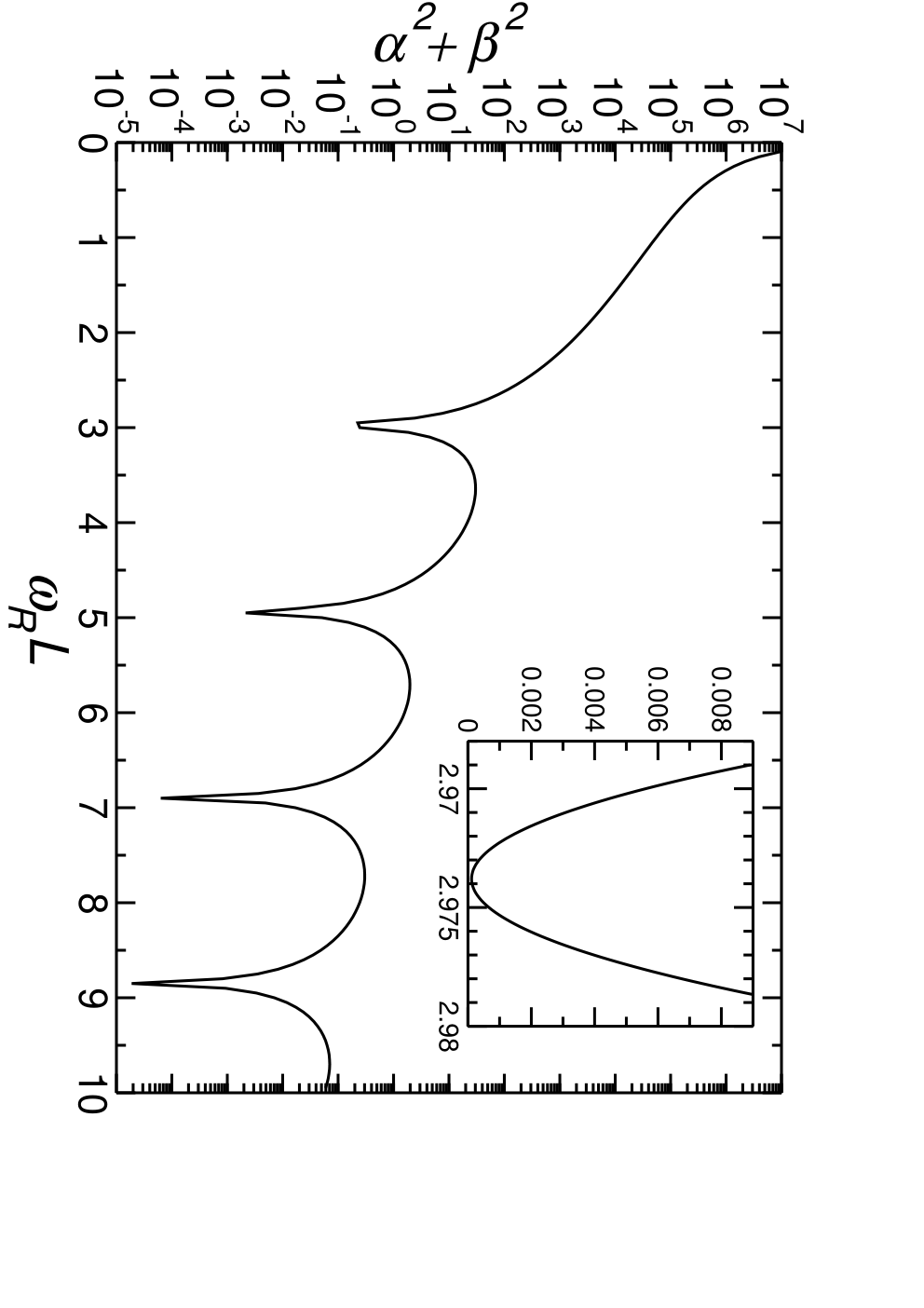 |
Fig. 2 shows a typical plot of as a function of . The pronounced dips correspond to the location of a resonance, , and the inset shows a zoomed-in view of one such particular resonance. Once a minimum in is located, the imaginary part can be found by a parabolic fit of to the Breit-Wigner expression (1). Alternative (but equivalent) expressions are , where a prime stands for the derivative with respect to , evaluated at the minimum [1, 2]. We used these three different expressions to estimate numerical errors in the computed quasinormal frequencies. In the next subsections we briefly report on our results for and , respectively.
II.1 Scalar field perturbations
The series solution method presented by Horowitz and Hubeny [3] was used by Konoplya in Ref. [16] to compute quasinormal frequencies of small SAdS BHs. The series has very poor convergence properties for , and QNM calculations in this regime take considerable computational time. As seen in Fig. 1, the potential for small SAdS BHs is able to sustain quasi-bound states, so we expect the resonance method to be well adapted to the study of small BHs.
| series | resonance | |||
|---|---|---|---|---|
| 12 | 3.064 | 9.533 | 2.992 | 9.662 |
| 20 | 2.922 | 7.720 | 2.912 | 7.840 |
| 30 | 2.805 | 6.660 | 2.802 | 6.714 |
| 50 | 2.700 | 5.952 | ||
| 100 | 2.610 | 5.471 | ||
| 200 | 2.580 | 5.266 | ||
| 500 | 2.560 | 5.158 | ||
| 1000 | 2.554 | 5.125 | ||
| 2000 | 2.550 | 5.109 | ||
| 5000 | 2.550 | 5.100 | ||
In Table 1 we list QNMs for scalar field perturbations and for different BH sizes, comparing (where possible) results from the resonance method with Konoplya’s series expansion calculation. A cubic fit of our data for yields , a quartic fit yields , and fits with higher order terms basically leave and unchanged with respect to the quartic fit. The numerical results are consistent with Horowitz and Hubeny’s prediction that , and they are in very good agreement with analytic predictions by Cardoso and Dias [17], who derived a general expression for the resonant frequencies of small BHs in AdS for regime. Setting in Eq. (33) of Ref. [17], their result is
| (9) |
where is a non-negative integer and
| (10) | |||
For one gets , in excellent agreement with the fits. For general Eq. (9) predicts an dependence, in agreement with our results for . Moreover we find excellent agreement with the proportionality coefficient predicted by Eq. (10). Higher overtones are also well described by Eqs. (9) and (10).
Our results show that the resonant frequency always approaches the pure AdS value in the small BH limit, generally confirming the analysis by Grain and Barrau [5]. However our numerics disagree with Grain and Barrau’s semi-classical calculation of the monopole mode (). We find that all modes including the monopole reduce to pure AdS in the small BH limit. More precisely, as we find
| (11) |
with for , respectively.
 |
Our results for scalar field perturbations are visually summarized in Fig. 3, where we combine results from the resonance method and from the series solution (compare e.g. Fig. 1 of Ref. [18]). Modes with different coalesce in the large BH regime (top-right in the plot), as long as . As shown in Fig. 1, the potential for small SAdS BHs develops a well capable of sustaining quasi-stationary, long-lived modes. It should not be surprising that small and large BH QNMs have such a qualitatively different behavior.
II.2 Gravitational perturbations
We have also searched for the modes of Regge-Wheeler or vector-type gravitational perturbations. The potential (3) for gravitational perturbations of small BHs does not develop a local minimum. Nevertheless it develops a local maximum which, when imposing Dirichlet boundary conditions [see the discussion following Eq. (5)] can sustain quasi-bound states. For this reason we expect the resonance method to be useful also in this case.
For small BHs our numerical results agree with the following analytic estimate, derived under the assumption that [19]:
| (12) |
with
| (13) |
For and this implies , while a fit of the numerics yields . Again, approaches the pure AdS value in the limit :
| (14) |
For the fundamental mode we find .
III Long-lived modes in the eikonal limit
A recent study of the eikonal limit () of SAdS BHs suggests that very long-lived modes should exist in this regime [6]. Define to be the two real zeros (turning points) of . Then the real part of a class of long-lived modes in four spacetime dimensions is given by the WKB condition
| (15) |
where . Their imaginary part is given by
| (16) |
The prefactor , not shown in Ref. [6], can be obtained by standard methods [20, 21] with the result
| (17) | |||||
| WKB | resonance | |||
|---|---|---|---|---|
| 3,0 | 5.8668 | -16.40 | 5.8734 | -17.03 |
| 3,1 | 7.6727 | -12.61 | 7.6776 | -12.97 |
| 3,2 | 9.4189 | -9.40 | 9.4219 | -9.60 |
| 4,0 | 6.8830 | -22.13 | 6.8889 | -22.84 |
| 4,1 | 8.7139 | -18.30 | 8.7184 | -18.41 |
| 4,2 | 10.4960 | -14.65 | 10.4996 | -14.72 |
| 5,0 | 7.8945 | -28.64 | 7.8997 | -28.76 |
| 5,1 | 9.7426 | -23.97 | 9.7466 | -24.02 |
| 5,2 | 11.5482 | -20.03 | 11.5516 | -20.06 |
The resonance method is well suited to analyze the eikonal limit, especially for small BHs (for large BHs the existence of a dip in the potential well requires very large values of , which are numerically hard to deal with). In Table 2 we compare the WKB results against numerical results from the resonance method. Unfortunately machine precision limitations do not allow us to extract extremely small imaginary parts. The agreement with the WKB condition of Ref. [6] is remarkable, even for relatively small values of . Our numerics conclusively confirm the existence of very long-lived modes in the SAdS geometry, but the numerical results for the damping timescales disagree by orders of magnitude with the corresponding results by Grain and Barrau [5]. A reanalysis of the assumptions implicit in their method would be useful to understand the cause of this disagreement.
IV Conclusions and outlook
The method described here provides a reliable and accurate alternative to the series solution method [3], to be used in regimes where the former has poor convergence properties. Together, the two methods allow an almost complete characterization of the spectrum of BHs in AdS backgrounds, encompassing both small and large BHs. As an application of the method, we have explicitly confirmed the existence of the weakly damped modes predicted by Refs. [5, 6].
Extensions of the resonance method to higher-dimensional [3] and charged geometries [18, 22] should be trivial. Our techniques may be useful to verify the existence of the highly-real modes predicted by Ref. [7]. Finally, it would be interesting to investigate whether the resonance method described here is of any use to investigate the eikonal limit of QNMs in asymptotically flat BH spacetimes.
Acknowledgements
We are indebted to Luis Lehner and Andrei Starinets for conversations that started this project. This work was partially funded by Fundação para a Ciência e Tecnologia (FCT) - Portugal through project PTDC/FIS/64175/2006. P.P. thanks the CENTRA/IST for hospitality and financial help and the Master and Back foundation programme of Regione Sardegna for a grant. V.C. acknowledges financial support from the Fulbright Scholar programme.
References
- [1] S. Chandrasekhar and V. Ferrari, Proc. Roy. Soc. Lond. A 434, 449 (1991).
- [2] S. Chandrasekhar and V. Ferrari, Proc. Roy. Soc. Lond. A 437, 133 (1992).
- [3] G. T. Horowitz and V. E. Hubeny, Phys. Rev. D 62, 024027 (2000) [arXiv:hep-th/9909056].
- [4] T. Harmark, J. Natario and R. Schiappa, arXiv:0708.0017 [hep-th].
- [5] J. Grain and A. Barrau, Nucl. Phys. B 742, 253 (2006) [arXiv:hep-th/0603042].
- [6] G. Festuccia and H. Liu, arXiv:0811.1033 [gr-qc].
- [7] R. G. Daghigh and M. D. Green, arXiv:0808.1596 [gr-qc].
- [8] N. Andersson and K. E. Thylwe, Class. Quant. Grav. 11, 2991 (1994).
- [9] N. Andersson, Class. Quant. Grav. 11, 3003 (1994).
- [10] Y. Decanini, A. Folacci and B. Jensen, Phys. Rev. D 67, 124017 (2003) [arXiv:gr-qc/0212093].
- [11] V. Cardoso and J. P. S. Lemos, Phys. Rev. D 64, 084017 (2001) [arXiv:gr-qc/0105103].
- [12] I. G. Moss and J. P. Norman, Class. Quant. Grav. 19, 2323 (2002) [arXiv:gr-qc/0201016].
- [13] G. Michalogiorgakis and S. S. Pufu, JHEP 0702, 023 (2007) [arXiv:hep-th/0612065].
- [14] I. Bakas, JHEP 0901, 003 (2009) [arXiv:0809.4852 [hep-th]].
- [15] J. V. Rocha, JHEP 0808, 075 (2008) [arXiv:0804.0055 [hep-th]].
- [16] R. A. Konoplya, Phys. Rev. D 66, 044009 (2002) [arXiv:hep-th/0205142].
- [17] V. Cardoso and O. J. C. Dias, Phys. Rev. D 70, 084011 (2004) [arXiv:hep-th/0405006].
- [18] E. Berti and K. D. Kokkotas, Phys. Rev. D 67, 064020 (2003) [arXiv:gr-qc/0301052].
- [19] V. Cardoso, O. J. C. Dias and S. Yoshida, Phys. Rev. D 74, 044008 (2006) [arXiv:hep-th/0607162].
- [20] G. Gamow, Z. Phys. 51, 204 (1928).
- [21] S. A. Gurvitz, Phys. Rev. A 38, 1747 (1988).
- [22] B. Wang, C. Y. Lin and C. Molina, Phys. Rev. D 70, 064025 (2004) [arXiv:hep-th/0407024].