Keywords: Cytoskeleton, Simulation, Flexible fibers, Langevin dynamics, Mechanics.
Collective Langevin Dynamics of Flexible Cytoskeletal Fibers
Abstract
We develop a numerical method to simulate mechanical objects in a viscous medium at a scale where inertia is negligible. Fibers, spheres and other voluminous objects are represented with points. Different types of connections are used to link the points together and in this way create composite mechanical structures. The motion of such structures in a Brownian environment is described by a first-order multivariate Langevin equation. We propose a computationally efficient method to integrate the equation, and illustrate the applicability of the method to cytoskeletal modeling with several examples.
1 Introduction
The internal architecture of living cells relies largely on microscopic fibers, which form the cytoskeleton with their associated proteins. These fibers have remarkable mechanical properties. Microtubules and actin filaments for instance have persistence lengths of 5 mm and 20 m, respectively, and can sustain pico-Newtons of force without breaking [1]. Yet these fibers can also be broken down quickly, because they are formed by the non-covalent assembly of protein monomers. Filament ends can grow or shrink, or even alternate between those two states in a remarkable process called dynamic instability [2, 3]. Structurally, the monomers in microtubules and actin filaments assemble head to tail in a regular manner. On the resulting polar lattices, mechano-enzymes called molecular motors (for example kinesin on microtubules or myosin on actin-filaments) use chemical energy to move directionally [1] or to organize the filaments in space [4]. Furthermore, specific enzymes control the filaments by regulating nucleation, assembly/disassembly or even by severing the filaments.
The cytoskeleton is involved in multiple cellular processes such as cytokinesis, motility, polarization and mitosis. These functions are accomplished by many filaments working together. In this way, a set of dynamic or short-lived filaments may form a stable larger assembly, as exemplified by the mitotic spindle [4]. Many of the enzymes involved in the assembly of these structures are part of multi-functional entities [5, 6, 7]. For example, motors form oligomers that can actively connect filaments together [4]; motors may be able to disassemble filaments [6]; nucleation can be controlled such that it occurs on existing filaments [8, 9]; crosslinkers may be polarity-specific [10] and motors are sometimes linked to proteins that track the tips of growing microtubules [7, 11, 12, 13]. Generally speaking, modularity allows the cytoskeleton to be reprogrammed, for example at different stages of the cell cycle. It allows cells to reuse the same functional elements to achieve different tasks and multiplies the number of way in which the organization of fibers can be regulated. This modularity is certainly a consequence of the combinatorial exploration operating during natural selection [14]. In any case, the cytoskeleton in addition to fibers contains a kit of activities which can be combined in many ways.
Biological systems are hard to understand, and theory is necessary to approach the non-intuitive aspects [15]. It is notable that many models in the cytoskeleton field often include the same basic elements (for a recent review on this subject, see [16]). This reflects the inherent modularity of the biological design illustrated briefly in the previous paragraph, and also affects the modeling approach. It implies that it is worthwhile to build a computer simulation to model a few basic elements, if these elements can be combined freely to rapidly model diverse situations. In practice, the elements of the simulation (eg. a model of kinesin, or a model of a severing enzyme) can even be implemented, tested and benchmarked by different teams of experts for each aspect of the system. Sharing computer code in this way can in fact be a practical mean to combine the efforts of the community.
Writing a cytoskeletal simulation is likely to be a collective task also because it is a demanding project, involving multiple aspects: (a) chemical reactions that occur inside cells, (b) transport along fibers, for example the motion of molecular motors, (c) assembly dynamics of cytoskeletal fibers and (d) motion and deformation of fibers. Fortunately, numerous algorithms are available for certain of these aspects, in particular for the reaction-diffusion (see [17, 18]). Transport along fibers can be modeled with advection equations, or with more details of the motion of the motors [19]. The assembly dynamics of fibers has been the subject of much research and cannot be reviewed here (see [16]). The deformation of the fibers is a classical mechanical problem (see for example [20, 21]). However, the scale of living cells is associated with many specific features. In particular, Brownian motion plays a fundamental role, inertia is negligible [22] and the fibers are dynamic: they can lengthen or shorten by self-assembly. As a consequence, the physics of biological fibers is fundamentally distinct from other mechanical systems. In brief, public or commercial codes are not adapted to simulate the cytoskeleton.
The purpose of this paper is to describe a method to calculate the mechanics of an ensemble of connected fibers and other objects, which is the basis of a cytoskeletal simulation such as cytosim. The physics of such system is described by a Langevin equation (for an introduction, see [23]) that recreates the Brownian motion of the fibers and includes bending elasticity, fiber-fiber interactions and external force-fields. Following earlier work [24, 25], we use constraints in order to maintain the length of the fibers. This is an alternative to methods in which potentials are used to represent the longitudinal stiffness of fibers. We extend this approach by introducing an implicit integration scheme. Our method was first used to simulate the effects of motor complexes on two radial arrays of microtubules (asters) [26], and more recently the assembly of anti-parallel microtubule arrays in S. pombe [7] and the positioning of the spindle in the C. elegans embryo [27]. A major aim of these simulations was to reconstitute the system’s operation in silico, from established physical principles. This offers two major advantages: i) the assumptions of the model are well defined and can always be modified; ii) any property of the system can be measured easily. This facilitates further investigations. For example we could systematically simplify the model in order to identify a minimal set of working properties [7]. In addition, we could identify the parameter range under which the system can operate [27]. However, for these results to be valid, the systems operation needs to be reproduced correctly at the first place! To maximize the chances of success, it is desirable to reconstitute the mechanics in a physically sensible and accurate way. One may otherwise derive conclusions which do not apply to the real system.
In this paper, we focus on the mechanical aspects of the fibers, and explore the numerical resolution of the associated equations. We first describe objects that in addition to fibers are useful for simulating different cellular skeletons. We then present the equation of motion and discuss its numerical integration. We examine the numerical stability of the resulting method and discuss how it affects the simulation speed. Finally, we discuss how other aspects of the cytoskeleton can be added to extend the mechanical calculation.
2 Objects
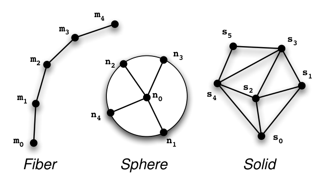
More accurate mechanics can be achieved if we introduce two new objects in addition to fibers: spherical sets of points (spheres) and non-deformable sets of points (solids). These objects are also described with points but have different morphologies (see fig. 1). The mechanical properties are also distinct. While fibers may bend, the solids do not deform. The spheres can represent spherical viscous membranes such as vesicles. Any number of objects can be combined in various ways to build complex cytoskeletons. For example, to simulate interacting microtubule asters [26], fibers were positioned around a solid using static links (see fig. 2A). The solid represented in this case the organelle (called the centrosome) which in the cell generates microtubules in a radial fashion. In vivo as well as in the simulation, the resulting structure is radially symmetric, and the fibers have their ends mechanically joined together. Two such asters were further connected by another solid, to model the positioning of the mitotic spindle in C. elegans [27]. In this case, the additional solid represented the pole-to-pole mechanical connection achieved by the mitotic spindle. To simulate nuclear positioning in S. pombe, fibers (microtubules) were attached to a sphere, and the ensemble was confined in a cylindrical volume (see fig. 2B). The fibers and the sphere represented microtubules and the cell nucleus, which are attached also in the real cell. To model the formation of anti-parallel microtubule arrays in S. pombe [7], fibers where connected by motors and other crosslinkers (see fig. 2C). Using fibers and solids, it is also possible to model the segregation of parM plasmids in E. coli (see fig. 2D), a process which depends on actin-like filaments [28]. The objects can naturally be combined in many more ways than illustrated here. This enables diverse cellular mechanics to be reproduced, and consequently widens the application scope of the method. This freedom is intimately linked to the structure of the master equation that will be examined below, and to the way it is integrated numerically.
3 Constrained Langevin Dynamics
In the simulation, fibers and other objects are described by points. The coordinates of the points are collected in a vector of size , for a system of points in dimension . Following Langevin (for a simple introduction, see [23]) the equation of motion reads:
| (1) |
of size contains the forces acting on the points at time . It includes object-specific forces such as bending elasticity, and all the links between different objects. of size summarizes the random molecular collisions leading to Brownian motions; it is a stochastic non-differentiable function of time. The matrix contains the mobility coefficients of the object-points, which will be defined later for each object.
In addition, certain distances between points inside the objects () must be conserved during the motion. To satisfy these constraints, we perform a step of the dynamics in a subspace tangent to the manifold defined by the constraints, and project the result on the manifold. The procedure can be explained simply for a point constrained to move at a distance from a fixed position (see fig. 3). To calculate the motion of , we first write its dynamics in the plane tangent to the sphere at the current position (this is the plane allowed by the constraint ). The restricted dynamics is integrated implicitly, and the result projected on the sphere to restore the constraint exactly. This approach can be generalized as described next.
4 Numerical integration
From an initial configuration, the system is calculated by discrete time steps (see [29] for a general discussion on numerical integration). To calculate from , the equation (1) is integrated implicitly. We will discuss the advantages of using an implicit rather than an explicit integration in section 9, and concentrate here on the practical issues. For an implicit integration, we need to express linearly as , where the square matrix contains the stiffness coefficients associated with the interactions, and the vector contains the constant forces. This linearization is obtained by summing over all the interactions present at time (see fig. 6). In our simulations, many of the interactions were modeled as harmonic potentials for simplicity, and are therefore already linear. Non-linear interactions simply need to be linearized at this point. In particular, the linearization of the constraints leads to an orthogonal projection , which will be defined later for each object. To obtain a finite difference scheme for the interval , and are used at time , but is used at (using instead of is the basis of implicit integration):
leading to a system of linear equations:
| (2) |
where , , . The “simulated Brownian” is a vector , where are independent normally distributed numbers (derived from uniformly distributed pseudo-random numbers [29]). The factors represent the magnitude of the Brownian motion during a lapse of time . We will see later how they are obtained by calibrating the diffusive motion for the objects. The equation can be solved to obtain , since both the right-hand side and the matrix are known. It would be inefficient to invert the matrix, because the system is sparse (it only has few non-zero coefficients). This is true of matrix , as long as objects are only connected to few others. This is also true of which is block-diagonal: it has one block for each object on the diagonal, but the rest of the coefficients are null. This is because the constraints never involve points from different objects, and the projection can thus be done independently for each object. In this situation, it is advantageous to solve the linear system using an iterative method [29]. Different iterative solvers are adapted to different matrices. Because is non-symmetric, we have used the biconjugate gradient stabilized (http://www.netlib.org). This method iteratively converges toward the solution of the linear system, and can be stopped when the difference with the exact solution is below a certain threshold. We set this threshold to , with . In this way, the numerical error on remains below of the Brownian motion, and the approximate solution of (2) is practically indistinguishable from the real one. In practice, it is wise to systematically vary and for each application to check the convergence of the method. It is easy to verify, for example, that more stringent values of produce the same results.
Finally, since equation (2) is obtained by linearization, an additional correction is necessary to re-establish the constraints. The result of equation (2) is projected back on the manifold associated with the constraints [26]. This introduces corrections which are second-order in . In the following sections, we will call this procedure ‘reshaping’ the objects. We now survey how fibers, spheres and solids are represented in space, their mobility coefficients, projection operators and ‘reshaping’ procedure. The interactions between objects (which contribute to and ) will be described subsequently.
5 Linear set of points (fiber)
Fibers are modeled as infinitely thin linear objects behaving like elastic, non extensible rods [26]. Each fiber is represented by equidistant model-points , for , separated by a distance . A fiber is polar: is the minus-end and the plus-end. The number of segments is adjusted as a function of the total length of the fiber. Points are added or removed, in order to always minimize , for each fiber as it grows or shrinks (see fig. 4). The desired segment length is a parameter affecting the precision of the simulation. To set , one may run a representative case with various values (for microtubules, is usually appropriate).
It is often necessary to interpolate between the model-points, when for example calculating the position of a molecule attached to the fiber. If and are the model-points on each side of , we use . The interpolation coefficient is calculated from the known relative positions of the three points along the fiber: . The model-points are themselves updated using this interpolation procedure at every time-step if the length of the fiber has changed (see fig. 4).
5.1 Bending elasticity
Fibers can bend under external forces and resist these forces elastically. The standard formula for bending elasticity [20] can be applied to strings of points. For any set of three consecutive points , , we approximate it linearly as a triplet of forces . Each triplet corresponds to the torque generated between two consecutive segments (see fig. 5). Furthermore, we have , with , where is the bending modulus of the fiber, and the length of each segment. The result was verified by comparing the buckling threshold in the simulation with Euler’s formula . The procedure is appropriate if is such that the angles between consecutive segments remain small during the simulation (not shown). Physically, the forces are isotropic, i.e. they can be written as a reduced matrix of size (and not ), obtained by adding several times the matrix ( is the tensor product). The final result is simple because points are distributed regularly over the length of the fiber (see fig. 5).
5.2 Mobility
The motion of an object at low Reynolds number is characterized by a mobility. This is defined by factors which link speed and force (speed = mobility force). These factors depend on the size and shape of the object, and on the viscosity of the surrounding fluid. For instance a straight cylinder has two mobility factors, because it is twofold easier to move in the longitudinal direction than in a transverse direction. This anisotropy could not be implemented simply, because fibers in the simulation may bend and adopt arbitrary shapes. An exact calculation would require finding the hydrodynamic interactions between all the points in the system. This can be done in the future, but for simplicity, we have so far used the averaged mobility of a straight rod of length and diameter : [30]. The logarithmic term is an effective hydrodynamic correction on the scale , which is either the length of the fiber, or a hydrodynamic cut-off, whatever is smallest. We derive a single mobility factors for the points representing a fiber: .
5.3 Projector associated with the constraints
In this section, we calculate the projection derived from the constraint that the length of the fiber should remain constant during the resolution of equation (1). For each fiber, the coordinates of the model-points are stored in a vector of dimension (for , correspond to , and to , etc). The motions of these points are determined by external forces , and additionally by internal forces . The speeds resulting from should be compatible with the constraints for . To calculate from , we first define the Jacobian matrix . In 3D, it reads:
Because the mobility coefficients are the same for all the points (, see sec. 5.2), the speed of the points is . This motion maintains the constraints if . Therefore must be such that . Furthermore, internal forces should not contribute to global motion or rotation of the object. This imposes that their work should be null for any motion compatible with the constraints: for any such that . This implies that , where is a vector of size (the Lagrange multipliers). We derive , and since of size is non-singular, , and finally . This shows that the total force can be obtained linearly as , with . From this result, it is clear that is an orthogonal projection ( is symmetric and idempotent ). Notice that is banded symmetric, and therefore easy to invert, which means that can be computed fast. (which depends solely on ) is one block of the operator used in equation (2).
Fibers are ‘reshaped’ to restore the constraints exactly after the model-points have been moved. This is done sequentially for , by moving the points in the direction of and in the opposite direction, to restore while conserving the center of gravity of the fiber.
5.4 Brownian motion
To simulate Brownian motion, a term is attributed to each fiber coordinate (equation 2). This term is most simply calibrated by considering diffusion in the absence of bending or external forces (, ). If we first assume in equation (2), we get . To produce a pure diffusion with a coefficient , one needs:
This holds true if is normally distributed, of mean zero and variance . We can use , where is a random number generated for each time step, and , as mentioned in section 4. From Einstein’s relation, we set , where is the mobility, the Boltzmann constant, and the absolute temperature. For a fiber with points, we use random numbers, independent and all normally distributed of variance . Projecting these numbers with produces the appropriate diffusion for the fiber, as well as thermally-driven deformations. For example, the translation of the center of gravity depends on the sum of all the terms in corresponding to the fiber, leading to a diffusion (with and not ).
6 Spherical set of points (sphere)
To simulate the nucleus of S. pombe and attach microtubules on its surface (see fig. 2B), we implemented a ‘spherical set of points’ of radius . Such object is composed of a point in the center, and additional points on the periphery. If we define , the constraints are . A sphere moves as a rigid body, and the peripheral points behave as if they were embedded in a viscous surface (see fig. 1). If is the force applied at point , the motion of the set reads:
where is the total force on the sphere, is the total torque calculated from the center, and where
is the projection on the plane tangent to the sphere in . , and are the Brownian terms. Note that these equations would not describe a set of peripheral points articulated around a central node. For example, the motion of the center depends on the sum of all the forces applied to the object, and not only on the force applied in . This in fact corresponds to a sphere with points on its surface. To keep track of the orientation of the sphere, we also included three reference points on the surface, which form with a reference frame associated to the sphere. The motion of these reference points is entirely determined by the total torque on the sphere: , where as before . When the object needs to be ‘reshaped’, the peripheral points are simply projected on the surface ( is not moved).
6.1 Mobility and Brownian Motion
The equations involve three mobility factors: the translation and rotational mobility of the sphere and , and the mobility of the points in the surface . Stokes’ law can be used to set and , if the sphere is surrounded by a large volume of fluid. The mobility coefficients for the points in the surface can also be calculated [31]. As described above, points undergo three different types of motion, and a random number in equation (2) is associated with each of these motions. The parameters are calculated by considering diffusion in the absence of other forces ( and ). For the translational diffusion of the sphere, the result from equation (6) is obtained as previously for the fiber: . Rotational diffusion is calibrated using equation (6). If is fixed on the surface, we get . This should be a rotational diffusion of a point on a sphere:
Since , we can use for a random vector with independent components of mean zero and variance . A peripheral point also diffuses on the surface, which in equation (6) is described by . The projection of should diffuse in 2D:
Since is the identity in the tangent plane, we used for a vector with independent components of mean zero, and variance .
7 Non-deformable set of points (solid)
We also implemented non-deformable objects called solids (see fig. 1) in which the points move together in such a way that the shape and size of the set is conserved. The number of points in a solid, and their positions can be chosen arbitrarily, and each point is associated with a radius . The mobility of the solid is derived from Stokes’s result for the spheres of center and radius , neglecting for simplicity the hydrodynamic interactions between the spheres. It is possible to include points with provided that . In our previous work, we have actually used solids where only one was non-zero. These solids moved like isolated spheres, and the points where positions to which forces could be applied.
7.1 Mobility and Constrained Motion
Because the set of points should not deform, its elementary motion during a time-step can be written as , where and are instantaneous translation and rotation speeds. The spheres of radius in a medium with viscosity have a translational drag coefficient , and a rotational drag coefficient [30]. The forces and torques resulting from the friction of the fluid on the sphere thus read:
and should match the externally applied forces :
This set of four equations can be solved algebraically in both 2D and 3D, to express and as a function of the external forces . The result always fits in the format of equation (1). It is actually not necessary to calculate the matrix to run a simulation. It is more efficient to calculate and when the product is needed. To ‘reshape’ a solid, one may restore a reference configuration in the current position and orientation. For this, the best translation and rotation which brings the reference points onto the current points is calculated [32]. The current points are then replaced by the transformed reference configuration. The Brownian components are calibrated as described before.
8 Interactions between objects
The three objects defined previously can be linked together using elementary interactions. By adding the contributions of all these interactions in the system, we obtain the linearized force , which enters equation (2). In practice, each elementary interaction leads to a small matrix, which needs to be added to the matrix and vector , at the right rows and columns to correspond to the appropriate points (see example on figure 6). It is necessary to repeat the procedure at every time step, because the position of the interactions may change with respect to the model-points. We define four interactions in the case where they connect model-points of the objects. We later explain the procedure to connect intermediate positions between the model-points. This approach can be generalized to more complicated interactions if necessary. For example, it is possible to implement a ring able to slide along a fiber with viscous resistance [33].
8.1 Connecting an object to a fixed position.
The simplest way to immobilize an object is to attach a point within the object to a fixed position . If the stiffness of the link is , the resulting force is . In practice, this means adding at one diagonal position in matrix , and to the vector (see fig. 6). Such interactions are used to model gliding assays (see fig. 8) in which motors immobilized on a surface propel fibers in solution. Each attached molecular motor leads to an elementary interaction where corresponds to the place of immobilization, and corresponds to the position on the fiber at which the motor domain is attached.
8.2 Connecting two objects.
Points from two different objects can be connected by a link of stiffness . The forces between the points are . These elementary interactions are effective to model oligomeric motors [26] and more generally any entity able to connect two fibers together (see fig. 2C). In the case of an oligomeric motor, and are the positions to which the two motor domains are attached on the fibers.
8.3 Confinement in a convex shape.
To confine the objects inside a convex shape, we use a harmonic potential that is flat inside the allowed region, and rises quadratically away from its edge. Hence, a point outside the cell volume is subject to a force , where is the closest point to on the edge of the allowed volume. Because is also the orthogonal projection of , the force corresponds to a friction-less edge. We linearized as , where is a unit vector in the direction of . This linearization corresponds to the tangent plane in , and usually gives a good approximation of as long as the curvature is small. To confine a fiber, it is sufficient to follow the procedure for its model-points, if the volume is convex, which is the case for example of the cylindrical yeast S. pombe (see fig. 2B). To confine the nucleus of radius in the same volume, we used a cell volume reduced by . In this way only the center of the sphere needs to be tested.
8.4 Connecting two objects at a given distance.
A Hookean spring of stiffness with a non-zero resting length between two points and corresponds to:
with . This force should be linearized for , leading for to a term in and a contribution in which is:
| (6) |
and the opposite contributions for . This interaction can be useful to introduce a repulsion between the points. It can for example represent the physical interaction between the nuclear membrane and the microtubules in S. pombe (see fig. 2B).
8.5 Interpolation of forces
We have discussed connections which were attached to model-points. However, in the case of a fiber, a molecule may bind at any position , which is likely to be between two model-points and . When this happens, is interpolated from the flanking model-points using a coefficient in . In the same way, a force applied in can be distributed to the model-points as and . Since this procedure preserves any linearity in the relationship between force and coordinates, the different matrix elements mentioned previously can be used with interpolated points, provided they are multiplied left and right by an appropriate weight matrix. We can illustrate the procedure for the simplest connection of stiffness between two points and (section 8.2), which reads:
When and are model-points, this matrix is a reduction of , corresponding to the , or - subspaces. This is sufficient in this case because a Hookean spring of null resting length is isotropic, that is to say it does not mix , and coordinates, and applies similarly to each subspace. This is not the case for all interactions discussed in this section, and it is often necessary to calculate a full matrix. Moreover, when and are intermediate positions between the model points, we have two indices and two interpolation coefficients such that and . If we define and , and
we get:
The resulting matrix is , with . We derive that a matrix made by adding multiple such interactions is symmetric negative-semidefinite (, for any ). The fact that this is true for any configuration of the connections guarantees the numerical stability of the method, as explained next.
9 Numerical Stability and Performance
We have described all the components of equation (2) which describes the collective mechanics of cellular fibers and other objects. The necessary steps of the calculation are summarized in figure 7. It is useful at this stage to examine the method mathematically. This is usually done by looking at two properties: precision and numerical stability [29]. The precision is a measure of how the typical error behaves when the time-step becomes small. The numerical stability is a measure of how large can be, before the calculation fails. Numerical precision is important for deterministic equations, for example to predict the trajectories of celestial bodies. However, this is not so critical at the cellular scale. In fact, to simulate the Brownian motion present in the cell, a random term was included in equation (2). The presence of this ‘noise’ indicates that the physics itself limits the precision at which the position of an object can be predicted. This fact undermines the usefulness of high precision schemes. The implicit method that we have described is of order one: the step’s error scales like , which is better than the physical ‘noise’ in . We found that it was not practically useful to use higher order numerical schemes.
In contrast, the numerical stability of the method is most important. Indeed, explicit schemes usually converge only if the time-step is small. In general, a condition like must be fulfilled, where is the mobility of a point in the system, and the stiffness of the interaction potential. For example, we looked at a test-case in which a microtubule is pushed by immobilized motors (see [25] and Fig. 8). It can be simulated explicitly only if s, but the implicit method can use larger time-steps. To achieve this stability, we treated the repulsive and attractive interactions in the system differently. Compressive forces in the fibers (which are repulsive in nature) were replaced by constraints. All the other forces were attractive. This ensured that would be negative-semidefinite (this result was proven in section 8.2 for Hookean interactions of null resting length). Mathematically, because is an orthogonal projection, we can show that the eigenvalues of are always greater than , for any value of . This implies that our integration scheme is unconditionally stable. For the other elementary interactions, some instabilities may appear, but only for very high values of the time step (not shown).
Beyond stability, other considerations naturally limit the choice of . In particular the iterative solver might not converge when is large. The optimal time-step generally depends on the problem studied, and it is best to perform systematic trials to find it. For the test-case (see fig. 8), the results are consistent for ms. This means that a value of or ms would be appropriate. The computational requirements depend on the total number of steps (total time/time-step), but also on the cost of individual steps. An implicit step of integration is always more costly than an explicit step, because a linear system must be solved. However, the use of sparse matrix techniques reduces the additional work. In practice the considerable reduction in the number of steps makes implicit simulations faster (in the test-case, this gain is , using ms instead of s). Increasing the execution speed is essential if many simulations need to be performed. Implicit methods require increased numerical labor, of which we have illustrated the main difficulties. Using the method described here, we can simulate the examples shown in figure 2 B, C & D much faster than real time using one processor (www.cytosim.org).
10 Other Elements of a Cytoskeletal Simulation
In addition to mechanics, a cytoskeletal simulation such as cytosim must include additional aspects such as the motion of molecular motors, their binding/unbinding dynamics, as well as the transitions between growth and shrinkage of dynamic fibers. These processes can be modeled most simply by executing small sub-routines after the Brownian mechanics has been calculated, because they correspond to independent operations (see fig. 7). However, two particularly important aspects of cytoskeletal physics need to be mentioned. Firstly, only in very particular cases can we approximate the system as a well-mixed reactor. At least some of the molecules should be spatially resolved. Secondly, the mechanics commonly affects the chemistry. For instance the rates of certain key reactions are force-dependent. This is the case for the unbinding rates of molecular motors and for their stepping rate (see below). Because these elements are essential for modeling the system accurately, it will rarely be possible to apply algorithms developed for purely chemical systems (eg. the Gillespie algorithms [34] or even spatially resolved methods [35]) without extensive modifications. We can however use simple and robust simulation strategies, as illustrated below in the case of molecular motors.
10.1 Modeling Molecular Motors
In cytosim, a motor is characterized by a position, when it is not attached, and by a pointer to a fiber and a curvilinear abscissa, when it is attached (see fig. 9). The abscissa is the distance, measured along the fiber, between a reference and the attachment position. It is necessary to use a reference which is fixed with respect to the physical lattice, because the model-points of a fiber are themselves updated as the fiber grows (see fig. 4). This description neatly separates the details of how the mechanics is implemented from the routines simulating the motors per se. This means that the interface with the rest of the program can be very simple, with only two procedures: step(f) and attach(m).
10.1.1 Active Motion.
The first procedure step(f) simulates the possible actions of a bound motor. The argument is the load of the motor calculated during the collective mechanics. The procedure should decide to detach the motor, or to update the abscissa according to a microscopic model for the interval . For a well characterized motor like kinesin, a classical model is based on the measured characteristics of the motion: the abscissa is increased by . In addition, a force-dependent unbinding rate is used to model the dissociation from the fiber. , , and are characteristics of the motor that have been measured for kinesin [1]. With this model, the fibers are continuous tracks along which motors may be located anywhere. Alternatively, we may model the motion of a motor as a succession of discrete stochastic steps. In this case, the motor does one of four things: stay immobile, detach, take a step toward the minus-end or take a step toward the plus-end. This means that if the motor does not detach, the abscissa is either unchanged, or it is increased or decreased by the step size (8 nm). The procedure step(f) calculates the probabilities of these events as a function of the force for the interval , and selects one of them. This model is quite attractive, because these probabilities are actually available for kinesin [36]. Most models describing the movement of motors [19] can be summarized similarly with a function step(f).
10.1.2 Attachment to Fibers.
The second procedure necessary to model motors, attach(m) simply decides if a unbound motor binds or not to a site . Usually the model would specify , a maximum distance at which a motor may bind from its current position (see fig. 9). In addition, the molecule would bind at the closest site on the fiber (the orthogonal projection) with a certain molecular binding rate (). To simulate attachments, one therefore needs to first find the fiber-segments which are closer than , typically from all the positions at which molecular motors are located. For each point , the list of candidates should then be shuffled, to ensure a random ordering of the segments. The molecular binding rate can finally be tested sequentially for each segment in the list, for example by comparing with a random number in [0,1]. The first successful trial is followed by attachment. If done naively, the first step of the operation may require calculating the distance of all points to all fiber-segments, and thus a great deal of computation for many motors. To avoid this bottleneck in cytosim, a divide and conquer algorithm was developed (see fig. 10). Its goal is to limit the number of segments that need to be tested to find those which are close to . The geometrical distance between and these segments is calculated using the vector cross-product to exactly determine which ones are closer than . Reducing the number of tested segments is sufficient to accelerate the simulation.
11 Conclusion
The method described here is efficient to simulate sparsely connected networks of filaments. It applies to many in vivo situations, because the connections between fibers are usually mediated by proteins that are small compared to the fibers, and consequently the fibers are only locally connected. We have modeled fibers as oriented lines, which is sufficient to calculate the extent of bending. It may be necessary in the future to include more details such as writhe, since cytoskeletal fibers also have a torsional rigidity. The method can be extended in several other ways. One could for instance easily model discrete binding sites on the fibers. This may be important if the fibers are highly covered and molecules compete or interact while bound to the lattice. It is also possible to extend the overdamped mechanics by adding hydrodynamic effects. It will be very exciting to integrate fiber mechanics with membrane dynamics, since membranes and cytoskeleton contribute synergistically to cellular architecture, but this might take some time. Cellular chemistry, reaction-diffusion of the components in the cell, gene expression networks, can be added more simply. This can be done by interfacing our software with other tools (eg. the Virtual Cell project), which already cover some of these aspects of physiology. We did not discuss here implementation issues, but the scale of the task should remind us of their importance. Software modularity is essential to divide the development effort in separate projects of manageable size. Sub-models or algorithms should be developed and tested separately, in such a way that they can be added or removed from the integrative software easily. Dividing the work among different groups is the best way to produce the high-quality cellular simulations that biology needs.


References
- [1] Jonathon Howard. Mechanics of Motor Proteins and the Cytoskeleton. Sinauer Associates Incorporated, 2001.
- [2] A Desai and T Mitchison. Microtubule polymerization dynamics. Annu Rev Cell Dev Biol, 13:83–117, 1997.
- [3] Ethan Garner, Christopher Campbell, and R Mullins. Dynamic instability in a dna-segregating prokaryotic actin homolog. Science, 306(5698):1021–5, Nov 2004.
- [4] T Wittmann, A Hyman, and A Desai. The spindle: a dynamic assembly of microtubules and motors. Nat Cell Biol, 3(1):E28–E34, Jan 2001.
- [5] Christine Blaineau, Magali Tessier, Pascal Dubessay, Lena Tasse, Lucien Crobu, Michel Pagès, and Patrick Bastien. A novel microtubule-depolymerizing kinesin involved in length control of a eukaryotic flagellum. Curr Biol, 17(9):778–82, May 2007.
- [6] Vladimir Varga, Jonne Helenius, Kozo Tanaka, Anthony Hyman, Tomoyuki Tanaka, and Jonathon Howard. Yeast kinesin-8 depolymerizes microtubules in a length-dependent manner. Nat Cell Biol, 8(9):957–962, Sep 2006.
- [7] Marcel Janson, Rose Loughlin, Isabelle Loïodice, Chuanhai Fu, Damian Brunner, François Nedelec, and Phong Tran. Crosslinkers and motors organize dynamic microtubules to form stable bipolar arrays in fission yeast. Cell, 128(2):357–68, Jan 2007.
- [8] Marcel Janson, Thanuja Setty, Anne Paoletti, and P Tran. Efficient formation of bipolar microtubule bundles requires microtubule-bound gamma-tubulin complexes. J Cell Biol, 169(2):297–308, Apr 2005.
- [9] Nicole Mahoney, Gohta Goshima, Adam Douglass, and Ronald Vale. Making microtubules and mitotic spindles in cells without functional centrosomes. Curr Biol, 16(6):564–569, Mar 2006.
- [10] Isabelle Loïodice, Jayme Staub, Thanuja Setty, Nam-Phuong Nguyen, Anne Paoletti, and P Tran. Ase1p organizes antiparallel microtubule arrays during interphase and mitosis in fission yeast. Mol Biol Cell, 16(4):1756–1768, Apr 2005.
- [11] J Christian Ambrose, Wuxing Li, Adam Marcus, Hong Ma, and Richard Cyr. A minus-end-directed kinesin with plus-end tracking protein activity is involved in spindle morphogenesis. Mol Biol Cell, 16(4):1584–92, Apr 2005.
- [12] Gohta Goshima, François Nedelec, and Ronald Vale. Mechanisms for focusing mitotic spindle poles by minus end-directed motor proteins. J Cell Biol, 171(2):229–40, Oct 2005.
- [13] E E Morrison. Action and interactions at microtubule ends. Cell Mol Life Sci, 64(3):307–17, Feb 2007.
- [14] John Gerhart and Marc Kirschner. Cells, Embryos, and Evolution. Blackwell Science, 1997.
- [15] Alex Mogilner, Roy Wollman, Gul Civelekoglu-Scholey, and Jonathan Scholey. Modeling mitosis. Trends Cell Biol, 16(2):88–96, Feb 2006.
- [16] Eric Karsenti, Francois Nedelec, and Thomas Surrey. Modelling microtubule patterns. Nat Cell Biol, 8(11):1204–1211, Nov 2006.
- [17] Caroline Lemerle, Barbara Di Ventura, and Luis Serrano. Space as the final frontier in stochastic simulations of biological systems. FEBS Lett, 579(8):1789–94, Mar 2005.
- [18] Maciej Dobrzynski, Jordi Vidal Rodríguez, Jaap A Kaandorp, and Joke G Blom. Computational methods for diffusion-influenced biochemical reactions. Bioinformatics, 23(15):1969–77, Aug 2007.
- [19] Anatoly B Kolomeisky and Michael E Fisher. Molecular motors: a theorist’s perspective. Annual review of physical chemistry, 58:675–95, Jan 2007.
- [20] Lev Landau and E Lifshitz. Theory of Elasticity. Butterworth Heinemann, 1986.
- [21] Robert Leighton Richard Feynman and Matthew Sands. The Feynman Lectures on Physics. Addison-Wesley, 1989.
- [22] E Purcell. Life at low reynolds number. Am J Phys, 45(1):3–11, 1977.
- [23] Don S. Lemons. An Introduction to Stochastic Processes in Physics. The Johns Hopkins University Press, 1949.
- [24] J Deutsch. Theoretical studies of dna during gel electrophoresis. Science, 240(4854):922–924, May 1988.
- [25] Bourdieu, Duke, Elowitz, Winkelmann, Leibler, and Libchaber. Spiral defects in motility assays: A measure of motor protein force. Physical Review Letters, 75(1):176–179, Jul 1995.
- [26] Francois Nedelec. Computer simulations reveal motor properties generating stable antiparallel microtubule interactions. J Cell Biol, 158(6):1005–1015, Sep 2002.
- [27] Cleopatra Kozlowski, Martin Srayko, and François Nedelec. Cortical microtubule contacts position the spindle in c. elegans embryos. Cell, 129(3):499–510, May 2007.
- [28] Jakob Møller-Jensen, Jonas Borch, Mette Dam, Rasmus Jensen, Peter Roepstorff, and Kenn Gerdes. Bacterial mitosis: Parm of plasmid r1 moves plasmid dna by an actin-like insertional polymerization mechanism. Mol Cell, 12(6):1477–1487, Dec 2003.
- [29] William Press, Saul Teukolsky, William Vetterling, and Brian Flannery. Numerical Recipes, Second Edition. Cambridge University Press, 2002.
- [30] Howard Berg. Random walk in Biology. Princeton University Press, 1993.
- [31] P Saffman and M Delbrück. Brownian motion in biological membranes. Proc Natl Acad Sci U S A, 72(8):3111–3113, Aug 1975.
- [32] Berthold Horn. Closed-form solution of absolute orientation using unit quaternions. Journal of the Optical Society of America A, 4:629, 1987.
- [33] Stefan Westermann, Hong-Wei Wang, Agustin Avila-Sakar, David Drubin, Eva Nogales, and Georjana Barnes. The dam1 kinetochore ring complex moves processively on depolymerizing microtubule ends. Nature, 440(7083):565–9, Mar 2006.
- [34] Daniel T Gillespie. Stochastic simulation of chemical kinetics. Annual review of physical chemistry, 58:35–55, Jan 2007.
- [35] Johan Hattne, David Fange, and Johan Elf. Stochastic reaction-diffusion simulation with mesord. Bioinformatics, 21(12):2923–4, Jun 2005.
- [36] N J Carter and R A Cross. Mechanics of the kinesin step. Nature, 435(7040):308–12, May 2005.