Current-driven and field-driven domain walls at nonzero temperature
Abstract
We present a model for the dynamics of current- and field-driven domain-wall lines at nonzero temperature. We compute thermally-averaged drift velocities from the Fokker-Planck equation that describes the nonzero-temperature dynamics of the domain wall. As special limits of this general description, we describe rigid domain walls as well as vortex domain walls. In these limits, we determine also depinning times of the domain wall from an extrinsic pinning potential. We compare our theory with previous theoretical and experimental work.
pacs
72.25.Pn, 72.15.Gd, 72.70.+mI Introduction
Current-driven domain wall motion was first predicted and observed by Berger in the eighties.[1, 2] It was not until the discovery, in the nineties, of the spin transfer torque mechanism,[4, 3] that research on current-driven domain walls took off. Spin transfer torques on a domain wall can be understood on an intuitive level: the electrons which constitute the current have spin, and this spin rotates when it passes through the domain wall, as it aligns with the domain wall magnetization. By conservation of spin, there is an opposite torque on the magnetization of the domain wall, which leads to a net displacement of the domain wall in the same direction as the electric current. Later, to explain some discrepancies with experiments, a so-called dissipative spin transfer torque (sometimes referred to as the non-adiabatic spin transfer torque) was added to the model.[5, 6] The value of the dimensionless parameter , which gives the strength of this torque, has been the subject of much debate. By now it is generally accepted that is of the same order as , the Gilbert damping parameter, but not necessarily equal to it.[9, 10, 11, 8, 7] Furthermore, neither nor needs to be constant. They depend on the properties of the material and are most likely also temperature dependent.
Several properties of current-driven domain walls have been studied. One particular subject of interest is the velocity of the domain wall. The effect of an external pinning potential and the depinning behavior, both without and with thermal fluctuations, were investigated experimentally.[13, 12, 14] There is also interest in more complex, higher dimensional domain wall models, like vortex walls.[17, 16, 15] These are especially attractive from an experimental point of view since their dynamics, such as precession in a potential and transformations between vortex walls and transverse walls, can be directly observed.[20, 18, 7, 19]
With a few exceptions,[21, 22, 25, 24, 23] most theoretical papers are restricted to the zero-temperature case. This is unfortunate, since experiments on current-driven domain walls are usually done at room temperature, and the relatively large current will heat up the sample even further. Furthermore, especially in the presence of a pinning potential, thermal fluctuations are anything but negligible. Domain pinning can be necessary, for instance to precisely locate a domain wall, but thermal depinning can also be useful to lower the critical current. This means that it is very important to understand the influence of thermal fluctuations on the behavior of the domain wall precisely and thoroughly. Here, we present a unified picture of previous work on domain wall motion at nonzero temperature that involved two of us, as well as new results following from this unified picture.
We start this paper with the Landau-Lifschitz-Gilbert equation, including both the reactive and the dissipative spin transfer torques. In Section II, we apply a variational principle to derive the general equations of motion for a domain-wall line including thermal fluctuations. In Section III we investigate the velocity of current-driven and field-driven rigid domain walls at nonzero temperature, while in Section IV we look at vortex domain walls in more detail. Both the rigid and the vortex domain wall are special cases of the general description given in Section II. In both sections, we start with the zero-temperature case, and then investigate the influence of thermal fluctuations. Pinning potentials are included in both models, and we examine thermal depinning. Each section is divided into three subsections: one in which the model is described, one in which we present our results, and a final one to make a comparison with other work.
II Domain-wall lines
In this section, we derive the equations of motion for a domain-wall line in a more detailed way than in previous work[21] and present new results obtained from this model. We derive the Fokker-Planck equation of the system, and determine the stochastic behavior under the influence of temperature. The model is then considered in the absence of extrinsic pinning so that there is only intrinsic pinning due to magnetic anisotropy. We determine the drift velocity of the domain wall as a function of the current through the system. Finally, we compare our model with other theoretical and experimental work available in the literature.
II.1 Model
Magnetization dynamics including spin-transfer torques are described by the Landau-Lifschitz-Gilbert equation [3, 4]
| (1) |
where is a unit vector in the direction of the magnetization. In this expression, the first term on the r.h.s. contains a contribution due to the effective field, which is written as the functional derivative of the micromagnetic energy functional of the system and an external magnetic field . For clarity, we denote positions in three-dimensional space with an arrow, and the directions of the magnetization by bold symbols. The second term describes Gilbert damping, which is characterized by the dimensionless parameter . The term proportional to on the l.h.s. is the reactive spin-transfer torque. The term proportional to on the r.h.s. corresponds to the dissipative spin-transfer torque and is characterized by the dimensionless parameter . The velocity is given by , where is the lattice constant, is the charge current and is its spin polarization. To facilitate a variational approach, we note that the Landau-Lifschitz-Gilbert equation is obtained from
| (2) |
where is a dissipation functional, and where denotes the action of the system. The dot is a time derivative . The action for the magnetization dynamics in the absence of current and field is given by
| (3) |
In this expression, is the spin stiffness, and are the hard- and easy-axis anisotropy, respectively. The function is the vector potential of a magnetic monopole which obeys and is required to reproduce the precessional motion of around the effective field.
The external field and the reactive spin-transfer torque are determined from the action . We take the external magnetic field to be spatially homogeneous and time independent . The action is given by
| (4) |
with a positive constant. The dissipation functional that describes the dissipative spin-transfer torque and the Gilbert damping is written as
| (5) |
As the last ingredient, we take into account thermal fluctuations. We add to the effective field in Eq. (1) stochastic contributions such that , where has white-noise correlations
| (6) | ||||
| (7) |
and where the indices label Cartesian coordinates. The strength is given by the fluctuation-dissipation theorem , which assures that, in the absence of field and current, the Boltzmann equilibrium distribution
| (8) |
is reached after sufficiently long times. In principle, Eqs. (2–6) describe the full magnetization dynamics. Obtaining results on finite-temperature average drift velocities of domain walls is however very cumbersome, especially in the presence of extrinsic pinning. We therefore use a variational method.
We obtain the specific form of our variational ansatz by varying the action in Eq. (3) for a time-independent magnetization. Using we find ,[26] where the primes denote derivatives with respect to . This equation has domain-wall solutions and , where is the domain-wall width and is the position of the domain wall.
The variational ansatz we use is and . A domain wall is now described by two collective coordinates and that represent the position of the domain wall line and the chirality at this position, respectively. Note that is the coordinate along the line, and also that there are other possibilities for the exact form of the ansatz, such as choosing a different domain-wall charge.
We choose the magnetic field pointing in the positive direction , . Furthermore, the current is taken in the positive direction. We find that the action in terms of the collective coordinates and is then given by
| (9) |
where is the number of magnetic moments in a domain wall, with the length of the sample in the and direction, respectively. We now substitute the ansatz in Eq. (5) to obtain the dissipation functional as a function of the collective coordinates
| (10) |
Upon variation of the total action in Eq. (9) with respect to and , and setting this equal to the variation of the dissipation function in Eq. (10) with respect to and , respectively, we obtain equations of motion for the collective coordinates
| (11) | ||||
| (12) |
We now add thermal fluctuations that contribute as stochastic terms to Eqs. (11) and (12), so that we obtain Langevin equations
| (13) | ||||
| (14) |
Here we take functional derivatives of an effective potential that is a functional of and . Allowing for an arbitrary potential due to disorder and inhomogeneities, this effective potential is given by
| (15) |
and also includes contributions from the micromagnetic energy functional, the external field, and spin-transfer torques. Note that in the absence of current, field and disorder, the potential in Eq. (15) is exactly the total micromagnetic energy .
The noise in Eqs. (13) and (14) obeys and , where . The strength can be determined from the Fokker-Planck equation, which for the Langevin equations (13) and (14) is given by[27]
| (16) |
By demanding that the equilibrium Boltzmann distribution function that follows from Eq. (8), given by
| (17) |
is a time-independent solution of the above Fokker-Planck equation, we find the strength of the thermal fluctuations as
| (18) |
We see that the noise obeys the fluctuation-dissipation theorem with an effective temperature . The temperature is therefore effectively reduced by the magnetic-moment density in the domain wall line.
II.2 Results
Two of us analyzed the model in Eqs. (13) and (14) in the presence of extrinsic pinning.[21] In this section, we focus instead on the clean situation, in which everywhere. In the case, the domain wall line will stay straight because the force on each point is exactly the same. Specializing to , we find that there is a critical current . Below this critical current, the domain wall will not be able to acquire a finite drift velocity. This phenomenon is usually called intrinsic pinning,[26] and it does not occur for . Above the critical current, the domain wall will acquire an average drift velocity, given by
| (19) |
In the presence of thermal fluctuations we can no longer assume that the domain wall remains straight, and we need to go through a rather more elaborate procedure to find the average drift velocity. More specifically, if there are thermal fluctuations, we can differentiate between the flow regime above , for which Eq. (19) still approximately applies, and the thermal regime below , in which the speed is finite, but goes with a different power law.
To find the behavior in the thermally assisted regime, we start by rewriting the Langevin equations to find just one equation for . We then specialize to the case without an external magnetic field, with , and take . We assume that because there is no potential that couples to and find
| (20) |
which describes the motion of a string in a tilted washboard potential, a problem that was investigated before in a different context by Büttiker and Landauer.[28] For , the string propagates by thermal activation. This occurs due to the formation of a nucleus, or of a kink-antikink pair in the string. That is, part of the string is moved over the potential barrier due to thermal activation. If this nucleus is large enough, the kink and antikink will proceed to move apart from one another, and the string propagates to the next potential valley. Two factors are important: the energy barrier that needs to be overcome to generate a sufficiently large nucleus, and the propagation velocity of the kinks (and antikinks).
Let us start with the former. It is given by , where is a time-independent solution of the differential equation , and represents a stationary configuration, corresponding to the motion from a local maximum and back. In the above, is given in units of . The result is shown in Fig. 1.

In the limit that we are close to the critical current, i.e. that , we can solve for exactly and find[28]
| (21) |
This formula indeed fits very well to the tail of our numerical curve. Note that the energy barrier remains finite as . The difference between the above formula and the numerical solution is at most 25%, suggesting we may use Eq. (21) to estimate the qualitative behavior of domain wall motion even at lower values of . In the limit that we have that . This limit is not shown in Fig. 1 as it applies only for very close to zero.
The other important quantity is the velocity at which the kink and antikink move away from one another. This velocity is found numerically by solving the equation
| (22) |
with , and finding the for which the solution which starts out at will go away from that point, and return to at . The universal curve for this velocity is shown in Fig 2.

The probability of creating sufficiently large nuclei follows an Arrhenius law . We now have all the necessary ingredients to find the average velocity of the string, which is proportional to . In the limiting case where the current is close to the critical one, we have that[28]
| (23) |
where is a function of as in Fig. 2. In Fig. 3, we have plotted this velocity for different temperatures.

II.3 Experimental Status
In many experiments, the nanostrip is sufficiently narrow that we can neglect deformations of the domain wall line and approximate it as being rigid, an approximation we treat in the next section. However, Yamanouchi et al.[29] have observed in their experiments with magnetic semiconductors that the domain wall looks wedge-shaped in the current-induced case, suggesting that deformations play a role in wide enough nanostrips.
Yamanouchi et al. also found that the velocity of the domain wall obeys a scaling law. More specifically, they fitted their data with a creep-like scaling law with an exponent . Recent experiments with ferromagnetic metals[30] have found the exponent which would imply[21] that the dissipative spin-transfer torque dominates in the creep regime in this case.
III Rigid domain walls
In this section, we simplify the model of domain-wall lines by assuming that the domain-wall coordinates are constant along the direction, the domain wall is then rigid. This simplification allows us to obtain various results analytically.
III.1 Model
As mentioned before, rigid domain walls obey , i.e., they are rigid in the direction. We expect this approximation to hold in the limit when is comparable to . We integrate Eqs. (13) and (14) over (which is quite trivial since there are no dependences anymore) to obtain the Langevin equations for a rigid domain wall (We use and equivalently for )
| (24) | ||||
| (25) |
We integrate the total potential in Eq. (15) to find (note that )
| (26) |
The stochastic correlations are found from
| (27) |
In our model, rigid domain-walls obey the fluctuation-dissipation theorem with effective temperature , i.e., the temperature is effectively reduced by the number of magnetic moments in the domain wall.
III.2 Results
III.2.1 Clean system, intrinsic pinning
We first focus on the case that the extrinsic pinning is zero. Substitution of from Eq. (24) into Eq. (25) then provides us with an equation that is independent of . Using the equilibrium solution of Eq. (16), we find the average velocity of the chirality . With this result and Eq. (24), we compute average drift velocities
| (28) |
where the average chirality velocity is given by[27] (we omit a factor )
| (29) |
In this expression, the dimensionless effective potential is given by
| (30) |
and the dimensionless effective field is defined as . The expressions in Eqs. (28) and (29) generalize the results by Duine et al.,[22] to include external magnetic fields and .
In the field-driven case, we set to find the behavior in Fig. 4. In the calculations, we use a fixed value for the damping parameter and several values for the temperature.

At zero temperature, the drift velocity depends on the external magnetic field linearly as up to a critical value . At this point, the domain wall starts precessing, causing the Walker-breakdown. This behavior was originally predicted by Schryer and Walker,[31] and was subsequently observed, e.g. by Beach et al.[32] From Fig. 4 we see that for nonzero temperatures, the Walker breakdown smoothens out. For , it fully disappears, and we find that the domain-wall velocity is linear with the field for all fields. We note that temperature only has an effect on the drift velocity for small fields. For very large external fields, the drift velocity is for all temperatures linear with the field and obeys .
For the purely current-driven case, where we set , the relative values of and determine the sign of the contribution due to the current to the effective force. Again, we set and choose several values for and for the temperature.
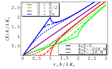
It is indeed seen in Fig. 5 that the behavior of the average drift velocity for is very different from . In the limiting case , we see that there is a critical current , in agreement with Eq. (19). In the large limit, we recognize a Walker-breakdown-like behavior, just like the behavior found in purely field-driven domain-wall motion. For very large currents, the drift velocity acquires a linear dependence on the spin current for all values of and for all temperatures.
III.2.2 Extrinsic pinning
Domain-wall pinning is of practical interest. Control of domain walls is achieved by pinning the domain wall in a position by means of, for example, a deformation in the material. In nanowires or thin metal strips, dents in the sample act as an intended pinning potential. A thorough understanding of depinning times is especially important in systems that are relevant for technological applications, such as data-storage devices.
To incorporate pinning in our theory, we add a pinning potential to the potential in Eqs. (24) and (25). A pinning potential that is due to a deformation in the material can be obtained through energy analysis. We discern between two types of deformations: symmetric and asymmetric notches. The sample we have in mind is a thin strip of ferromagnetic or semiconductor material, where the notches are little dents on the sides of the strip. In the case of symmetric notches, there is a dent on both sides of the sample. If there is only a dent on one side, we have an asymmetric notch. It turns out that symmetric pinning sites can effectively be described by a quadratic-well potential in the direction,[18] that is independent of the chirality. For asymmetric notches, the pinning potential also has a chirality dependence.[12]
As an example, we consider the symmetric notch. If we add a dependent symmetric-notch contribution to Eqs. (24) and (25), we see that the pinning contribution in Eq. (25) vanishes. Because of the explicit dependence in Eq. (24), the system can no longer be described by a probability distribution that depends on the variable only. Therefore, all terms in the Fokker-Planck equation (16) need to be taken into account, and we are not able to find an analytic solution to the full problem. We can, however, compute depinning times using Kramer’s escape-rate theory.
The potential that Tatara et al.[26] proposed for a symmetric notch has a kink at the sides, which makes it less suitable for escape-rate computations. We therefore use a very similar, but smooth potential
| (31) |
where is the depth and is the width of the potential well.
We compute depinning times for the pinning potential in Eq. (31) using Kramer’s escape-rate theory which states that the depinning time is proportional to , where is an attempt frequency and is the height of the potential barrier that has to be overcome. We determine the positions of the potential minimum and the saddle through variation of the potential . Substitution of these coordinates provides us with the potential difference . The depinning time for driving current and field is found as . Note that if , the depinning time is independent of the applied current within this approximation.
III.2.3 Disorder potential
The final potential that we consider is a disorder potential. Due to, for example, roughness on the edges of a sample, there is a random pinning potential that is felt by the domain wall. We consider a situation of strong pinning of the angle such that (See Ref. [23] for an extensive analysis including the dynamics of this angle). This would be the case for fields below Walker breakdown and currents below . The equation of motion for the coordinate is then found from Eq. (24) to be
| (32) |
The disorder potential that enters the equations of motion is characterized by certain spatial correlations . In this expression, the line denotes an average over the disorder, and is a measure for the strength of the disorder potential. The exponent characterizes the nature of the correlations. In general, there are two ways of obtaining a disorder potential: by applying a random field, or by randomizing locally the strength of certain coupling constants in the system, for example the anisotropy or the spin stiffness. The former is called random field disorder and gives rise to correlations with , whereas the latter is called random bond disorder with exponent . For both limits, Le Doussal and Vinokur[33] have obtained expressions for depinning times for a zero-dimensional object (in our one-dimensional model, the domain wall itself is described as a point at position with dimension zero).
For random field disorder (), Le Doussal and Vinokur find that the drift velocity is zero up to some critical driving current and/or field , and is then linear with the driving force
| (33) |
For random bond disorder () they find that the drift velocity obeys
| (34) |
where is the so-called dynamical exponent and is the gamma function. Surprisingly, they find that for the results turn out to resemble the results obtained for higher-dimensional objects, i.e. Le Doussal and Vinokur find a creep scaling law with a certain creep exponent
| (35) |
where is a characteristic critical driving force. Note that the creep exponent is always larger than for .
III.3 Comparison with other work
To compute drift velocities at finite temperature, we have expanded the theory proposed by Duine et al.[8] to include external magnetic fields in addition to driving currents. Other theoretical work is done by Tatara et al.[24] and by Martinez et al.[25] Here, we compare our results with the results by Martinez et al.
In order to write Eqs. (24) and (25) in terms of the coordinate only, Martinez et al. assume to be small such that . Note that this assumption only holds when and/or for . If, however, we do make this assumption, and differentiate Eqs. (24) and (25) with respect to time, we find
| (36) | ||||
| (37) |
where we omitted the stochastic terms. We now substitute Eqs. (24) and (37) in Eq. (36) and like Martinez et al. add a stochastic term to find
| (38) |
The correlations of the stochastic force are, according to Martinez et al., given by
| (39) |
From the fluctuation-dissipation theorem, they infer that . An easy way to obtain the Fokker-Planck equation is to introduce a new variable ,[27] such that we have two Langevin equations
| (40) | ||||
| (41) |
Note that the above equations have to be solved with the initial conditions to include the reactive spin-transfer torque. The Fokker-Planck equation generated by these Langevin equations is given by (we omit a factor )
| (42) |
This Fokker-Planck equation is satisfied by a Boltzmann equilibrium distribution that has the same potential energy as Eq. (26) for , but with an additional kinetic energy . The exact form of the stochastic strength is . We conclude that this procedure complies with our model for a small range of applicability.
Several field-driven domain-wall motion experiments have been performed in ferromagnetic metallic materials.[32, 18] Clear Walker-breakdown behavior is observed, but the peak is not smoothed like our theory predictions. Estimates by Duine et al.[22] show that room temperature, at which these experiments were performed, leads to an effective temperature for ferromagnetic metals. Our prediction is therefore indistinguishable from the zero-temperature curve in Fig. 4. The reason for this low effective temperature is the fact that the number of particles in the domain wall is relatively high in a ferromagnetic metal. In magnetic semiconductors, however, not all magnetic moments participate in the magnetization, reducing the number of magnetic moments in a domain wall by up to a factor , thereby greatly increasing the effective temperature. From Fig. 4 we see that an effective temperature should be distinguishable from the zero-temperature curve. We predict therefore that the influence of thermal effects on Walker breakdown should be observable with field-driven domain walls in clean magnetic semiconductors.
Escape time studies have been performed on narrow domain walls by Ravelosana et al.[13] They indeed find that the logarithm of the (average) escape time decreases linearly with the applied current. Since the current dependence of the logarithm of the escape time is determined by , we can estimate the value of from their curve, and we find that it is of the order , i.e. of the order of the damping parameter , in agreement with theoretical expectations.
IV Vortex domain walls
In this section we consider the limit of the domain-wall line that corresponds to vortex domain walls and derive several analytical and numerical results.
IV.1 Model
Vortex domain walls are described by making the ansatz for the dependence of the chirality
| (43) |
The coordinate plays a similar role as , and the width of the vortex domain wall in the direction is the equivalent of the width in the direction. The coordinates now determine the position of the vortex at time .
In principle, we should consider boundary conditions in the direction. We deal with this problem by assuming , in which limit the ansatz reduces to , with the Heaviside step function. The drawback is that we are now neglecting all boundary effects. The sign is the product of the chirality and charge in the ansatz and determines whether we have a clockwise or counterclockwise rotation in the vortex domain wall, and is usually denoted as the Skyrmion number . We note that the vortex domain wall is now fully characterized by its position , its dimensions , this Skyrmion number and the number of magnetic moments in the vortex .
We apply the simplified ansatz to the action in Eq. (9) to find an action for a vortex domain wall in terms of the collective coordinates and
| (44) | ||||
The dissipation function in Eq. (10) is also written in terms of the new coordinates, however, we need to take into account the full ansatz in Eq. (43) in order to find the dependence in the last term
| (45) |
Variation of the functionals in Eqs. (44) and (45) provides us with the Langevin equations for a vortex domain wall
| (46) | ||||
| (47) |
where we have again added stochastic forces to model thermal effects. We see that the effective dampings are given by and . We write the right-hand side of Eqs. (46) and (47) in terms of a total potential
| (48) |
Note that this potential is also obtained by inserting the ansatz in Eq. (15). With these identifications, we can again write the Langevin equations (46) and (47) in the more suggestive form
| (49) | ||||
| (50) |
Note that the prefactor is proportional to the inverse of the number of magnetic moments in the vortex domain wall. Using the Fokker-Planck method outlined in section II, we find that the probability distribution function does not satisfy Boltzmann equilibrium if we assume that the fluctuations in the and direction have the same strength. However, we write down a more general Fokker-Planck equation than the one in Eq. (16), in terms of stochastic correlations . Again, we demand the Boltzmann equilibrium in Eq (17) to be a solution to the modified Fokker-Planck equation, which yields complicated equations that can be solved. Up to second order in the small parameter , we find that the stochastic correlations must obey
| (51) |
where the indices denote and
| (52) |
In these relations, we recognize the fluctuation-dissipation theorem with effective temperature . The reduction by the factor is caused by the fact that the number of microscopic degrees of freedom is proportional to this factor. Note that, because the damping is anisotropic, it is also necessary to introduce anisotropy in the fluctuations.
From the form of Eqs. (49) and (50), it is clear that we reach the isotropic case for , i.e. when we demand that . Note that then also and that the reduction of the effective temperature is now proportional to . That this is indeed the isotropic case is also seen from the fact that now the coordinates and are treated on equal footing in the dissipation functional in Eq. (45).
If we also demand that , our model describes circular vortices, that furthermore occupy the entire width of the strip. This case is similar to the zero-temperature results of Shibata et al.[15] on the current-induced vortex displacement in a magnetic nanodisk, and their equations of motion correspond to ours in the case that and .
To include extrinsic pinning in our model, we again add a pinning potential to the potential . As an example, we will consider a circularly symmetric pinning potential, quadratic in both and , and bounded at a certain radius
| (53) |
IV.2 Results
IV.2.1 Zero temperature without extrinsic pinning
When there are no external fields or pinning potentials, we can read off the behavior directly from Eqs. (46) and (47). For instance, it is clear that under the influence of a current to the right, the domain wall will move to the right also, and its speed in the -direction will be directly proportional to the current, as can be seen in
| (54) |
Note that if , the velocity of the domain wall will be exactly equal to the velocity of the current. For the transverse velocity , we get
| (55) |
The direction of motion in the -direction depends on the skyrmion number , and also on the sign of , and the magnitude is proportional to . Theoretically, if , the vortex core would move in a straight line, i.e. the center of the vortex would not get a transverse displacement. Note that there is no intrinsic pinning in the case of a vortex domain wall, not even if . For , , showing that the shape of the vortex domain wall has an influence on the motion as well.
IV.2.2 Zero temperature with extrinsic pinning
We will now investigate what happens if there is a pinning potential of the form in Eq. (53). If the potential is not bounded (i.e. if the step function is absent), and , the solutions can be found analytically, and they describe a circular motion ending at a fixed point. As we can read from the formulas, these fixed points will be at and . Note that only the former depends on . This agrees with our physical intuition that tilts the potential landscape in the -direction, but that it has no effect in the -direction.
When the potential is bounded there is a critical current for depinning the domain wall. We cannot find this current precisely using analytic calculations, but we can however make a rough estimation if we take the current for which the equilibrium position falls outside the boundary as an indication. This will naturally overestimate the critical current since the domain wall precesses after the current is switched on, but it is a good approximation for the upper boundary. We find
| (56) |
Numerical calculations can give us more precise results. For instance, for a symmetric domain wall (i.e. ) with , , and , we find , while the analytical upper bound found with the formula above is . Numerical calculations also give us the escape time at , which is approximately (for ). Eq. (56) suggests that the critical current is proportional to . Fig. 6 shows both Eq. (56) and the numerical results for the aforementioned values of , and .

IV.2.3 Escape rate at finite temperature
We now include thermal fluctuations. To give some insight into the motion of the domain wall in this case, we have plotted a possible solution to the Langevin Eqs. (49) and (50) in Fig. 7. The current here is just under the critical one, , and we are looking at a symmetric vortex with .

We next determine the escape time (i.e. the time it takes for the domain wall to move outside the boundary of the pinning potential) as a function of the current, and its dependence on temperature. As the average escape time is rather hard to determine and as the escape times are distributed approximately exponentially, we have, for practical purposes, chosen the median escape time as an indicator. is then expected to be a good measure for the average escape time. The results, with the logarithm of the median escape time plotted against the current, are shown in Fig. 8.

Note that there is a clear distinction between the thermal regime and the slide regime. The behavior in the thermal regime can be fitted very well by an equation of the form , with and two numerical factors. Fitting shows to be of the order of , and around . Hence we find that the logarithm of the escape time is proportional to current.
IV.3 Comparison with other work
Vortex domain walls are of great interest to experimentalists, because they are large enough to be visible with, for instance, scanning electron microscopy or magnetic force microscopy, and because their dynamics take place on observable time scales. Because many experiments are done with vortex domain walls, many theoretical models have been developed to describe them. He, Li and Zhang[16] developed a 2D model for the vortex domain wall, while Shibata et al. [15] described the current-induced motion of a circular magnetic vortex. The biggest difference between these two models and ours is that in their case, the vortex (domain wall) is not straight, but the equations of motion they find are remarkably similar to ours in the isotropic, symmetric case. The former group found the motion of the domain wall towards the edge of the nanostrip that our model also yields, and the latter paper predicted precession of the vortex domain wall in a potential. The model of Krüger et al.[17] also predicts precession, of an elliptical shape, and our zero-temperature results are in agreement with theirs.
Current-driven vortex domain wall motion has indeed been observed by several experimental groups.[20, 34, 35] Furthermore, Heyne et al. [7] found, as expected, that the sign of the displacement in the -direction is determined by the skyrmion number and by the sign of . In the presence of pinning, precession of a magnetic vortex has indeed been found experimentally as well.[19]
No detailed experimental results on current-driven magnetic vortices at nonzero temperature have been reported.
V Conclusions
We have presented a model for the driven motion of a domain-wall line at nonzero temperature, and analyzed this model within several approximations.
First, we considered a general domain-wall line, which is described as a string in a tilted washboard potential. We computed the average drift velocity as a function of an applied current for currents lower than the critical current.
In the limit of rigid domain walls, we were able to find analytical expressions for drift velocities in the presence of thermal fluctuations. For the field-driven case, the well-known Walker-breakdown behavior smoothes for increasing temperature. In the current-driven case, the drift velocity depends heavily on the ratio of the dissipative spin-transfer torque parameter and the Gilbert damping . Here, the curves also smoothen with increasing temperature. As a result, we found no critical current for at nonzero temperature. We also considered extrinsic pinning due to, for example, a notch in the sample. We found that the escape time is proportional to the exponent of the applied magnetic field and the dissipative spin-transfer torque. Comparison with experiment enabled us to estimate for that experiment[13]. Finally, we discussed the effect of a disorder potential on the dynamics of the rigid domain wall.
For vortex domain walls, we computed domain-wall velocities at zero temperature. In the presence of an extrinsic pinning potential, we found an analytic upper bound for the critical current. Numerical computation revealed critical currents just under this upper bound. At finite temperature, numerical simulations provided us with depinning times as a function of the applied current. We found two distinct regimes: one where thermal fluctuations dominate, and one where the current dominates. In the thermal regime, we found that the depinning time goes as .
The models and results presented in this paper provide a simple framework for describing domain walls at nonzero temperature. Moreover, they are easily adapted to situations not discussed in this paper, such as different geometries. We hope that our results are confirmed with more experimental and numerical results in the near future.
Acknowledgements.
This work was supported by the Netherlands Organization for Scientific Research (NWO), by the European Research Council (ERC) under the Seventh Framework Program (FP7), and by the National Science Foundation under Grant No. NSF PHY05-51164.References
- [1] L. Berger, J. Appl. Phys. 55, 1954 (1984).
- [2] P.P. Freitas and L. Berger, J. Appl. Phys. 57, 1266 (1985).
- [3] J.C. Slonczewski, J. Magn. Magn. Mater. 159, L1 (1996).
- [4] L. Berger, Phys. Rev. B. 54, 9353 (1996).
- [5] S. Zhang and Z. Li, Phys. Rev. Lett. 93, 127204 (2004).
- [6] S.E. Barnes and S. Maekawa, Phys. Rev. Lett. 95, 107204 (2005).
- [7] L. Heyne et al., Phys. Rev. Lett. 100, 066603 (2008).
- [8] R.A. Duine, A.D. Núñez, J. Sinova and A. H. MacDonald, Phys. Rev. B 75, 214420 (2007).
- [9] T. Tserkovnyak, H.J. Skadsem, A. Brataas and G.E.W. Bauer, Phys. Rev. B 74, 144405 (2006).
- [10] H. Kohno, G. Tatara and J. Shibata, J. Phys. Soc. Jpn. 75, 113706 (2006).
- [11] F. Piéchon and A. Thiaville, Phys. Rev. B 75, 174414 (2007).
- [12] D. Petit, A.-V. Jausovec, D. Read, and R.P. Cowburn, J. Appl. Phys. 103, 114307 (2008).
- [13] D. Ravelosona, D. Lacour, J. A. Katine, B. D. Terris and C. Chappert, Phys. Rev. Lett. 95, 117203 (2005).
- [14] P. Bruno, Phys. Rev. Lett. 83, 2425 (1999).
- [15] J. Shibata, Y. Nakatani, G. Tatara, H. Kohno and Y. Otani, Phys. Rev. B 73, 020403 (R) (2006).
- [16] J.He, Z.Li and S. Zhang, Phys. Rev. B. 73, 184408 (2006).
- [17] B. Krüger, A. Drews, M. Bolte, U. Merkt, D. Pfannkuche and G. Meier, Phys. Rev. B 76, 224426 (2007).
- [18] M. Hayashi, L. Thomas, C. Rettner, R. Moriya, X. Jiang, and S.S.P. Parkin, Phys. Rev. Lett. 97, 207205 (2006).
- [19] M. Bolte et al., Phys. Rev. Lett. 100, 176601 (2008).
- [20] M. Kläui, P.-O. Jubert, R. Allenspach, A. Bischof, J. A. C. Bland, G. Faini, U. Rüdiger, C. A. F. Vaz, L. Vila and C. Vouille, Phys. Rev. Lett. 95, 026601 (2005).
- [21] R.A. Duine and C. Morais Smith, Phys. Rev. B 77, 094434 (2008).
- [22] R.A. Duine, A.S. Núñez and A.H. MacDonald, Phys. Rev. Lett. 98, 056605 (2007).
- [23] V. Lecomte, S.E. Barnes, J.-P. Eckmann and T. Giamarchi, cond-mat.stat-mech/0903.0175 (2009).
- [24] G. Tatara, N. Vernier and J. Ferré, Appl. Phys. Lett. 86, 252509 (2005).
- [25] E. Martinez, L. Lopez-Diaz, O. Alejos, L. Torres and C. Tristan, Phys. Rev. Lett. 98, 267202 (2007).
- [26] G. Tatara and H. Kohno, Phys. Rev. Lett. 92, 086601 (2004); 96, 189702 (2006).
- [27] H. Risken, The Fokker-Planck Equation (Springer-Verlag, Berlin, 1984).
- [28] M. Büttiker and R. Landauer, Phys. Rev. A 23, 1397 (1981).
- [29] M. Yamanouchi, J. Ieda, F. Matsukura, S. E. Barnes, S. Maekawa, H. Ohno, Science 317, 1726 (2007).
- [30] T.A. Moore, I.M. Miron, G. Gaudin, G. Serret, S. Auffret, B. Rodmacq, A. Schuhl, S. Pizzini, J. Vogel and M. Bonfim, cond-mat.other/0812.1515 (2008).
- [31] N.L. Schryer and L.R. Walker, J. Appl. Phys. 45, 5406 (1974).
- [32] G.S.D. Beach, C. Nistor, C. Knutson, M. Tsoi and J.L. Erskine, Nature Mat. 4, 741 (2005).
- [33] P. Le Doussal and V.M. Vinokur, Physica C 254, 63 (1995).
- [34] A. Yamaguchi, T. Ono, S. Nasu, K. Miyake, K. Mibu and T. Shinjo, Phys. Rev. Lett. 92, 077205 (2004).
- [35] L. Thomas, M. Hayashi, X. Jiang, R. Moriya, C. Rettner and S.S.P. Parkin, Nature 443, 197 (2006).