Modified-CS: Modifying Compressive Sensing for Problems with Partially Known Support Thanks: N. Vaswani and W. Lu are with the ECE dept. at Iowa State University (email: {namrata,luwei}@iastate.edu). A part of this work appeared in [1, 2]. This research was supported by NSF grants ECCS-0725849 and CCF-0917015. Copyright (c) 2010 IEEE. Personal use of this material is permitted. However, permission to use this material for any other purposes must be obtained from the IEEE by sending a request to pubs-permissions@ieee.org.

Namrata Vaswani Wei Lu

Abstract

We study the problem of reconstructing a sparse signal from a limited number of its linear projections when a part of its support is known, although the known part may contain some errors. The “known” part of the support, denoted $T$ , may be available from prior knowledge. Alternatively, in a problem of recursively reconstructing time sequences of sparse spatial signals, one may use the support estimate from the previous time instant as the “known” part. The idea of our proposed solution (modified-CS) is to solve a convex relaxation of the following problem: find the signal that satisfies the data constraint and is sparsest outside of $T$ . We obtain sufficient conditions for exact reconstruction using modified-CS. These are much weaker than those needed for compressive sensing (CS) when the sizes of the unknown part of the support and of errors in the known part are small compared to the support size. An important extension called Regularized Modified-CS (RegModCS) is developed which also uses prior signal estimate knowledge. Simulation comparisons for both sparse and compressible signals are shown.

I Introduction

In this work, we study the sparse reconstruction problem from noiseless measurements when a part of the support is known, although the known part may contain some errors. The “known” part of the support may be available from prior knowledge. For example, consider MR image reconstruction using the 2D discrete wavelet transform (DWT) as the sparsifying basis. If it is known that an image has no (or very little) black background, all (or most) approximation coefficients will be nonzero. In this case, the “known support” is the set of indices of the approximation coefficients. Alternatively, in a problem of recursively reconstructing time sequences of sparse spatial signals, one may use the support estimate from the previous time instant as the “known support”. This latter problem occurs in various practical applications such as real-time dynamic MRI reconstruction, real-time single-pixel camera video imaging or video compression/decompression. There are also numerous other potential applications where sparse reconstruction for time sequences of signals/images may be needed, e.g. see [3, 4].

Refer to caption — (a) Top: larynx image sequence, Bottom: cardiac sequence

Sparse reconstruction has been well studied for a while, e.g. see [5, 6]. Recent work on Compressed Sensing (CS) gives conditions for its exact reconstruction [7, 8, 9] and bounds the error when this is not possible [10, 11].

Our recent work on Least Squares CS-residual (LS-CS) [12, 13] can be interpreted as a solution to the problem of sparse reconstruction with partly known support. LS-CS replaces CS on the observation by CS on the LS observation residual, computed using the “known” part of the support. Since the observation residual measures the signal residual which has much fewer large nonzero components, LS-CS greatly improves reconstruction error when fewer measurements are available. But the exact sparsity size (total number of nonzero components) of the signal residual is equal to or larger than that of the signal. Since the number of measurements required for exact reconstruction is governed by the exact sparsity size, LS-CS is not able to achieve exact reconstruction using fewer noiseless measurements than those needed by CS.

Exact reconstruction using fewer noiseless measurements than those needed for CS is the focus of the current work. Denote the “known” part of the support by $T$ . Our proposed solution (modified-CS) solves an $\ell_{1}$ relaxation of the following problem: find the signal that satisfies the data constraint and is sparsest outside of $T$ . We derive sufficient conditions for exact reconstruction using modified-CS. When $T$ is a fairly accurate estimate of the true support, these are much weaker than the sufficient conditions for CS. For a recursive time sequence reconstruction problem, this holds if the reconstruction at $t=0$ is exact and the support changes slowly over time. The former can be ensured by using more measurements at $t=0$ , while the latter is often true in practice, e.g. see Fig. 1.

We also develop an important extension called Regularized Modified-CS which also uses prior signal estimate knowledge. It improves the error when exact reconstruction is not possible.

A shorter version of this work first appeared in ISIT’09 [1]. In parallel and independent work in [14], Khajehnejad et al have also studied a similar problem to ours but they assume a probabilistic prior on the support. Other related work includes [15]. Very recent work on causal reconstruction of time sequences includes [16] (focusses on the time-invariant support case) and [17] (use past estimates to only speed up the current optimization but not to improve reconstruction error). Except [14], none of these prove exact reconstruction using fewer measurements and except [15, 14], none of these even demonstrate it.

Other recent work, e.g. [18], applies CS on observation differences to reconstruct the difference signal. While their goal is to only estimate the difference signal, the approach could be easily modified to also reconstruct the actual signal sequence (we refer to this as CS-diff). But, since all nonzero coefficients of a sparse signal in any sparsity basis will typically change over time, though gradually, and some new elements will become nonzero, thus the exact sparsity size of the signal difference will also be equal to/larger than that of the signal itself. As a result CS-diff will also not achieve exact reconstruction using fewer measurements, e.g. see Fig.3.

In this work, whenever we use the term CS, we are actually referring to basis pursuit (BP) [5]. As pointed out by an anonymous reviewer, modified-CS is a misnomer and a more appropriate name for our approach should be modified-BP.

As pointed out by an anonymous reviewer, modified-CS can be used in conjunction with multiscale CS for video compression [19] to improve their compression ratios.

The paper is organized as follows. We give the notation and problem definition below. Modified-CS is developed in Sec. II. We obtain sufficient conditions for exact reconstruction using it in Sec. III. In Sec. IV, we compare these with the corresponding conditions for CS and we also do a Monte Carlo comparison of modified-CS and CS. We discuss Dynamic Modified-CS and Regularized Modified CS in Sec. V. Comparisons for actual images and image sequences are given in Sec. VI and conclusions and future work in Sec. VII.

I-A Notation

We use ^′ for transpose. The notation $\|c\|_{k}$ denotes the $\ell_{k}$ norm of the vector $c$ . The $\ell_{0}$ pseudo-norm, $\|c\|_{0}$ , counts the number of nonzero elements in $c$ . For a matrix, $M$ , $\|M\|$ denotes its induced $\ell_{2}$ norm, i.e. $\|M\|:=\max_{c:\|c\|_{2}=1}\|Mc\|_{2}$ .

We use the notation $A_{T}$ to denote the sub-matrix containing the columns of $A$ with indices belonging to $T$ . For a vector, the notation $(\beta)_{T}$ (or $\beta_{T}$ ) refers to a sub-vector that contains the elements with indices in $T$ . The notation, $[1,n]:=[1,2,\dots n]$ . We use $T^{c}$ to denote the complement of the set $T$ w.r.t. $[1,n]$ , i.e. $T^{c}:=[1,n]\setminus T$ . The set operations, $\cup,\cap$ stand for set union and intersection respectively. Also $T_{1}\setminus T_{2}:=T_{1}\cap T_{2}^{c}$ denotes set difference. For a set $T$ , $|T|$ denotes its size (cardinality). But for a scalar, $b$ , $|b|$ denotes the magnitude of $b$ .

The $S$ -restricted isometry constant [9], $\delta_{S}$ , for a matrix, $A$ , is defined as the smallest real number satisfying

\displaystyle(1-\delta_{S})\|c\|_{2}^{2}\leq\|A_{T}c\|_{2}^{2}\leq(1+\delta_{S})\|c\|_{2}^{2}

(1)

for all subsets $T\subset[1,n]$ of cardinality $|T|\leq S$ and all real vectors $c$ of length $|T|$ . The restricted orthogonality constant [9], $\theta_{S_{1},S_{2}}$ , is defined as the smallest real number satisfying

\displaystyle|{c_{1}}^{\prime}{A_{T_{1}}}^{\prime}A_{T_{2}}c_{2}|\leq\theta_{S_{1},S_{2}}\|c_{1}\|_{2}\|c_{2}\|_{2}

(2)

for all disjoint sets $T_{1},T_{2}\subset[1,n]$ with $|T_{1}|\leq S_{1}$ , $|T_{2}|\leq S_{2}$ and $S_{1}+S_{2}\leq n$ , and for all vectors $c_{1}$ , $c_{2}$ of length $|T_{1}|$ , $|T_{2}|$ respectively. By setting $c_{1}\equiv{A_{T_{1}}}^{\prime}A_{T_{2}}c_{2}$ in (2),

\displaystyle\|{A_{T_{1}}}^{\prime}A_{T_{2}}\|\leq\theta_{S_{1},S_{2}}

(3)

The notation $X\sim{\cal N}(\mu,\Sigma)$ means that $X$ is Gaussian distributed with mean $\mu$ and covariance $\Sigma$ while ${\cal N}(x;\mu,\Sigma)$ denotes the value of the Gaussian PDF computed at point $x$ .

I-B Problem Definition

We measure an $m$ -length vector $y$ where

\displaystyle y:=Ax

(4)

We need to estimate $x$ which is a sparse $n$ -length vector with $n>m$ . The support of $x$ , denoted $N$ , can be split as $N=T\cup\Delta\setminus\Delta_{e}$ where $T$ is the “known” part of the support, $\Delta_{e}:=T\setminus N$ is the error in the the known part and $\Delta:=N\setminus T$ is the unknown part. Thus, $\Delta_{e}\subseteq T$ , $\Delta$ , $T$ are disjoint and $|N|=|T|+|\Delta|-|\Delta_{e}|$ .

We use $s:=|N|$ to denote the size of the (s)upport, $k:=|T|$ to denote the size of the (k)nown part of the support, $e=|\Delta_{e}|$ to denote the size of the (e)rror in the known part and $u=|\Delta|$ to denote the size of the (u)nknown part of the support.

We assume that $A$ satisfies the $S$ -restricted isometry property (RIP) [9] for $S=(s+e+u)=(k+2u)$ . $S$ -RIP means that $\delta_{S}<1$ where $\delta_{S}$ is the RIP constant for $A$ defined in (1).

In a static problem, $T$ is available from prior knowledge. For example, in the MRI problem described in the introduction, let $N$ be the (unknown) set of all DWT coefficients with magnitude above a certain zeroing threshold. Assume that the smaller coefficients are set to zero. Prior knowledge tells us that most image intensities are nonzero and so the approximation coefficients are mostly nonzero. Thus we can let $T$ be the (known) set of indices of all the approximation coefficients. The (unknown) set of indices of the approximation coefficients which are zero form $\Delta_{e}$ . The (unknown) set of indices of the nonzero detail coefficients form $\Delta$ .

For the time series problem, $y\equiv y_{t}$ and $x\equiv x_{t}$ with support, $N_{t}=T\cup\Delta\setminus\Delta_{e}$ , and $T=\hat{N}_{t-1}$ is the support estimate from the previous time instant. If exact reconstruction occurs at $t-1$ , $T=N_{t-1}$ . In this case, $\Delta_{e}=N_{t-1}\setminus N_{t}$ is the set of indices of elements that were nonzero at $t-1$ , but are now zero (deletions) while $\Delta=N_{t}\setminus N_{t-1}$ is the newly added coefficients at $t$ (additions). Slow sparsity pattern change over time, e.g. see Fig. 1, then implies that $u\equiv|\Delta|$ and $e\equiv|\Delta_{e}|$ are much smaller than $s\equiv|N|$ .

When exact reconstruction does not occur, $\Delta_{e}$ includes both the current deletions and the extras from $t-1$ , $\hat{N}_{t-1}\setminus N_{t-1}$ . Similarly, $\Delta$ includes both the current additions and the misses from $t-1$ , $N_{t-1}\setminus\hat{N}_{t-1}$ . In this case, slow support change, along with $\hat{N}_{t-1}\approx N_{t-1}$ , still implies that $u\ll s$ and $e\ll s$ .

II Modified Compressive Sensing (modified-CS)

Our goal is to find a signal that satisfies the data constraint given in (4) and whose support contains the smallest number of new additions to $T$ , although it may or may not contain all elements of $T$ . In other words, we would like to solve

\displaystyle\min_{\beta}\|(\beta)_{T^{c}}\|_{0}\ \text{subject to}\ y=A\beta

(5)

If $\Delta_{e}$ is empty, i.e. if $N=T\cup\Delta$ , then the solution of (5) is also the sparsest solution whose support contains $T$ .

As is well known, minimizing the $\ell_{0}$ norm is a combinatorial optimization problem [20]. We propose to use the same trick that resulted in CS [5, 7, 8, 10]. We replace the $\ell_{0}$ norm by the $\ell_{1}$ norm, which is the closest norm to $\ell_{0}$ that makes the optimization problem convex, i.e. we solve

\displaystyle\min_{\beta}\|(\beta)_{T^{c}}\|_{1}\ \text{subject to}\ y=A\beta

(6)

Denote its output by $\hat{x}$ . If needed, the support can be estimated as

\displaystyle\hat{N}:=\{i\in[1,n]:(\hat{x})_{i}^{2}>\alpha\}

(7)

where $\alpha\geq 0$ is a zeroing threshold. If exact reconstruction occurs, $\alpha$ can be zero. We discuss threshold setting for cases where exact reconstruction does not occur in Sec. V-A.

III Exact Reconstruction Result

We first analyze the $\ell_{0}$ version of modified-CS in Sec. III-A. We then give the exact reconstruction result for the actual $\ell_{1}$ problem in Sec. III-B. In Sec. III-C, we give the two key lemmas that lead to its proof and we explain how they lead to the proof. The complete proof is given in the Appendix. The proof of the lemmas is given in Sec. III-D.

Recall that $k=|T|$ , $u=|\Delta|$ , $e=|\Delta_{e}|$ and $s=|N|$ .

III-A Exact Reconstruction Result: $\ell_{0}$ version of modified-CS

Consider the $\ell_{0}$ problem, (5). Using a rank argument similar to [9, Lemma 1.2] we can show the following. The proof is given in the Appendix.

Proposition 1

Given a sparse vector, $x$ , with support, $N=T\cup\Delta\setminus\Delta_{e}$ , where $\Delta$ and $T$ are disjoint and $\Delta_{e}\subseteq T$ . Consider reconstructing it from $y:=Ax$ by solving (5). $x$ is the unique minimizer of (5) if $\delta_{k+2u}<1$ ( $A$ satisfies the $(k+2u)$ -RIP).

Using $k=s+e-u$ , this is equivalent to $\delta_{s+e+u}<1$ . Compare this with [9, Lemma 1.2] for the $\ell_{0}$ version of CS. It requires $\delta_{2s}<1$ which is much stronger when $u\ll s$ and $e\ll s$ , as is true for time series problems.

III-B Exact Reconstruction Result: modified-CS

Of course we do not solve (5) but its $\ell_{1}$ relaxation, (6). Just like in CS, the sufficient conditions for this to give exact reconstruction will be slightly stronger. In the next few subsections, we prove the following result.

Theorem 1 (Exact Reconstruction)

Given a sparse vector, $x$ , whose support, $N=T\cup\Delta\setminus\Delta_{e}$ , where $\Delta$ and $T$ are disjoint and $\Delta_{e}\subseteq T$ . Consider reconstructing it from $y:=Ax$ by solving (6). $x$ is the unique minimizer of (6) if

1.

$\delta_{k+u}<1$ and $\delta_{2u}+\delta_{k}+\theta_{k,2u}^{2}<1$ and

$a_{k}(2u,u)+a_{k}(u,u)<1$ where

\displaystyle a_{k}(S,\check{S})

\displaystyle:=

\displaystyle\frac{\theta_{\check{S},S}+\frac{\theta_{\check{S},k}\ \theta_{S,k}}{1-\delta_{k}}}{1-\delta_{S}-\frac{\theta_{S,k}^{2}}{1-\delta_{k}}}

(8)

The above conditions can be rewritten using $k=s+e-u$ .

To understand the second condition better and relate it to the corresponding CS result, let us simplify it. $a_{k}(2u,u)+a_{k}(u,u)\leq\frac{\theta_{u,2u}+\theta_{u,u}+\frac{\theta_{2u,k}^{2}+\theta_{u,k}^{2}}{1-\delta_{k}}}{1-\delta_{2u}-\frac{\theta_{2u,k}^{2}}{1-\delta_{k}}}.$ Simplifying further, a sufficient condition for $a_{k}(2u,u)+a_{k}(u,u)<1$ is $\theta_{u,2u}+\theta_{u,u}+\frac{2\theta_{2u,k}^{2}+\theta_{u,k}^{2}}{1-\delta_{k}}+\delta_{2u}<1$ . Further, a sufficient condition for this is $\theta_{u,u}+\delta_{2u}+\theta_{u,2u}+\delta_{k}+\theta_{u,k}^{2}+2\theta_{2u,k}^{2}<1$ .

To get a condition only in terms of $\delta_{S}$ ’s, use the fact that $\theta_{S,\check{S}}\leq\delta_{S+\check{S}}$ [9]. A sufficient condition is $2\delta_{2u}+\delta_{3u}+\delta_{k}+\delta_{k+u}^{2}+2\delta_{k+2u}^{2}<1$ . Further, notice that if $u\leq k$ and if $\delta_{k+2u}<1/5$ , then $2\delta_{2u}+\delta_{3u}+\delta_{k}+\delta_{k+u}^{2}+2\delta_{k+2u}^{2}<4\delta_{k+2u}+\delta_{k+2u}(3\delta_{k+2u})\leq(4+3/5)\delta_{k+2u}<23/25<1$ .

Corollary 1 (Exact Reconstruction)

•

$x$ is the unique minimizer of (6) if $\delta_{k+u}<1$ and

$\displaystyle(\delta_{2u}+\theta_{u,u}+\theta_{u,2u})+(\delta_{k}+\theta_{k,u}^{2}+2\theta_{k,2u}^{2})<1$ (9)
•

This, in turn, holds if

$2\delta_{2u}+\delta_{3u}+\delta_{k}+\delta_{k+u}^{2}+2\delta_{k+2u}^{2}<1.$
•

This, in turn, holds if $u\leq k$ and

$\delta_{k+2u}<1/5.$

These conditions can be rewritten by substituting $k=s+e-u$ .

Compare (9) to the sufficient condition for CS given in [9]:

\displaystyle\delta_{2s}+\theta_{s,s}+\theta_{s,2s}<1

(10)

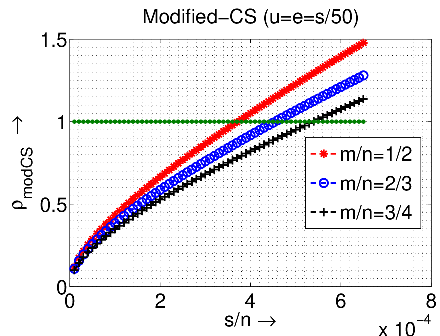
As shown in Fig. 1, usually $u\ll s$ , $e\ll s$ and $u\approx e$ (which means that $k\approx s$ ). Consider the case when the number of measurements, $m$ , is smaller than what is needed for exact reconstruction for a given support size, $s$ , but is large enough to ensure that $\theta_{k,2u}<1/2$ . Under these assumptions, compare (9) with (10). Notice that (a) the first bracket of the left hand side (LHS) of (9) will be small compared to the LHS of (10). The same will hold for the second and third terms of its second bracket compared with the second and third terms of (10). The first term of its second bracket, $\delta_{k}$ , will be smaller than the first term of (10), $\delta_{2s}$ . Thus, for a certain range of values of $m$ , the LHS of (9) will be smaller than that of (10) and it may happen that (9) holds, but (10) does not hold. For example, if $m<2s$ , (10) will not hold, but if $s+u+e<m<2s$ , (9) can hold if $u,e$ are small enough. A detailed comparison is done in Sec. IV.

III-C Proof of Theorem 1: Main Lemmas and Proof Outline

The idea of the proof is motivated by that of [9, Theorem 1.3]. Suppose that we want to minimize a convex function $J(\beta)$ subject to $A\beta=y$ and that $J$ is differentiable. The Lagrange multiplier optimality condition requires that there exists a Lagrange multiplier, $w$ , s.t. $\nabla J(\beta)-A^{\prime}w=0$ . Thus for $x$ to be a solution we need $A^{\prime}w=\nabla J(x)$ . In our case, $J(x)=\|x_{T^{c}}\|_{1}=\sum_{j\in T^{c}}|x_{j}|$ . Thus $(\nabla J(x))_{j}=0$ for $j\in T$ and $(\nabla J(x))_{j}=\text{sgn}(x_{j})$ for $j\in\Delta$ . For $j\notin T\cup\Delta$ , $x_{j}=0$ . Since $J$ is not differentiable at 0, we require that $(A^{\prime}w)_{j}={A_{j}}^{\prime}w=w^{\prime}A_{j}$ lie in the subgradient set of $J(x_{j})$ at 0, which is the set $[-1,1]$ [21]. In summary, we need a $w$ that satisfies

	$\displaystyle w^{\prime}A_{j}$	$\displaystyle=$	$\displaystyle 0\ \text{if}\ j\in T,\ \ w^{\prime}A_{j}=\text{sgn}(x_{j})\ \text{if}\ j\in\Delta,\ \text{and}$
	$\displaystyle\|w^{\prime}A_{j}\|$	$\displaystyle\leq$	$\displaystyle 1,\ \text{if}\ j\notin T\cup\Delta$		(11)

Lemma 1 below shows that by using (11) but with $|w^{\prime}A_{j}|\leq 1$ replaced by $|w^{\prime}A_{j}|<1$ for all $j\notin T\cup\Delta$ , we get a set of sufficient conditions for $x$ to be the unique solution of (6).

Lemma 1

The sparse signal, $x$ , with support as defined in Theorem 1, and with $y:=Ax$ , is the unique minimizer of (6) if $\delta_{k+u}<1$ and if we can find a vector $w$ satisfying

1.

$w^{\prime}A_{j}=0\ \text{if}\ j\in T$
2.

$w^{\prime}A_{j}=\text{sgn}(x_{j})\ \text{if}\ j\in\Delta$
3.

$|w^{\prime}A_{j}|<1,\ \text{if}\ j\notin T\cup\Delta$

Recall that $k=|T|$ and $u=|\Delta|$ .

The proof is given in the next subsection.

Next we give Lemma 2 which constructs a $\tilde{w}$ which satisfies ${A_{T}}^{\prime}\tilde{w}=0$ and ${A_{T_{d}}}^{\prime}\tilde{w}=c$ for any set $T_{d}$ disjoint with $T$ of size $|T_{d}|\leq S$ and for any given vector $c$ of size $|T_{d}|$ . It also bounds $|{A_{j}}^{\prime}\tilde{w}|$ for all $j\notin T\cup T_{d}\cup E$ where $E$ is called an “exceptional set”. We prove Theorem 1 by applying Lemma 2 iteratively to construct a $w$ that satisfies the conditions of Lemma 1 under the assumptions of Theorem 1.

Lemma 2

Given the known part of the support, $T$ , of size $k$ . Let $S$ , $\check{S}$ be such that $k+S+\check{S}\leq n$ and $\delta_{S}+\delta_{k}+\theta_{k,S}^{2}<1$ . Let $c$ be a vector supported on a set $T_{d}$ , that is disjoint with $T$ , of size $|T_{d}|\leq S$ . Then there exists a vector $\tilde{w}$ and an exceptional set, $E$ , disjoint with $T\cup T_{d}$ , s.t.

$\displaystyle{A_{j}}^{\prime}\tilde{w}$	$\displaystyle=$	$\displaystyle 0,\ \forall\ j\in T$
$\displaystyle{A_{j}}^{\prime}\tilde{w}$	$\displaystyle=$	$\displaystyle c_{j},\ \forall\ j\in T_{d}$	(12)
$\displaystyle\|E\|$	$\displaystyle<$	$\displaystyle\check{S}$
$\displaystyle\\|{A_{E}}^{\prime}\tilde{w}\\|_{2}$	$\displaystyle\leq$	$\displaystyle a_{k}(S,\check{S})\\|c\\|_{2}$
$\displaystyle\|{A_{j}}^{\prime}\tilde{w}\|$	$\displaystyle\leq$	$\displaystyle\frac{a_{k}(S,\check{S})}{\sqrt{\check{S}}}\\|c\\|_{2}\ \forall j\notin T\cup T_{d}\cup E\ \ \text{and}$
$\displaystyle\\|\tilde{w}\\|_{2}$	$\displaystyle\leq$	$\displaystyle K_{k}(S)\\|c\\|_{2}$	(13)

where $a_{k}(S,\check{S})$ is defined in (8) and

\displaystyle K_{k}(S)

\displaystyle:=

\displaystyle\frac{\sqrt{1+\delta_{S}}}{1-\delta_{S}-\frac{\theta_{S,k}^{2}}{1-\delta_{k}}}

(14)

The proof is given in the next subsection.

Proof Outline of Theorem 1. To prove Theorem 1, apply Lemma 2 iteratively, in a fashion similar to that of the proof of [9, Lemma 2.2] (this proof had some important typos). The main idea is as follows. At iteration zero, apply Lemma 2 with $T_{d}\equiv\Delta$ (so that $S\equiv u$ ), $c_{j}\equiv\text{sgn}(x_{j})\ \forall\ j\in\Delta$ , and $\check{S}\equiv u$ , to get a $w_{1}$ and an exceptional set $T_{d,1}$ , of size less than $u$ , that satisfy the above conditions. At iteration $r>0$ , apply Lemma 2 with $T_{d}\equiv\Delta\cup T_{d,r}$ (so that $S\equiv 2u$ ), $c_{j}\equiv 0\ \forall\ j\in\Delta$ , $c_{j}\equiv{A_{j}}^{\prime}w_{r}\ \forall\ j\in T_{d,r}$ and $\check{S}\equiv u$ to get a $w_{r+1}$ and an exceptional set $T_{d,r+1}$ , of size less than $u$ . Lemma 2 is applicable in the above fashion because condition 1 of Theorem 1 holds. Define $w:=\sum_{r=1}^{\infty}(-1)^{r-1}w_{r}$ . We then argue that if condition 2 of Theorem 1 holds, $w$ satisfies the conditions of Lemma 1. Applying Lemma 1, the result follows. We give the entire proof in the Appendix.

III-D Proofs of Lemmas 1 and 2

We prove the lemmas from the previous subsection here. Recall that $k=|T|$ and $u=|\Delta|$ .

III-D1 Proof of Lemma 1

The proof is motivated by [9, Section II-A]. There is clearly at least one element in the feasible set of (6) - $x$ - and hence there will be at least one minimizer of (6). Let $\beta$ be a minimizer of (6). We need to prove that if the conditions of the lemma hold, it is equal to $x$ . For any minimizer, $\beta$ ,

\displaystyle\|(\beta)_{T^{c}}\|_{1}\leq\|(x)_{T^{c}}\|_{1}:=\sum_{j\in\Delta}|x_{j}|

(15)

Recall that $x$ is zero outside of $T\cup\Delta$ , $T$ and $\Delta$ are disjoint, and $x$ is always nonzero on the set $\Delta$ . Take a $w$ that satisfies the three conditions of the lemma. Then,

$\displaystyle\\|(\beta)_{T^{c}}\\|_{1}$	$\displaystyle=$	$\displaystyle\sum_{j\in\Delta}\|x_{j}+(\beta_{j}-x_{j})\|+\sum_{j\notin T\cup\Delta}\|\beta_{j}\|$	(16)
	$\displaystyle\geq$	$\displaystyle\sum_{j\in\Delta}\|x_{j}+(\beta_{j}-x_{j})\|+\sum_{j\notin T\cup\Delta}w^{\prime}A_{j}\beta_{j}$
	$\displaystyle\geq$	$\displaystyle\sum_{j\in\Delta}\text{sgn}(x_{j})(x_{j}+(\beta_{j}-x_{j}))+\sum_{j\notin T\cup\Delta}w^{\prime}A_{j}\beta_{j}$
	$\displaystyle=$	$\displaystyle\sum_{j\in\Delta}\|x_{j}\|+\sum_{j\in\Delta}w^{\prime}A_{j}(\beta_{j}-x_{j})+\sum_{j\notin T\cup\Delta}w^{\prime}A_{j}\beta_{j}$
		$\displaystyle+\sum_{j\in T}w^{\prime}A_{j}(\beta_{j}-x_{j})$
	$\displaystyle=$	$\displaystyle\\|x_{T^{c}}\\|_{1}+w^{\prime}(A\beta-Ax)=\\|x_{T^{c}}\\|_{1}$

Now, the only way (16) and (15) can hold simultaneously is if all inequalities in (16) are actually equalities. Consider the first inequality. Since $|w^{\prime}A_{j}|$ is strictly less than 1 for all $j\notin T\cup\Delta$ , the only way $\sum_{j\notin T\cup\Delta}|\beta_{j}|=\sum_{j\notin T\cup\Delta}w^{\prime}A_{j}\beta_{j}$ is if $\beta_{j}=0$ for all $j\notin T\cup\Delta$ .

Since both $\beta$ and $x$ solve (6), $y=Ax=A\beta$ . Since $\beta_{j}=0=x_{j}$ for all $j\notin T\cup\Delta$ , this means that $y=A_{T\cup\Delta}(\beta)_{T\cup\Delta}=A_{T\cup\Delta}(x)_{T\cup\Delta}$ or that $A_{T\cup\Delta}((\beta)_{T\cup\Delta}-(x)_{T\cup\Delta})=0$ . Since $\delta_{k+u}<1$ , $A_{T\cup\Delta}$ is full rank and so the only way this can happen is if $(\beta)_{T\cup\Delta}=(x)_{T\cup\Delta}$ . Thus any minimizer, $\beta=x$ , i.e. $x$ is the unique minimizer of (6). $\blacksquare$

III-D2 Proof of Lemma 2

The proof of this lemma is significantly different from that of the corresponding lemma in [9], even though the form of the final result is similar.

Any $\tilde{w}$ that satisfies ${A_{T}}^{\prime}\tilde{w}=0$ will be of the form

\displaystyle\tilde{w}=[I-A_{T}({A_{T}}^{\prime}A_{T})^{-1}{A_{T}}^{\prime}]\gamma:=M\gamma

(17)

We need to find a $\gamma$ s.t. ${A_{T_{d}}}^{\prime}\tilde{w}=c$ , i.e. ${A_{T_{d}}}^{\prime}M\gamma=c$ . Let $\gamma=M^{\prime}A_{T_{d}}\eta$ . Then $\eta=({A_{T_{d}}}^{\prime}MM^{\prime}A_{T_{d}})^{-1}c=({A_{T_{d}}}^{\prime}MA_{T_{d}})^{-1}c$ . This follows because $MM^{\prime}=M^{2}=M$ since $M$ is a projection matrix. Thus,

\displaystyle\tilde{w}=MM^{\prime}A_{T_{d}}({A_{T_{d}}}^{\prime}MA_{T_{d}})^{-1}c=MA_{T_{d}}({A_{T_{d}}}^{\prime}MA_{T_{d}})^{-1}c\ \ \ \

(18)

Consider any set $\check{T}_{d}$ with $|\check{T}_{d}|\leq\check{S}$ disjoint with $T\cup T_{d}$ . Then

\displaystyle\|{A_{\check{T}_{d}}}^{\prime}\tilde{w}\|_{2}

\displaystyle\leq

\displaystyle\|{A_{\check{T}_{d}}}^{\prime}MA_{T_{d}}\|\ \|({A_{T_{d}}}^{\prime}MA_{T_{d}})^{-1}\|\ \|c\|_{2}\ \ \

(19)

Consider the first term from the right hand side (RHS) of (19).

	$\displaystyle\\|{A_{\check{T}_{d}}}^{\prime}MA_{T_{d}}\\|$	$\displaystyle\leq$	$\displaystyle\\|{A_{\check{T}_{d}}}^{\prime}A_{T_{d}}\\|+\\|{A_{\check{T}_{d}}}^{\prime}A_{T}({A_{T}}^{\prime}A_{T})^{-1}{A_{T}}^{\prime}A_{T_{d}}\\|$		(20)
		$\displaystyle\leq$	$\displaystyle\theta_{\check{S},S}+\frac{\theta_{\check{S},k}\ \theta_{S,k}}{1-\delta_{k}}$		(20)

Consider the second term from the RHS of (19). Since ${A_{T_{d}}}^{\prime}MA_{T_{d}}$ is non-negative definite,

\displaystyle\|({A_{T_{d}}}^{\prime}MA_{T_{d}})^{-1}\|

\displaystyle=

\displaystyle\frac{1}{\lambda_{\min}({A_{T_{d}}}^{\prime}MA_{T_{d}})}

(21)

Now, ${A_{T_{d}}}^{\prime}MA_{T_{d}}={A_{T_{d}}}^{\prime}A_{T_{d}}-{A_{T_{d}}}^{\prime}A_{T}({A_{T}}^{\prime}A_{T})^{-1}{A_{T}}^{\prime}A_{T_{d}}$ which is the difference of two symmetric non-negative definite matrices. Let $B_{1}$ denote the first matrix and $B_{2}$ the second one. Use the fact that $\lambda_{\min}(B_{1}-B_{2})\geq\lambda_{\min}(B_{1})+\lambda_{\min}(-B_{2})=\lambda_{\min}(B_{1})-\lambda_{\max}(B_{2})$ where $\lambda_{\min}(.),\lambda_{\min}(.)$ denote the minimum, maximum eigenvalue. Since $\lambda_{\min}(B_{1})\geq(1-\delta_{S})$ and $\lambda_{\max}(B_{2})=\|B_{2}\|\leq\frac{\|({A_{T_{d}}}^{\prime}A_{T})\|^{2}}{1-\delta_{k}}\leq\frac{\theta_{S,k}^{2}}{1-\delta_{k}}$ , thus

\displaystyle\|({A_{T_{d}}}^{\prime}MA_{T_{d}})^{-1}\|

\displaystyle\leq

\displaystyle\frac{1}{1-\delta_{S}-\frac{\theta_{S,k}^{2}}{1-\delta_{k}}}

(22)

as long as the denominator is positive. It is positive because we have assumed that $\delta_{S}+\delta_{k}+\theta_{k,S}^{2}<1$ . Using (20) and (22) to bound (19), we get that for any set $\check{T}_{d}$ with $|\check{T}_{d}|\leq\check{S}$ ,

\displaystyle\|{A_{\check{T}_{d}}}^{\prime}\tilde{w}\|_{2}

\displaystyle\leq

\displaystyle\frac{\theta_{\check{S},S}+\frac{\theta_{\check{S},k}\ \theta_{S,k}}{1-\delta_{k}}}{1-\delta_{S}-\frac{\theta_{S,k}^{2}}{1-\delta_{k}}}\|c\|_{2}=a_{k}(S,\check{S})\|c\|_{2}\ \ \ \ \ \ \

(23)

where $a_{k}(S,\check{S})$ is defined in (8). Notice that $a_{k}(S,\check{S})$ is non-decreasing in $k$ , $S$ , $\check{S}$ . Define an exceptional set, $E$ , as

\displaystyle E:=\{j\in(T\cup T_{d})^{c}:|{A_{j}}^{\prime}\tilde{w}|>\frac{a_{k}(S,\check{S})}{\sqrt{\check{S}}}\|c\|_{2}\}

(24)

Notice that $|E|$ must obey $|E|<\check{S}$ since otherwise we can contradict (23) by taking $\check{T}_{d}\subseteq E$ .

Since $|E|<\check{S}$ and $E$ is disjoint with $T\cup T_{d}$ , (23) holds for $\check{T}_{d}\equiv E$ , i.e. $\|{A_{E}}^{\prime}\tilde{w}\|_{2}\leq a_{k}(S,\check{S})\|c\|_{2}$ . Also, by definition of $E$ , $|{A_{j}}^{\prime}\tilde{w}|\leq\frac{a_{k}(S,\check{S})}{\sqrt{\check{S}}}\|c\|_{2}$ , for all $j\notin T\cup T_{d}\cup E$ . Finally,

$\displaystyle\\|\tilde{w}\\|_{2}$	$\displaystyle\leq$	$\displaystyle\\|MA_{T_{d}}({A_{T_{d}}}^{\prime}MA_{T_{d}})^{-1}\\|\ \\|c\\|_{2}$	(25)
	$\displaystyle\leq$	$\displaystyle\\|M\\|\ \\|A_{T_{d}}\\|\ \\|({A_{T_{d}}}^{\prime}MA_{T_{d}})^{-1}\\|\ \\|c\\|_{2}$
	$\displaystyle\leq$	$\displaystyle\frac{\sqrt{1+\delta_{S}}}{1-\delta_{S}-\frac{\theta_{S,k}^{2}}{1-\delta_{k}}}\\|c\\|_{2}=K_{k}(S)\\|c\\|_{2}$

since $\|M\|=1$ (holds because $M$ is a projection matrix). Thus, all equations of (13) hold. Using (18), (12) holds. $\blacksquare$

IV Comparison of CS and Modified-CS

In Theorem 1 and Corollary 1, we derived sufficient conditions for exact reconstruction using modified-CS. In Sec. IV-A, we compare the sufficient conditions for modified-CS with those for CS. In Sec. IV-B, we use Monte Carlo to compare the probabilities of exact reconstruction for both methods.

IV-A Comparing sufficient conditions

We compare the sufficient conditions for modified-CS and for CS, expressed only in terms of $\delta_{S}$ ’s. Sufficient conditions for an algorithm serve as a designer’s tool to decide the number of measurements needed for it and in that sense comparing the two sufficient conditions is meaningful.

For modified-CS, from Corollary 1, the sufficient condition in terms of only $\delta_{S}$ ’s is $2\delta_{2u}+\delta_{3u}+\delta_{k}+\delta_{k+u}^{2}+2\delta_{k+2u}^{2}<1$ . Using $k=s+e-u$ , this becomes

\displaystyle 2\delta_{2u}+\delta_{3u}+\delta_{s+e-u}+\delta_{s+e}^{2}+2\delta_{s+e+u}^{2}<1.

(26)

For CS, two of the best (weakest) sufficient conditions that use only $\delta_{S}$ ’s are given in [22, 23] and [11]. Between these two, it is not obvious which one is weaker. Using [22] and [11], CS achieves exact reconstruction if either

\displaystyle\delta_{2s}<\sqrt{2}-1\text{~~or~~}\delta_{2s}+\delta_{3s}<1.

(27)

To compare (26) and (27), we use $u=e=0.02s$ which is typical for time series applications (see Fig. 1). One way to compare them is to use $\delta_{cr}\leq c\delta_{2r}$ [24, Corollary 3.4] to get the LHS’s of both in terms of a scalar multiple of $\delta_{2u}$ . Thus, (26) holds if $\delta_{s+e+u}<1/2\ \text{and}\ \delta_{2u}<1/132.5$ . Since $\delta_{s+e+u}=\delta_{52u}<52\delta_{2u}$ , the second condition implies the first, and so only $\delta_{2u}<1/132.5$ is sufficient. On the other hand, (27) holds if $\delta_{2u}<1/241.5$ which is clearly stronger.

Alternatively, we can compare (26) and (27) using the high probability upper bounds on $\delta_{S}$ as in [9]. Using [9, Eq 3.22], for an $m\times n$ random Gaussian matrix, with high probability (w.h.p.), $\delta_{S}<g_{n/m}(\frac{S}{n})$ , where

	$\displaystyle g_{n/m}\left(\frac{S}{n}\right)$	$\displaystyle:=$	$\displaystyle-1+\left[1+f\left(\frac{S}{n},\frac{n}{m}\right)\right]^{2},\ \text{where}$
	$\displaystyle f\left(\frac{S}{n},\frac{n}{m}\right)$	$\displaystyle:=$	$\displaystyle\sqrt{\frac{n}{m}}\left(\sqrt{\frac{S}{n}}+\sqrt{2H\left(\frac{S}{n}\right)}\right),$

and binary entropy $H(r):=-r\log r-(1-r)\log(1-r)$ for $0\leq r\leq 1$ . Thus, w.h.p., modified-CS achieves exact reconstruction from random-Gaussian measurements if

	$\displaystyle\rho_{modCS}:=2g_{n/m}\left(\frac{2u}{n}\right)+g_{n/m}\left(\frac{3u}{n}\right)+g_{n/m}\left(\frac{s+e-u}{n}\right)$
	$\displaystyle+g_{n/m}\left(\frac{s+e}{n}\right)^{2}+2g_{n/m}\left(\frac{s+e+u}{n}\right)^{2}<1.$		(28)

Similarly, from (27), w.h.p., CS achieves exact reconstruction from random-Gaussian measurements if either

	$\displaystyle\rho_{CS}:=g_{n/m}\left(\frac{2s}{n}\right)+g_{n/m}\left(\frac{3s}{n}\right)<1\text{~or~}$
	$\displaystyle\rho_{CS,2}:=g_{n/m}\left(\frac{2s}{n}\right)<\sqrt{2}-1.$		(29)

In Fig. 2, we plot $\rho_{CS}$ , $\rho_{CS,2}$ and $\rho_{modCS}$ against $s/n$ for three different choices of $m/n$ . For $\rho_{modCS}$ , we use $u=e=0.02s$ (from Fig. 1). As can be seen, the maximum allowed sparsity, i.e. the maximum allowed value of $s/n$ , for which either $\rho_{CS}<1$ or $\rho_{CS,2}<\sqrt{2}-1$ is smaller than that for which $\rho_{modCS}<1$ . Thus, for a given number of measurements, $m$ , w.h.p., modified-CS will give exact reconstruction from random-Gaussian measurements, for larger sparsity sizes, $s/n$ , than CS would. As also noted in [9], in all cases, the maximum allowed $s/n$ is much smaller than what is observed in simulations, because of the looseness of the bounds. For the same reason, the difference between CS and modified-CS is also not as significant.

IV-B Comparison using Monte Carlo

So far we only compared sufficient conditions. The actual allowed $s$ for CS may be much larger. To actually compare exact reconstruction ability of modified-CS with that of CS, we thus need Monte Carlo. We use the following procedure to obtain a Monte Carlo estimate of the probability of exact reconstruction using CS and modified-CS, for a given $A$ (i.e. we average over the joint distribution of $x$ and $y$ given $A$ ).

1.

Fix signal length, $n=256$ and its support size, $s=0.1n=26$ . Select $m$ , $u$ and $e$ .
2.

Generate the $m\times n$ random-Gaussian matrix, $A$ (generate an $m\times n$ matrix with independent identically distributed (i.i.d.) zero mean Gaussian entries and normalize each column to unit $\ell_{2}$ norm)¹¹ 1 As pointed out by an anonymous reviewer, we actually do not need to normalize each column to unit norm. As proved in [25], a matrix with i.i.d. zero mean Gaussian entries with variance $1/n$ will itself satisfy the RIP. If the variance is not $1/n$ , there will just be a scaling factor in the RIP. This does not affect reconstruction performance in any way..
3.
Repeat the following $\text{tot}=500$ times
1. (a)
  
  Generate the support, $N$ , of size $s$ , uniformly at random from $[1,n]$ .
2. (b)
  
  Generate $(x)_{N}\sim{\cal N}(0,100I)$ . Set $(x)_{N^{c}}=0$ .
3. (c)
  
  Set $y:=Ax$ .
4. (d)
  
  Generate $\Delta$ of size $u$ uniformly at random from the elements of $N$ .
5. (e)
  
  Generate $\Delta_{e}$ of size $e$ , uniformly at random from the elements of $[1,n]\setminus N$ .
6. (f)
  
  Let $T=N\cup\Delta_{e}\setminus\Delta$ . Run modified-CS, i.e. solve (6)). Call the output $\hat{x}_{modCS}$ .
7. (g)
  
  Run CS, i.e. solve (6) with $T$ being the empty set. Call the output $\hat{x}_{CS}$ .
4.

Estimate the probability of exact reconstruction using modified-CS by counting the number of times $\hat{x}_{modCS}$ was equal to $x$ (“equal” was defined as $\|\hat{x}_{modCS}-x\|_{2}/\|x\|_{2}<10^{-5}$ ) and dividing by $\text{tot}=500$ .
5.

Do the same for CS using $\hat{x}_{CS}$ .
6.

Repeat for various values of $m$ , $u$ and $e$ .

We set $n=256$ and $s=0.1n$ and we varied $m$ between $0.16n=1.6s$ and $0.4n=4s$ . For each $m$ , we varied $u=|\Delta|$ between $0.04s$ to $s$ and $e=|\Delta_{e}|$ between $0$ to $0.4s$ . We tabulate our results in Table I. The case $u=s$ and $e=0$ corresponds to CS. Notice that when $m$ is just $0.19n=1.9s<2s$ , modified-CS achieves exact reconstruction more than 99.8% of the times if $u\leq 0.08s$ and $e\leq 0.08s$ . In this case, CS has zero probability of exact reconstruction. With $m=0.3n=3s$ , CS has a very small (14%) chance of exact reconstruction. On the other hand, modified-CS works almost all the time for $u\leq 0.2s$ and $e\leq 0.4s$ . CS needs at least $m=0.4n=4s$ to work reliably.

The above simulation was done in a fashion similar to that of [9]. It does not compute the $m$ required for Theorem 1 to hold. Theorem 1 says that if $m$ is large enough for a given $s$ , $u$ , $e$ , so that the two conditions given there hold, modified-CS will always work. But all we show above is that (a) for certain large enough values of $m$ , the Monte Carlo estimate of the probability of exact reconstruction using modified-CS is one (probability computed by averaging over the joint distribution of $x$ and $y$ ); and (b) when $u$ , $e\ll s$ , this happens for much smaller values of $m$ with modified-CS than with CS.

As pointed out by an anonymous reviewer, Monte Carlo only computes expected values (here, expectation of the indicator function of the event that exact reconstruction occurs) and thus, it ignores the pathological cases which occur with zero probability [26, 27]. In [26], the authors give a greedy pursuit algorithm to find these pathological cases for CS, i.e. to find the sparsest vector $x$ for which CS does not give exact reconstruction. The support size of this vector then gives an upper bound on the sparsity that CS can handle. Developing a similar approach for modified-CS is a useful open problem.

TABLE I: Probability of exact reconstruction for modified-CS. Recall that

u=|\Delta|

e=|\Delta_{e}|

and

s=|N|

. Notice that

u=s

and

e=0

corresponds to CS.

	0	$0.08s$	$0.24s$	$0.40s$
$0.04s$	0.9980	0.9900	0.8680	0.4100
$0.08s$	0.8880	0.8040	0.3820	0.0580
$s$	(CS) 0.0000

(a)

m=0.16n

	0	$0.08s$	$0.24s$	$0.40s$
$0.08s$	0.9980	0.9980	0.9540	0.7700
$0.12s$	0.9700	0.9540	0.7800	0.4360
$s$	(CS) 0.0000

(b)

m=0.19n

	0	$0.08s$	$0.24s$	$0.40s$
$0.04s$	1	1	1	1
$0.20s$	1	1	0.9900	0.9520
$0.35s$	0.9180	0.8220	0.6320	0.3780
$0.50s$	0.4340	0.3300	0.1720	0.0600
$s$	(CS) 0.0020

(c)

m=0.25n

	0	$0.08s$	$0.24s$	$0.40s$
$0.04s$	1	1	1	1
$0.20s$	1	1	1	1
$0.35s$	1	1	0.9940	0.9700
$0.50s$	0.9620	0.9440	0.8740	0.6920
$s$	(CS) 0.1400

(d)

m=0.30n

	0	$0.40s$
$0.04s$	1	1
$0.20s$	1	1
$0.35s$	1	1
$0.50s$	1	1
$s$	(CS) 0.9820

(e)

m=0.40n

IV-C Robustness to noise

Using an anonymous reviewer’s suggestion, we studied the robustness of modified-CS to measurement noise. Of course notice that in this case the true signal, $x$ , does not satisfy the data constraint. Thus it is not clear if (6) will even be feasible. A correct way to approach noisy measurements is to relax the data constraint as is done for CS in [5] or [22]. This is done for modified-CS in our recent work [28] and also in [29].

In practice though, at least with random Gaussian measurements and small enough noise, (6) did turn out to be feasible, i.e. we were able find a solution, in all our simulations. We used $n=256$ , $s=0.1n$ , $u=e=0.08s$ and $m=0.19n$ . We ran the simulation as in step 3 of the previous subsection with the following change. The measurements were generated as $y:=Ax+w$ where $w\sim{\cal N}(0,\sigma_{w}^{2}I)$ . We varied $\sigma_{w}^{2}$ and compared the normalized root mean squared error (N-RMSE) of modified-CS with that of CS in Table II. N-RMSE is computed as $\sqrt{\mathbb{E}[\|x-\hat{x}\|_{2}^{2}]/\mathbb{E}[\|x\|_{2}^{2}]}$ where $\mathbb{E}[.]$ denotes the expected value computed using Monte Carlo. Recall that $x_{N}\sim{\cal N}(0,100I)$ . When the noise is small enough, modified-CS has small error. CS has large error in all cases since $m$ is too small for it.

TABLE II: Reconstruction error (N-RMSE) from noisy measurements.

$\sigma^{2}_{w}$	0.001	0.01	0.1	1	10
CS	0.7059	0.7011	0.7243	0.8065	1.1531
Modified-CS	0.0366	0.0635	0.1958	0.5179	1.3794

V Extensions of Modified-CS

We now discuss some key extensions - dynamic modified-CS, regularized modified-CS (RegModCS) and dynamic RegModCS. RegModCS is useful when exact reconstruction does not occur - either $m$ is too small for exact reconstruction or the signal is compressible. The dynamic versions are for recursive reconstruction of a time sequence of sparse signals.

Before going further we define the $b\%$ -energy support.

Definition 1 ( $b\%$ -energy support or $b\%$ -support)

For sparse signals, clearly the support is $N:=\{i\in[1,n]:x_{i}^{2}>0\}$ . For compressible signals, we misuse notation slightly and let $N$ be the $b\%$ -energy support, i.e. $N:=\{i\in[1,n]:x_{i}^{2}>\zeta\}$ , where $\zeta$ is the largest real number for which $N$ contains at least $b$ % of the signal energy, e.g. $b=99$ in Fig. 1.

V-A Dynamic Modified-CS: Modified-CS for Recursive Reconstruction of Signal Sequences

The most important application of modified-CS is for recursive reconstruction of time sequences of sparse or compressible signals. To apply it to time sequences, at each time $t$ , we solve (6) with $T=\hat{N}_{t-1}$ where $\hat{N}_{t-1}$ is the support estimate from $t-1$ and is computed using (7). At $t=0$ we can either initialize with CS, i.e. set $T$ to be the empty set, or with modified-CS with $T$ being the support available from prior knowledge, e.g. for wavelet sparse images, $T$ could be the set of indices of the approximation coefficients. The prior knowledge is usually not very accurate and thus at $t=0$ one will usually need more measurements i.e. one will need to use $y_{0}=A_{0}x_{0}$ where $A_{0}$ is an $m_{0}\times n$ measurement matrix with $m_{0}>m$ . The full algorithm is summarized in Algorithm 1.

Threshold Selection. If $m$ is large enough for exact reconstruction, the support estimation threshold, $\alpha$ , can be set to zero. In case of very accurate reconstruction, if we set $\alpha$ to be equal/slightly smaller than the magnitude of the smallest element of the support, it will ensure zero misses and fewest false additions. As $m$ is reduced further (error increases), $\alpha$ should be increased further to prevent too many false additions. For compressible signals, one should do the above but with “support” replaced by the $b\%$ -support. For a given $m$ , $b$ should be chosen to be just large enough so that the elements of the $b\%$ -support can be exactly reconstructed.

Alternatively, one can use the approach proposed in [13, Section II]. First, only detect additions to the support using a small threshold (or keep adding largest elements into $T$ and stop when the condition number of $A_{T}$ becomes too large); then compute an LS estimate on that support and then use this LS estimate to perform support deletion, typically, using a larger threshold. If there are few misses in the support addition step, the LS estimate will have lower error than the output of modified-CS, thus making deletion more accurate.

Algorithm 1 Dynamic Modified-CS

At $t=0$ , compute $\hat{x}_{0}$ as the solution of $\min_{\beta}\|(\beta)_{T^{c}}\|_{1},\ \text{s.t.}\ y_{0}=A_{0}\beta$ , where $T$ is either empty or is available from prior knowledge. Compute $\hat{N}_{0}=\{i\in[1,n]:(\hat{x}_{0})_{i}^{2}>\alpha\}$ . For $t>0$ , do

1.

Modified-CS. Let $T=\hat{N}_{t-1}$ . Compute $\hat{x}_{t}$ as the solution of $\min_{\beta}\|(\beta)_{T^{c}}\|_{1},\ \text{s.t.}\ y_{t}=A\beta$ .
2.

Estimate the Support. $\hat{N}_{t}=\{i\in[1,n]:(\hat{x}_{t})_{i}^{2}>\alpha\}$ .
3.

Output the reconstruction $\hat{x}_{t}$ .

Feedback $\hat{N}_{t}$ , increment $t$ , and go to step 1.

V-B RegModCS: Regularized Modified-CS

So far we only used prior knowledge about the support to reduce the $m$ required for exact reconstruction or to reduce the error in cases where exact reconstruction is not possible. If we also know something about how the signal along $T$ was generated, e.g. we know that the elements of $x_{T}$ were generated from some distribution with mean $\mu_{T}$ , we can use this knowledge²² 2 Because of error in $T$ , this knowledge is also not completely correct. to reduce the reconstruction error by solving

\displaystyle\min_{\beta}\|(\beta)_{T^{c}}\|_{1}+\gamma\|(\beta)_{T}-\mu_{T}\|_{2}^{2}\ \ \text{s.t.}\ \ y=A\beta

(30)

We call the above Regularized Modified-CS or RegModCS. Denote its output by $\hat{x}_{reg}$ .

We ran a Monte Carlo simulation to compare Modified-CS with RegModCS for sparse signals. We fixed $n=256$ , $s=26\approx 0.1n$ , $u=e=0.08s$ . We used $m=0.16n,0.12n,0.11n$ in three sets of simulations done in a fashion similar to that of Sec. IV-B, but with the following change. In each run of a simulation, we generated each element of $\mu_{N\setminus\Delta}$ to be i.i.d. $\pm 1$ with probability (w.p.) 1/2 and each element of $\mu_{\Delta}$ and of $\mu_{\Delta_{e}}$ to be i.i.d. $\pm 0.25$ w.p. 1/2. We generated $x_{N}\sim{\cal N}(\mu_{N},0.01I)$ and we set $x_{N^{c}}=0$ . We set $y:=Ax$ . We tested RegModCS with various values of $\gamma$ ( $\gamma=0$ corresponds to modified-CS). We used $\text{tot}=50$ . The results are tabulated in Table IV(c). We computed the exact reconstruction probability as in Sec. IV-B by counting the number of times $\hat{x}_{reg}$ equals $x$ and normalizing. As can be seen, RegModCS does not improve the exact reconstruction probability, in fact it can reduce it. This is primarily because the elements of $(\hat{x}_{reg})_{\Delta_{e}}$ are often nonzero, though small³³ 3 But if we use $\hat{x}_{reg}$ to first estimate the support using a small threshold, $\alpha$ , and then estimate the signal as ${A_{\hat{N}}}^{\dagger}y$ , this probability does not decrease as much and in fact it even increases when $m$ is smaller.. But, it significantly reduces the reconstruction error, particularly when $m$ is small.

TABLE III: Comparing probability of exact reconstruction (prob) and reconstruction error (error) of RegModCS with different

\gamma

’s.

\gamma=0

corresponds to modified-CS.

$\gamma$	0 (modCS)	0.001	0.05	0.1	0.5	1
prob	0.76	0.76	0.74	0.74	0.70	0.34
error	0.0484	0.0469	0.0421	0.0350	0.0273	0.0286

(a)

m=0.16n

$\gamma$	0 (modCS)	1
prob	0.04	0
error	0.2027	0.0791

(b)

m=0.12n

$\gamma$	0 (modCS)	1
prob	0	0
error	0.3783	0.0965

(c)

m=0.11n

V-C Setting $\gamma$ using an MAP interpretation of RegModCS

One way to select $\gamma$ is to interpret the solution of (30) as a maximum a posteriori (MAP) estimate under the following prior model and under the observation model of (4). Given the prior support and signal estimates, $T$ and $\mu_{T}$ , assume that $x_{T}$ and $x_{T^{c}}$ are mutually independent and

	$\displaystyle p(x_{T}\|T,\mu_{T})$	$\displaystyle=$	$\displaystyle{\cal N}(x_{T};\mu_{T},\sigma_{p}^{2}I),$
	$\displaystyle p(x_{T^{c}}\|T,\mu_{T})$	$\displaystyle=$	$\displaystyle\left(\frac{1}{2b_{p}}\right)^{\|T^{c}\|}e^{-\frac{\\|x_{T^{c}}\\|_{1}}{b_{p}}},$		(31)

i.e. all elements of $x$ are mutually independent; each element of $T^{c}$ is zero mean Laplace distributed with parameter $b_{p}$ ; and the $i^{th}$ element of $T$ is Gaussian with mean $\mu_{i}$ and variance $\sigma_{p}^{2}$ . Under the above model, if $\gamma=b_{p}/2\sigma_{p}^{2}$ in (30), then, clearly, its solution, $\hat{x}_{reg}$ , will be an MAP solution.

Given i.i.d. training data, the maximum likelihood estimate (MLE) of $b_{p}$ , $\sigma_{p}^{2}$ can be easily computed in closed form.

V-D Dynamic Regularized Modified-CS (RegModCS)

To apply RegModCS to time sequences, we solve (30) with $T=\hat{N}_{t-1}$ and $\mu_{T}=(\hat{x}_{t-1})_{T}$ . Thus, we use Algorithm 1 with step 1 replaced by

\displaystyle\min_{\beta}\|(\beta)_{\hat{N}_{t-1}^{c}}\|_{1}+\gamma\|(\beta)_{\hat{N}_{t-1}}-(\hat{x}_{t-1})_{\hat{N}_{t-1}}\|_{2}^{2}\ \text{s.t.}\ y_{t}=A\beta\ \ \ \

(32)

and in the last step of Algorithm 1, we feed back $\hat{x}_{t}$ and $\hat{N}_{t}$ .

In Appendix -C, we give the conditions under which the solution of (32) becomes a causal MAP estimate. To summarize that discussion, if we set $\gamma=b_{p}/2\sigma_{p}^{2}$ where $b_{p},\sigma_{p}^{2}$ are the parameters of the signal model given in Appendix -C, and if we assume that the previous signal is perfectly estimated from $y_{0},\dots y_{t-1}$ with the estimate being zero outside $\hat{N}_{t-1}$ and equal to $(\hat{x}_{t-1})_{\hat{N}_{t-1}}$ on it, then the solution of (32) will be the causal MAP solution under that model.

In practice, the model parameters are usually not known. But, if we have a training time sequence of signals, we can compute their MLEs using (45), also given in Appendix -C.

VI Reconstructing Sparsified/True Images from Simulated Measurements

We simulated two applications: CS-based image/video compression (or single-pixel camera imaging) and static/dynamic MRI. The measurement matrix was $A=H\Phi$ where $\Phi$ is the sparsity basis of the image and $H$ models the measurement acquisition. All operations are explained by rewriting the image as a 1D vector. We used $\Phi=W^{\prime}$ where $W$ is an orthonormal matrix corresponding to a 2D-DWT for a 2-level Daubechies-4 wavelet. For video compression (or single-pixel imaging), $H$ is a random Gaussian matrix, denoted $G_{r}$ , (i.i.d. zero mean Gaussian $m\times n$ matrix with columns normalized to unit $\ell_{2}$ norm). For MRI, $H$ is a partial Fourier matrix, i.e. $H=MF$ where $M$ is an $m\times n$ mask which contains a single 1 at a different randomly selected location in each row and all other entries are zero and $F$ is the matrix corresponding to the 2D discrete Fourier transform (DFT).

N-RMSE, defined here as $\|x_{t}-\hat{x}_{t}\|_{2}/\|x_{t}\|_{2}$ , is used to compare the reconstruction performance. We first used the sparsified and then the true image and then did the same for image sequences. In all cases, the image was sparsified by computing its 2D-DWT, retaining the coefficients from the 99%-energy support while setting others to zero and taking the inverse DWT. We used the 2-level Daubechies-4 2D-DWT as the sparsifying basis. We compare modified-CS and RegModCS with simple CS, CS-diff [18] and LS-CS [13].

For solving the minimization problems given in (6) and (30), we used CVX, http://www.stanford.edu/~boyd/cvx/, for smaller sized problems ( $n<4096$ ). All simulations of Sec. IV and all results of Table IV and Figs. 3, 4 used CVX. For bigger signals/images, (i) the size of the matrix $A$ becomes too large to store on a PC (needed by most existing solvers including the ones in CVX) and (ii) direct matrix multiplications take too much time. For bigger images and structured matrices like DFT times DWT, we wrote our own solver for (6) by using a modification of the code in L1Magic [30]. We show results using this code on a $256\times 256$ larynx image sequence ( $n=65536$ ) in Fig. 5. This code used the operator form of primal-dual interior point method. With this, one only needs to store the sampling mask which takes $O(n)$ bits of storage and one uses FFT and fast DWT to perform matrix-vector multiplications in $O(n\log n)$ time instead of $O(n^{2})$ time. In fact for a $b\times b$ image the cost difference is $O(b^{2}\log b)$ versus $O(b^{4})$ . All our code, for both small and large problems, is posted online at http://www.ece.iastate.edu/~namrata/SequentialCS.html. This page also links to more experimental results.

VI-A Sparsified and True (Compressible) Single Image

We first evaluated the single image reconstruction problem for a sparsified image. The image used was a $32\times 32$ cardiac image (obtained by decimating the full $128\times 128$ cardiac image shown in Fig. 1), i.e. $n=1024$ . Its support size $s=107\approx 0.1n$ . We used the set of indices of the approximation coefficients as the known part of the support, $T$ . Thus, $k=|T|=64$ and so $u=|\Delta|\geq 43$ which is a significantly large fraction of $s$ . We compare the N-RMSE in Table IV. Even with such a large unknown support size, modified-CS achieved exact reconstruction from 29% random Gaussian and 19% partial Fourier measurements. CS error in these cases was 34% and 13% respectively.

We also did a comparison for actual cardiac and larynx images (which are only approximately sparse). The results are tabulated in Table IV. Modified-CS works better than CS, though not by much since $|\Delta|$ is a large fraction of $|N|$ . Here $N$ refers to the $b\%$ support for any large $b$ , e.g. $b=99$ .

TABLE IV: Reconstruction Error (N-RMSE)

	Sparsified	True	True
	Cardiac	Cardiac	Larynx
CS ( $H=G_{r}$ , $m=0.29n$ )	0.34	0.36	0.090
Mod-CS ( $H=G_{r}$ , $m=0.29n$ )	0	0.14	0.033
CS ( $H=MF$ , $m=0.19n$ )	0.13	0.12	0.097
Mod-CS ( $H=MF$ , $m=0.19n$ )	0	0.11	0.025

VI-B Sparsified Image Sequences

We compared modified-CS with simple CS (CS at each time instant), CS-diff and LS-CS [13] for the sparsified $32\times 32$ cardiac sequence in Fig. 3. Modified-CS was implemented as in Algorithm 1. At $t=0$ , the set $T$ was empty and we used 50% measurements. For this sequence, $|N_{t}|\approx 0.1n=107$ , $u=|\Delta|\leq 10\approx 0.01n$ and $e=|\Delta_{e}|\leq 5\approx 0.005n$ . Since $u\ll|N_{t}|$ and $e\ll|N_{t}|$ , modified-CS achieves exact reconstruction with as few as 16% measurements at $t>0$ . Fig. 3(a) used $H=G_{r}$ (compression/single-pixel imaging) and Fig. 3(b) used $H=MF$ (MRI). As can be seen, simple CS has very large error. CS-diff and LS-CS also have significantly nonzero error since the exact sparsity size of both the signal difference and the signal residual is equal to/larger than the signal’s sparsity size. Modified-CS error is $10^{-8}$ or less (exact for numerical implementation). Similar conclusions were also obtained for the sparsified larynx sequence, see [2, Fig. 3]. This is not repeated here due to lack of space.

VI-C True (Compressible) Image Sequences

Finally we did the comparison for actual image sequences which are only compressible. We show results on the larynx (vocal tract) image sequence of Fig. 1. For Fig. 4, we used a $32\times 32$ block of it with random Gaussian measurements. For Fig. 5 we used the entire $256\times 256$ image sequence with partial Fourier measurements. At $t=0$ , modified-CS, RegModCS and LS-CS used $T$ to be the set of indices of the approximation coefficients.

For the subfigures in Fig. 4, we used $H=G_{r}$ (random Gaussian) and $m_{0}=0.19n$ . Fig. 4(a) and 4(b) used $m=0.19n,0.06n$ respectively. At each $t$ , RegModCS-MAP solved (32) with $b_{p},\sigma_{p}^{2}$ estimated using (45) from a few frames of the sequence treated as training data. The resulting $\gamma=\hat{b}_{p}/2\hat{\sigma_{p}^{2}}$ was 0.007. RegModCS-exp-opt solved (30) with $T=\hat{N}_{t-1}$ , $\mu_{T}=(\hat{x}_{reg,t-1})_{T}$ and we experimented with many values of $\gamma$ and chose the one which gave the smallest error. Notice from Fig. 4(a) that RegModCS-MAP gives MSEs which are very close to those of RegModCS-exp-opt.

Fig. 5 shows reconstruction of the full larynx sequence using $H=MF$ , $m=0.19n$ and three choices of $m_{0}$ . In 5(a), we compare the reconstructed image sequence using modified-CS with that using simple CS. The error (N-RMSE) was 8-11% for CS, while it was stable at 2% or lesser for modified-CS. Since $m_{0}$ is large enough for CS to work, the N-RMSE of CS-diff (not shown) also started at a small value of 2% for the first few frames, but kept increasing slowly over time. In 5(b), 5(c), we show N-RMSE comparisons with simple CS, CS-diff and LS-CS. In the plot shown, the LS-CS error is close to that of modified-CS because we implemented LS estimation using conjugate gradient and did not allow the solution to converge (forcibly ran it with a reduced number of iterations). Without this tweeking, LS-CS error was much higher, since the computed initial LS estimate itself was inaccurate.

Notice from both Figs. 4 and 5, that modifiedCS and RegModCS significantly outperform CS and CS-diff. In most cases, both also outperform LS-CS. RegModCS always outperforms all the others, with the difference being largest when $m$ is smallest, i.e. in Fig. 4(b). In Figs. 4 and 5(c), CS-diff performs so poorly, in part, because the initial error at $t=0$ is very large (since we use only $m_{0}=0.19n$ ). As a result the difference signal at $t=1$ is not compressible enough, making its error large and so on. But even when $m_{0}$ is larger and the initial error is small, e.g. in Fig. 5(b), CS-diff is still the worst and its error still increases over time, though more slowly.

VII Conclusions and Future Directions

We studied the problem of reconstructing a sparse signal from a limited number of its linear projections when the support is partly known (although the known part may contain some errors). Denote the known support by $T$ . Modified-CS solves an $\ell_{1}$ relaxation of the following problem: find the signal that is sparsest outside of $T$ and that satisfies the data constraint. We derived sufficient conditions for exact reconstruction using modified-CS. These are much weaker than those for CS when the sizes of the unknown part of the support and of errors in the known part are small compared to the support size. An important extension, called RegModCS, was developed that also uses prior signal estimate knowledge. Simulation results showing greatly improved performance of modified-CS and RegModCS using both random Gaussian and partial Fourier measurements were shown.

The current work does not bound the error either under noisy measurements or for compressible signals or for the TV norm. The former is done in [28, 31] for modified-CS and RegModCS respectively, and, in parallel, also in [29] for modified-CS. A more important question for recursive reconstruction of signal sequences from noisy measurements, is the stability of the error over time (i.e. how to obtain a time-invariant and small bound on the error over time). This is studied in ongoing work [32]. The stability of RegModCS over time is a much more difficult and currently open question. This is due to its dependence on both the previous support and the previous signal estimates.

A key application of our work is for recursive reconstruction of time sequences of (approximately) sparse signals, e.g. for real-time dynamic MRI. As pointed out by an anonymous reviewer, many MRI problems minimize the total variation (TV) norm. The modified-CS idea can be applied easily for the TV norm as follows. Let $T$ contain the set of pixel indices whose spatial gradient magnitude was nonzero at the previous time (or should be nonzero based on some other available prior knowledge). Minimize the TV norm of the image along all pixels not in $T$ subject to the data constraint. Also, by designing homotopy methods, similar to those in [17] for CS, one can efficiently handle sequentially arriving measurements and this can be very useful for MRI applications.

Recall that $k=|T|$ , $u=|\Delta|$ , $e=|\Delta_{e}|$ and $s=|N|$ .

-A Proof of Proposition 1

The proof follows by contradiction. Suppose that we can find two different solutions $\beta_{1}$ and $\beta_{2}$ that satisfy $y=A\beta_{1}=A\beta_{2}$ and have the same $\ell_{0}$ norm, $u$ , along $T^{c}$ . Thus $\beta_{1}$ is nonzero along $T$ (or a subset of it) and some set $\Delta_{1}$ of size $u$ while $\beta_{2}$ is nonzero along $T$ (or a subset of it) and some set $\Delta_{2}$ also of size $u$ . The sets $\Delta_{1}$ and $\Delta_{2}$ may or may not overlap. Thus $A(\beta_{1}-\beta_{2})=0$ . Since $(\beta_{1}-\beta_{2})$ is supported on $T\cup\Delta_{1}\cup\Delta_{2}$ , this is equivalent to $A_{T\cup\Delta_{1}\cup\Delta_{2}}(\beta_{1}-\beta_{2})_{T\cup\Delta_{1}\cup\Delta_{2}}=0$ . But if $\delta_{k+2u}<1$ , $A_{T\cup\Delta_{1}\cup\Delta_{2}}$ is full rank and so the only way this can happen is if $\beta_{1}-\beta_{2}=0$ , i.e $\beta_{1}=\beta_{2}$ .

Therefore there can be only one solution with $\ell_{0}$ norm $u$ along $T^{c}$ that satisfies that data constraint. Since $x$ is one such solution, any other solution has to be equal to $x$ . $\blacksquare$

-B Proof of Theorem 1

We construct a $w$ that satisfies the conditions of Lemma 1 by applying Lemma 2 iteratively as follows and defining $w$ using (37) below. At iteration zero, we apply Lemma 2 with $T_{d}\equiv\Delta$ (so that $S\equiv u$ ), $c_{j}\equiv\text{sgn}(x_{j})\ \forall\ j\in\Delta$ (so that $\|c\|_{2}=\sqrt{u}$ ), and with $\check{S}\equiv u$ . Lemma 2 can be applied because $\delta_{u}+\delta_{k}+\theta_{k,u}^{2}<1$ (follows from condition 1 of the theorem). From Lemma 2, there exists a $w_{1}$ and an exceptional set $T_{d,1}$ , disjoint with $T\cup\Delta$ , of size less than $\check{S}=u$ , s.t.

$\displaystyle{A_{j}}^{\prime}w_{1}$	$\displaystyle=$	$\displaystyle 0,\ \forall\ j\in T$
$\displaystyle{A_{j}}^{\prime}w_{1}$	$\displaystyle=$	$\displaystyle\text{sgn}(x_{j}),\ \forall\ j\in\Delta$
$\displaystyle\|T_{d,1}\|$	$\displaystyle<$	$\displaystyle u$
$\displaystyle\\|{A_{T_{d,1}}}^{\prime}w_{1}\\|_{2}$	$\displaystyle\leq$	$\displaystyle a_{k}(u,u)\sqrt{u}$
$\displaystyle\|{A_{j}}^{\prime}w_{1}\|$	$\displaystyle\leq$	$\displaystyle a_{k}(u,u),\ \forall j\notin T\cup\Delta\cup T_{d,1}$
$\displaystyle\\|w_{1}\\|_{2}$	$\displaystyle\leq$	$\displaystyle K_{k}(u)\sqrt{u}$	(33)

At iteration $r$ , apply Lemma 2 with $T_{d}\equiv\Delta\cup T_{d,r}$ (so that $S\equiv 2u$ ), $c_{j}\equiv 0\ \forall\ j\in\Delta$ , $c_{j}\equiv{A_{j}}^{\prime}w_{r}\ \forall\ j\in T_{d,r}$ and $\check{S}\equiv u$ . Call the exceptional set $T_{d,r+1}$ . Lemma 2 can be applied because $\delta_{2u}+\delta_{k}+\theta_{k,2u}^{2}<1$ (condition 1 of the theorem). From Lemma 2, there exists a $w_{r+1}$ and an exceptional set $T_{d,r+1}$ , disjoint with $T\cup\Delta\cup T_{d,r}$ , of size less than $\check{S}=u$ , s.t.

$\displaystyle{A_{j}}^{\prime}w_{r+1}$	$\displaystyle=$	$\displaystyle 0\ \forall\ j\in T$
$\displaystyle{A_{j}}^{\prime}w_{r+1}$	$\displaystyle=$	$\displaystyle 0,\ \forall\ j\in\Delta$
$\displaystyle{A_{j}}^{\prime}w_{r+1}$	$\displaystyle=$	$\displaystyle{A_{j}}^{\prime}w_{r},\ \forall\ j\in T_{d,r}$
$\displaystyle\|T_{d,r+1}\|$	$\displaystyle<$	$\displaystyle u$
$\displaystyle\\|{A_{T_{d,r+1}}}^{\prime}w_{r+1}\\|_{2}$	$\displaystyle\leq$	$\displaystyle a_{k}(2u,u)\\|{A_{T_{d,r}}}^{\prime}w_{r}\\|_{2}$
$\displaystyle\|{A_{j}}^{\prime}w_{r+1}\|$	$\displaystyle\leq$	$\displaystyle\frac{a_{k}(2u,u)}{\sqrt{u}}\\|{A_{T_{d,r}}}^{\prime}w_{r}\\|_{2}$
		$\displaystyle\forall j\notin T\cup\Delta\cup T_{d,r}\cup T_{d,r+1}$
$\displaystyle\\|w_{r+1}\\|_{2}$	$\displaystyle\leq$	$\displaystyle K_{k}(2u)\\|{A_{T_{d,r}}}^{\prime}w_{r}\\|_{2}$	(34)

Notice that $|T_{d,1}|<u$ (at iteration zero) and $|T_{d,r+1}|<u$ (at iteration $r$ ) ensures that $|\Delta\cup T_{d,r}|<S=2u$ for all $r\geq 1$ .

The last three equations of (34), combined with the fourth equation of (33), simplify to

$\displaystyle\\|{A_{T_{d,r+1}}}^{\prime}w_{r+1}\\|_{2}$	$\displaystyle\leq$	$\displaystyle a_{k}(2u,u)^{r}a_{k}(u,u)\sqrt{u}$
$\displaystyle\|{A_{j}}^{\prime}w_{r+1}\|$	$\displaystyle\leq$	$\displaystyle a_{k}(2u,u)^{r}a_{k}(u,u),$	(35)
		$\displaystyle\forall j\notin T\cup\Delta\cup T_{d,r}\cup T_{d,r+1}$	(35)
$\displaystyle\\|w_{r+1}\\|_{2}$	$\displaystyle\leq$	$\displaystyle K_{k}(2u)a_{k}(2u,u)^{r-1}a_{k}(u,u)\sqrt{u}$

We can define

\displaystyle w:=\sum_{r=1}^{\infty}(-1)^{r-1}w_{r}

(37)

Since $a_{k}(2u,u)<1$ , $\|w_{r}\|_{2}$ approaches zero with $r$ , and so the above summation is absolutely convergent, i.e. $w$ is well-defined.

From the first two equations of (33) and (34),

	$\displaystyle{A_{j}}^{\prime}w$	$\displaystyle=$	$\displaystyle 0,\ \forall\ j\in T$
	$\displaystyle{A_{j}}^{\prime}w$	$\displaystyle=$	$\displaystyle{A_{j}}^{\prime}w_{1}=\text{sgn}(x_{j}),\ \forall\ j\in\Delta$		(38)

Consider ${A_{j}}^{\prime}w={A_{j}}^{\prime}\sum_{r=1}^{\infty}(-1)^{r-1}w_{r}$ for some $j\notin T\cup\Delta$ . If for a given $r$ , $j\in T_{d,r}$ , then ${A_{j}}^{\prime}w_{r}={A_{j}}^{\prime}w_{r+1}$ (gets canceled by the $r+1^{th}$ term). If $j\in T_{d,r-1}$ , then ${A_{j}}^{\prime}w_{r}={A_{j}}^{\prime}w_{r-1}$ (gets canceled by the $r-1^{th}$ term). Since $T_{d,r}$ and $T_{d,r-1}$ are disjoint, $j$ cannot belong to both of them. Thus,

\displaystyle{A_{j}}^{\prime}w=\sum_{r:j\notin T_{d,r}\cup T_{d,r-1}}(-1)^{r-1}{A_{j}}^{\prime}w_{r},\ \forall j\notin T\cup\Delta

(39)

Consider a given $r$ in the above summation. Since $j\notin T_{d,r}\cup T_{d,r-1}\cup T\cup\Delta$ , we can use (35) to get $|{A_{j}}^{\prime}w_{r}|\leq a_{k}(2u,u)^{r-1}a_{k}(u,u)$ . Thus, for all $j\notin T\cup\Delta$ ,

	$\displaystyle\|{A_{j}}^{\prime}w\|$	$\displaystyle\leq$	$\displaystyle\sum_{r:j\notin T_{d,r}\cup T_{d,r-1}}a_{k}(2u,u)^{r-1}a_{k}(u,u)$		(40)
		$\displaystyle\leq$	$\displaystyle\frac{a_{k}(u,u)}{1-a_{k}(2u,u)}$		(40)

Since $a_{k}(2u,u)+a_{k}(u,u)<1$ (condition 2 of the theorem),

\displaystyle|{A_{j}}^{\prime}w|<1,\ \forall j\notin T\cup\Delta

(41)

Thus, from (38) and (41), we have found a $w$ that satisfies the conditions of Lemma 1. From condition 1 of the theorem, $\delta_{k+u}<1$ . Applying Lemma 1, the claim follows. $\blacksquare$

-C Causal MAP Interpretation of Dynamic RegModCS

The solution of (32) becomes a causal MAP estimate under the following assumptions. Let $p(X|Y)$ denote the conditional PDF of $X$ of given $Y$ and let $\delta(X)$ denote the Dirac delta function. Assume that

the random processes $\{x_{t}\},\{y_{t}\}$ satisfy the hidden Markov model property; $p(y_{t}|x_{t})=\delta(y_{t}-Ax_{t})$ (re-statement of the observation model); and

	$\displaystyle p(x_{t}\|x_{t-1})=p((x_{t})_{N_{t-1}}\|x_{t-1})p((x_{t})_{N_{t-1}^{c}}\|x_{t-1}),\text{where}$
	$\displaystyle p((x_{t})_{N_{t-1}}\|x_{t-1})={\cal N}((x_{t})_{N_{t-1}};(x_{t-1})_{N_{t-1}},\sigma_{p}^{2}I)$
	$\displaystyle p((x_{t})_{N_{t-1}^{c}}\|x_{t-1})=\left(\frac{1}{2b_{p}}\right)^{\|N_{t-1}^{c}\|}\exp\left({-\frac{\\|(x_{t})_{N_{t-1}^{c}}\\|_{1}}{b_{p}}}\right)$

i.e. given $x_{t-1}$ (and hence given $N_{t-1}$ ), $(x_{t})_{N_{t-1}}$ and $(x_{t})_{N_{t-1}^{c}}$ are conditionally independent; $(x_{t})_{N_{t-1}}$ is Gaussian with mean $(x_{t-1})_{N_{t-1}}$ while $(x_{t})_{N_{t-1}^{c}}$ is zero mean Laplace.

$x_{t-1}$ is perfectly estimated from $y_{0},y_{1},\dots y_{t-1}$ , and

\displaystyle p(x_{t-1}|y_{0},\dots y_{t-1})=\delta\left(x_{t-1}-\left[\begin{array}[]{cccccc}(\hat{x}_{t-1})_{\hat{N}_{t-1}}\\ 0_{\hat{N}_{t-1}^{c}}\end{array}\right]\right)

3.

$\hat{x}_{t}$ is the solution of (32) with $\gamma=\frac{b_{p}}{2\sigma_{p}^{2}}$ .

If the first two assumptions above hold, it is easy to see that the “causal posterior” at time $t$ , $p(x_{t}|y_{1},\dots y_{t})$ , satisfies

\displaystyle p(x_{t}|y_{1},\dots y_{t})=C\delta(y_{t}-Ax_{t})e^{-\frac{\|(x_{t})_{T}-(\hat{x}_{t-1})_{T}\|_{2}^{2}}{2\sigma_{p}^{2}}}e^{-\frac{\|(x_{t})_{T^{c}}\|_{1}}{b_{p}}}\ \ \

where $T:=\hat{N}_{t-1}$ and $C$ is the normalizing constant. Clearly, the second assumption is only an approximation since it assumes that the posterior estimate of $x_{t-1}$ is exactly sparse.

If the last assumption also holds, then the solution of (32) is a maximizer of $p(x_{t}|y_{1},\dots y_{t})$ , i.e. it is a causal MAP solution.

The MLE of $b_{p},\sigma_{p}^{2}$ can be computed from a training time sequence of signals, $\tilde{x}_{0},\tilde{x}_{1},\tilde{x}_{2},\dots\tilde{x}_{t_{\max}}$ as follows. Denote their supports ( $b\%$ -energy supports in case of compressible signal sequences) by $\tilde{N}_{0},\tilde{N}_{1},\dots\tilde{N}_{t_{\max}}$ . Then the MLE is

	$\displaystyle\hat{b}_{p}$	$\displaystyle=$	$\displaystyle\frac{\sum_{t=1}^{t_{\max}}\\|(\tilde{x}_{t})_{\tilde{N}_{t-1}^{c}}\\|_{1}}{\sum_{t=1}^{t_{\max}}\|\tilde{N}_{t-1}^{c}\|},$
	$\displaystyle\hat{\sigma_{p}^{2}}$	$\displaystyle=$	$\displaystyle\frac{\sum_{t=1}^{t_{\max}}\\|(\tilde{x}_{t}-\tilde{x}_{t-1})_{\tilde{N}_{t-1}}\\|_{2}^{2}}{\sum_{t=1}^{t_{\max}}\|\tilde{N}_{t-1}\|}$		(45)

References

[1] N. Vaswani and W. Lu, “Modified-cs: Modifying compressive sensing for problems with partially known support,” in IEEE Intl. Symp. Info. Theory (ISIT), June 2009.
[2] W. Lu and N. Vaswani, “Modified compressive sensing for real-time dynamic mr imaging,” in IEEE Intl. Conf. Image Proc. (ICIP), 2009.
[3] I. Carron, “Nuit blanche,” in http://nuit-blanche.blogspot.com/.
[4] “Rice compressive sensing resources,” in http://www-dsp.rice.edu/cs.
[5] S. Chen, D. Donoho, and M. Saunders, “Atomic decomposition by basis pursuit,” SIAM Journal of Scientific Computation, vol. 20, pp. 33–61, 1998.
[6] D. Wipf and B. Rao, “Sparse bayesian learning for basis selection,” IEEE Trans. Sig. Proc., vol. 52, pp. 2153–2164, Aug 2004.
[7] E. Candes, J. Romberg, and T. Tao, “Robust uncertainty principles: Exact signal reconstruction from highly incomplete frequency information,” IEEE Trans. Info. Th., vol. 52(2), pp. 489–509, February 2006.
[8] D. Donoho, “Compressed sensing,” IEEE Trans. on Information Theory, vol. 52(4), pp. 1289–1306, April 2006.
[9] E. Candes and T. Tao, “Decoding by linear programming,” IEEE Trans. Info. Th., vol. 51(12), pp. 4203 – 4215, Dec. 2005.
[10] J. A. Tropp, “Just relax: Convex programming methods for identifying sparse signals,” IEEE Trans. Info. Th., pp. 1030–1051, March 2006.
[11] E. Candes and T. Tao, “The dantzig selector: statistical estimation when p is much larger than n,” Annals of Statistics, 2006.
[12] N. Vaswani, “Kalman filtered compressed sensing,” in IEEE Intl. Conf. Image Proc. (ICIP), 2008.
[13] ——, “Ls-cs-residual (ls-cs): Compressive sensing on the least squares residual,” IEEE Trans. Sig. Proc., vol. 58 (8), pp. 4108–4120, August 2010.
[14] A. Khajehnejad, W. Xu, A. Avestimehr, and B. Hassibi, “Weighted l1 minimization for sparse recovery with prior information,” in IEEE Intl. Symp. Info. Theory (ISIT), June 2009.
[15] C. J. Miosso, R. von Borries, M. Argez, L. Valazquez, C. Quintero, and C. Potes, “Compressive sensing reconstruction with prior information by iteratively reweighted least-squares,” IEEE Trans. Sig. Proc., vol. 57 (6), pp. 2424–2431, June 2009.
[16] D. Angelosante and G. Giannakis, “Rls-weighted lasso for adaptive estimation of sparse signals,” in IEEE Intl. Conf. Acoustics, Speech, Sig. Proc. (ICASSP), 2009.
[17] M. Asif and J. Romberg, “Dynamic updating for sparse time varying signals,” in CISS, 2009.
[18] V. Cevher, A. Sankaranarayanan, M. Duarte, D. Reddy, R. Baraniuk, and R. Chellappa, “Compressive sensing for background subtraction,” in Eur. Conf. on Comp. Vis. (ECCV), 2008.
[19] J. Park and M. Wakin, “A multiscale framework for compressive sensing of video,” in Picture Coding Symposium (PCS), May 2009.
[20] B. K. Natarajan, “Sparse approximate solutions to linear systems,” SIAM J. Comput., vol. 24, pp. 227–234, 1995.
[21] S. Boyd and L. Vandenberghe, Convex Optimization. Cambridge University Press, 2004.
[22] E. Candes, “The restricted isometry property and its implications for compressed sensing,” Compte Rendus de l’Academie des Sciences, Paris, Serie I, pp. 589–592, 2008.
[23] S. Foucart and M. J. Lai, “Sparsest solutions of underdetermined linear systems via ell-q-minimization for 0 ¡= q ¡= 1,” Applied and Computational Harmonic Analysis, vol. 26, pp. 395–407, 2009.
[24] D. Needell and J. Tropp., “Cosamp: Iterative signal recovery from incomplete and inaccurate samples,” Appl. Comp. Harmonic Anal., To Appear.
[25] R. Baraniuk, M. Davenport, R. DeVore, and M. Wakin, “A simple proof of the restricted isometry property for random matrices,” Constructive Approximation, vol. 28(3), pp. 253–263, Dec 2008.
[26] C. Dossal, G. Peyre, and J. Fadili, “A numerical exploration of compressed sampling recovery,” in Signal Processing with Adaptive Sparse Structured Representations (SPARS), 2009.
[27] C. Dossal, “A necessary and sufficient condition for exact recovery by l1 minimization,” in Preprint, 2007.
[28] W. Lu and N. Vaswani, “Modified bpdn for noisy compressive sensing with partially known support,” in IEEE Intl. Conf. Acoustics, Speech, Sig. Proc. (ICASSP), 2010.
[29] L. Jacques, “A short note on compressed sensing with partially known signal support,” ArXiv preprint 0908.0660, 2009.
[30] E. Candes and J. Romberg, “L1 Magic Users Guide,” October 2005.
[31] W. Lu and N. Vaswani, “Regularized modified bpdn for compressive sensing with partially known support,” in ArXiv preprint, 2010.
[32] N. Vaswani, “Stability (over time) of modified-cs and ls-cs for recursive causal sparse reconstruction,” in ArXiv preprint arXiv:1006.4818, 2010.

Biography

Namrata Vaswani received a B.Tech. from the Indian Institute of Technology (IIT), Delhi, in August 1999 and a Ph.D. from the University of Maryland, College Park, in August 2004, both in electrical engineering. From 2004 to 2005, she was a research scientist at Georgia Tech. Since Fall 2005, she has been an Assistant Professor in the ECE department at Iowa State University. She is currently serving as an Associate Editor for the IEEE Transactions on Signal Processing (2009-present).

Her research interests are in estimation and detection problems in sequential signal processing and in biomedical imaging. Her current focus is on recursive sparse reconstruction problems, sequential compressive sensing and large dimensional tracking problems.

Wei Lu received the B.E. degree from the Department of Electrical Engineering from Nanjing University of Posts and Telecommunications, China,in 2003. He received M.E. degree in Department of Electronic Engineering and Information Science from University of Science and Technology of China in 2006. He is currently a Ph.D student in the Department of Electrical and Computer Engineering in Iowa State University. His current research is focused on Modified Compressive Sensing for reconstruction of sparse signals. His research interests includes signal processing and image processing.