UB-ECM-PF-09/06
Single Higgs-boson production through
scattering
within the general 2HDM
Nicolás Bernal, David López-Val, Joan Solà
High Energy Physics Group, Dept. ECM, and Institut de Ciències del Cosmos
Univ. de Barcelona, Av. Diagonal 647, E-08028 Barcelona, Catalonia, Spain
E-mails: bernal@ecm.ub.es, dlopez@ecm.ub.es, sola@ecm.ub.es.
Abstract. The production of a single neutral Higgs boson through (loop-induced) collisions is explored in the context of the linear colliders within the general Two-Higgs-Doublet Model (2HDM). Two different mechanisms are analyzed: on the one hand, the scattering of two real photons in a collider; on the other, the more traditional mechanism of virtual photon fusion, . Owing to the peculiar properties of the Higgs boson self-interactions within the general 2HDM, we find that the overall production rates can be boosted up significantly, provided the charged Higgs mass is not too heavy. For example, if and, in addition, falls in the ballpark of the LEP bound on the SM Higgs mass up to a few hundred GeV, the cross-sections may typically render and – in both cases well above the SM prediction. Although for the rates become virtually insensitive to the Higgs boson self-couplings, a significant tail of non-SM effects produced by the combined contribution of the Yukawa couplings and gauge bosons could still reveal a smoking gun.
1 Introduction
The Higgs mechanism is the most fundamental lingering issue that remains experimentally unsettled in Particle Physics. It is difficult to overemphasize that this issue stands right in the core of our present understanding of the Standard Model (SM). However, we cannot exclude that the Higgs sector is larger than expected, the most paradigmatic extension being the Minimal Supersymmetric Standard Model (MSSM) [1], which involves two doublets of complex scalar fields. The physical spectrum consists of two charged states, , two neutral CP-even states (with masses ) and one CP-odd state [2]. Let us recall that the self-interactions of the SUSY Higgs bosons are rather inconspicuous, in the sense that they cannot be enhanced as compared to the ordinary gauge interactions and, therefore, do not present a very distinctive phenomenology. The bulk of the enhancing capabilities of the MSSM Lagrangian resides, instead, in the rich structure of Yukawa couplings between Higgs bosons and quarks or between quarks, squarks and chargino-neutralinos. The stupendous phenomenological opportunities associated to these supersymmetric structures are well-known since long ago (cf. [3, 4]) and have been continuously updated in the literature (for recent reviews, see e.g. [5]).
On the other hand, we should be prepared for alternative forms of Higgs boson physics of a more generic kind, whose potential implications can be equally outstanding and nevertheless be concentrated on very different sectors of the model. This could e.g. be the case of the general (unconstrained) Two-Higgs-Doublet Model (2HDM), where again two doublets of complex scalar fields are introduced, leading to a similar physical spectrum , but without being subdued by the severe restrictions enforced by the supersymmetric transformations. The result is a Higgs potential with a collection of Higgs boson self-interactions which, in contrast to the SUSY case, can be highly enhanced in comparison to the gauge couplings. We refer the reader to Ref. [2, 5] for further details.
Let us assume that the LHC unveils a neutral Higgs boson. An essential part of the very process of identification will be to disclose just whether such particle is actually the neutral SM Higgs boson, a neutral member of a SUSY extension of the SM (typically the MSSM), or rather a generic neutral Higgs boson of a non-SUSY alternative setup, such as e.g. the general 2HDM. In this task, the complementary help of the future linear colliders (linac) [6], such as the ILC and CLIC, can play a momentous role to unravel the ultimate nature of the purported Higgs boson scalar particle(s) presumably produced at the LHC. There are many studies in the literature supporting this fact. For instance, the trilinear (3H) couplings have been investigated phenomenologically in TeV-class linear colliders in [8, 7, 9, 10] through the double-Higgs strahlung process or the double-Higgs fusion mechanism . Unfortunately, the cross-section turns out to be rather small both in the SM and in the MSSM. Quite in contrast, it has recently been shown that the general 2HDM can provide cross-sections two to three orders of magnitude larger within the same experimental setup [11, 12].
Closely connected to the physics of the linear colliders will be the physics of the colliders [13]. As is well-known, a collider of this sort can be optionally realized from a linac by the process of backward Compton scattering between laser photons and the linac leptons. Not surprisingly, a clean machine as a collider should enable us to probe the most sensitive theoretical structures of gauge theories, and certainly the Higgs sector is a most preeminent one.
Currently, a renewed thrust of theoretical activity has been invested in double Higgs production in collisions within the general 2HDM [14] – see also [15, 16] for earlier related work, and [17, 18] for single and double Higgs production in the SM and the MSSM. In this Letter, we wish to further explore the Higgs boson self-interactions in the general 2HDM by focusing on the process of single neutral Higgs boson production in the context of both real scattering and virtual fusion in colliders (see Fig. 1).
2 Loop-induced interactions within the 2HDM: general features and computational setup
Let us recall that the general 2HDM [2] is obtained by canonically extending the SM Higgs sector with a second doublet carrying weak hypercharge Y = +1, so that it contains 4 complex scalar fields. The free parameters in the most general, CP-conserving, 2HDM potential can be expressed in terms of the masses of the physical Higgs particles, , , , , the ratio of the two VEV’s giving masses to the up- and down-like quarks, the mixing angle between the two CP-even states, and, finally, the coupling which cannot be absorbed in any of the previous quantities 11 1 Throughout the paper, we use the notation and conventions of Ref. [11], to which we refer the reader for further details. Here, in contrast to that reference, we leave as a fully independent parameter.. In turn, the possible 2HDM coupling patterns in the Higgs-fermion sector are commonly sorted out as follows: i) type-I models, in which only one Higgs doublet couples to fermions, whereas the other doublet does not; and ii) type-II models, wherein a doublet couples only to down-like fermions and the other doublet only to up-like fermions. In either way one may avoid the appearance of dangerous (tree-level) Flavor Changing Neutral Current (FCNC) processes [2]. The MSSM Higgs sector is actually a type-II one, but of a very restricted sort (enforced by SUSY invariance)[1].
On top of that a number of important restrictions, emerging from either the available experimental data and the theoretical consistency of the model, must be taken into account in order to obtain a more realistic output. Although we have already described these constraints in [11, 12] (see also [19]), we will introduce some qualifications here. To start with, there are (additional) stringent constraints coming from (one-loop induced) low-energy FCNC processes, mainly from the charged Higgs boson contributions to [20], which require (for ) in type-II models. Let us emphasize that this bound does not apply to type-I models since for them the charged Higgs couplings to fermions are proportional to and hence the loop contributions are highly suppressed at large . Furthermore, the approximate custodial symmetry severely restricts the radiative corrections to the parameter from the 2HDM degrees of freedom; experimentally [21]. Moreover, there are of course the bounds stemming from the unsuccessful Higgs boson searches at LEP and the Tevatron [21]. Besides, a very important set of conditions emerges from the unitarity constraints. A substantial number of studies are devoted to this subject in the literature [22, 23], although their conclusions are not always fully coincident. Alternatively, one can stick to a less restrictive (albeit well-motivated) framework based on requiring that none of the triple and quartic Higgs boson self-couplings (in the mass-eigenstate basis) should be larger than the upper value of the corresponding couplings in the SM. Ultimately, this condition is grounded on the Lee-Quigg-Thacker unitarity bound [24] on the SM Higgs boson mass. In this way, we obtain a double set of conditions that significantly harness the size of the 3H and 4H couplings in the 2HDM:
| (1) |
| (2) |
( being the electron charge and the weak mixing angle). In the following, we will discuss our results by taking into account the conditions (1) and (2), and we will briefly compare them with the restrictions derived in Ref. [22]. Furthermore, we shall impose that the EW vacuum is stable, which is tantamount to say that we demand the quartic interaction terms in the potential not to give negative contributions producing an unbounded potential from below[25]. This condition leads to
 |
 |
|---|---|
| (a) | (b) |
In this Letter, we are concerned with the production of a Higgs-boson via scattering. This process can proceed through the following two basic and independent mechanisms:
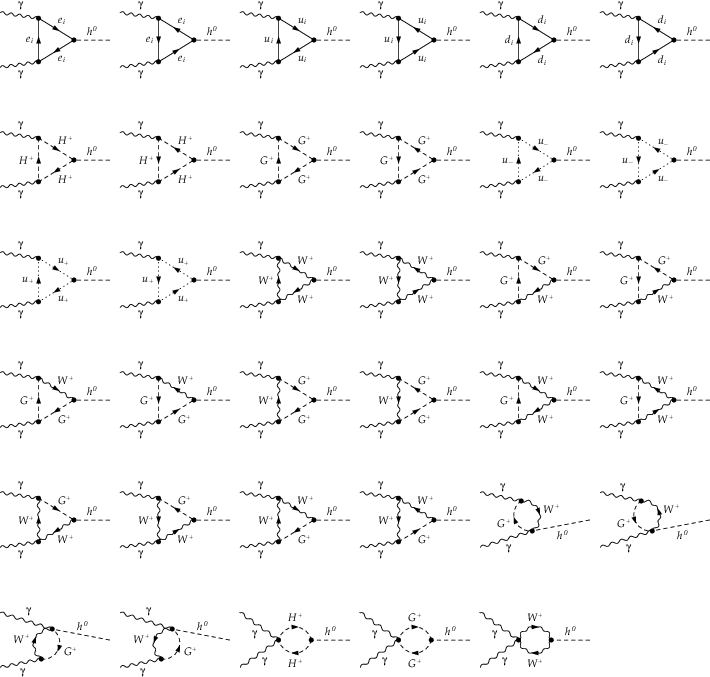
Although a tree-level -coupling is not allowed by the electromagnetic gauge symmetry, this interaction is generated at the quantum level through a plethora of radiative corrections, whose description in terms of Feynman diagrams is displayed in Figure 2. The entire set of diagrams corresponds to the production process for both CP-even states , whereas for the production of the CP-odd one, , only the first line of diagrams is allowed (owing to C and CP-invariance).
The relevant cross-section can be written in terms of the partial width of the decay as follows:
| (5) |
with the helicities of the two colliding photons and where we have used a standard representation for the -distribution. Following the above strategy, and computing the diagrams contributing to the amplitude with the help of the computational packages FeynArts, FormCalc and LoopTools [26], we may finally arrive at the -induced single Higgs boson cross-section. In order to obtain more accurate results, a running value for the electromagnetic coupling constant has been used.
3 Single Higgs boson production in a collider
The basic collider operates mainly through the mechanism of Compton (back)scattering of laser photons off the linac beams [13]. In a nutshell: a photon from a laser pulse collides with a high energy electron (or positron) at a small angle; as a result, the electron recoils and one is left with a Compton-scattered photon traveling in the direction of the original incident electron. The efficiency of the “conversion” will depend on many factors, such as the energy of each of the beams, the properties of the laser as well as on several non-linear effects and subleading mechanisms which turn out to modulate the overall process. As a matter of fact, the entire procedure comes down to furnish a luminosity spectrum, for which several standard parameterizations are available. This spectrum is essential to compute the expected number of events (in our case the number of produced Higgs bosons of a particular neutral species ). To this end, the cross-section computed in the previous section must be appropriately folded with the normalized (dimensionless) photon densities provided by the given parameterizations. The total (unpolarized) cross-section, after “conversion” of the primary linac beam, can finally be engineered from the following recipe:
| (6) |
where the partonic cross-section is given by
| (7) |
with ( being the CM energy of the primary linac machine). In the above expression, stands for the (differential) photon luminosity distribution constructed out of the photon densities as follows:
| (8) |
Functions and (one per beam of given polarization) are taken, in our case, from the standard package CompAZ [27].
In order to proceed with the numerical analysis, let us first of all examine the structure of the partonic cross-section. At fixed , it can be expressed from Eq. (5) in a simply manner:
| (9) |
If averaged over polarizations, the cross-section is given by the previous result but without the factor , because one has to sum over and divide by . For polarized photon beams of equal polarization (i.e. or ), the resulting cross-section is a factor of 2 larger. If, alternatively, we consider the case of opposite polarizations (), the cross-section vanishes (as expected from angular momentum conservation).
Let us emphasize that the partonic cross-section encodes already the relevant information regarding the dynamical features of the 2HDM under study. This information is obviously contained in the reduced amplitude of the effective vertex, and thus also in the branching ratio of . Notice that, in the region where the triple interaction dominates, the amplitude behaves roughly as . Obviously, in this region, the cross-section (9) is directly sensitive to the trilinear Higgs self-interaction (cf. e.g. the first two diagrams of the second row in Fig. 2), given by
| (10) | |||||
It follows from this expression that such coupling can be enhanced either at low or high values of , and also through the Higgs boson mass splittings – unlike the MSSM case. In addition, it may be heightened through its explicit dependence on the parameter 22 2 We note that for , Eq. (10) reduces to the corresponding result of Table 1 of Ref. [11], as it should. . Needless to say, in all cases these enhancements are strictly harnessed by the various theoretical and phenomenological constraints discussed in the previous section. By comparison, the corresponding (approximate) behavior of the amplitude for the SM contribution, if we assume that is dominated by the top quark Yukawa coupling, reads . This amplitude receives in general sizeable contributions from the gauge boson loops that significantly correct it. Similarly, in the domains of the 2HDM parameter space where the 3H-coupling (10) is not overwhelming over the Yukawa and gauge boson couplings (cf. e.g. the first, third and subsequent rows of diagrams in Fig. 2), our estimate above does not even hold as a crude approximation. Therefore, in general it is necessary to come to grips with the full expression for the effective coupling (which is indeed the main object under study, mainly for the cases ). Even more useful is to define the exact ratio between the corresponding 2HDM and SM coupling strengths at one-loop:
| (11) |
Obviously, the 2HDM amplitude will depend on whether the model is of type-I or type-II. In the particular region where the trilinear coupling dominates for production, the expectation on that ratio is roughly of order . Therefore, in the regime of large , for which , we can foresee a big enhancement with respect to the SM. To be sure, in practice we will perform the numerical analysis of the exact expression (11) and consider its behavior in general regions of parameter space.
For the sake of convenience, let us focus hereafter on the sets of Higgs boson masses displayed in Table 1 below.
| 2HDM | Set I | Set II | Set III | Set IV |
|---|---|---|---|---|
The mass spectrum in Set I of Table 1, for instance, allows to enhance the coupling. Its maximum value is roughly attained for , and . Incidentally, notice that the aforementioned Set I of masses is only suitable for type-I 2HDM, due to the relatively light value chosen for the charged Higgs boson ( GeV), which is below the (indirect) limit of GeV afflicting the type-II models [20]. Let us recall that, experimentally, the current C.L. direct mass limits for general Higgs bosons searches are: GeV for the charged Higgs boson, and GeV, GeV () for the neutral ones (of course with ) [21].

In Fig. 3, we perform the numerical analysis of the averaged total cross-section , Eq. (6), in which the partonic contribution is folded with the effective luminosity function (8). We display as a function of the center-of-mass (CM) energy of the linac machine for the Set I of Higgs masses. In this figure, we explore a region of parameter space where the coupling dominates for different negative values of (As we will see later on, large values are forbidden by vacuum stability.). Notice that, for sufficiently large , the cross-sections can be considerably high (spanning the range pb) at the fiducial startup value GeV of the ILC, and entailing at this point more than events for the given integrated luminosity. The rates, however, decrease fast for smaller values of , the reason being the destructive interference between the charged Higgs, gauge boson and fermion loops at low values of . For example, at the same energy and for we obtain fb respectively. Clearly, there is a delicate balance in the low region which amounts to a severe depletion of the overall 2HDM cross-section. By comparison, the corresponding result in the SM, namely for the same Higgs mass (), reads fb (hence events at that energy and luminosity range), which is quite sizeable. It follows that even small departures from this value should be measurable, especially in a high precision instrument as a collider.

In Fig. 4, we test the dependence of the cross-section on the Higgs masses. Specifically, we plot its evolution in terms of (left panel) and (right panel). We take the other parameters from Set I while keeping , , and choose three different values for : , and . Included is also the SM cross-section . Worth noticing is the fact that, while the 3H coupling is dominant, the cross-section does not immediately drop with ; it actually increases for a while up to a few hundred GeV. Moreover, for large values of , the evolution of presents a notorious “spike-shaped” enhancement near GeV, which is brought about by the threshold effect of two real charged Higgs bosons in the loop. The corresponding effect for a pair of real vector bosons at GeV is also barely visible therein.
The sharp suppression dip standing out on the right panel of Fig. 4 deserves also a few words. Recall that, in the regime in which the influence of the trilinear contribution () greatly “waxes”, the charged-Higgs mediated correction holds absolute sway over the loop-induced coupling . However, as soon as we raise the charged Higgs mass, the positive influence of the trilinear Higgs boson interaction rapidly wanes and it cancels more and more against the (negative) effects from the gauge boson and fermion loops. This gives rise to the aforementioned destructive interference. Eventually, a particular value of is reached where the two sorts of effects virtually annihilate each other (right at the vertex of the dip in the figure). Beyond this point, one rapidly reaches a regime where only the gauge boson and Yukawa coupling (negative) effects remain. Most of this region is actually excluded by the constraints. The destructive interference pattern described here is only possible when the set of Higgs boson masses is relatively light, as in the case of Set I under consideration, otherwise the trilinear effects could not be competitive.
The behavior of the effective coupling in the 2HDM can be better assessed in terms of the ratio defined in (11). Its dependence on the Higgs mass spectrum is sampled in Table 2 using the parameter setups indicated in Table 1. Set II, for instance, contains a heavier neutral CP-even Higgs sector which results in a sizeable value of of . It means that, in this case, the effective strength of the vertex almost quadruples that of the SM (). This is quite remarkable. On the other hand, Sets III and IV are characterized by heavier charged Higgs bosons and at the same time by a heavier CP-odd Higgs bosons (so as to elude the bounds). Unsurprisingly, the ratio falls in this case to within values below , i.e. close to the SM from below. As it should be expected, the larger the charged Higgs mass is, the less efficient is the enhancement capabilities associated to the 3H self-interactions. Incidentally, let us notice that Sets III and IV of Higgs-boson masses are intended to describe type-II 2HDM. Does this mean that for type-II models (those closer to the MSSM Higgs sector) there is no hope to hint at non-SM Higgs boson physics with collisions? Not necessarily so, as there is a tail of subleading one-loop effects triggered by the non-SM Yukawa couplings of the 2HDM in combination with the gauge bosons; in particular, we have already detected it in Fig. 4b for Set I (although within the excluded region). But, in general, this tail is available and lies well within the allowed region for heavier sets of Higss boson masses, such as Sets III and IV. More on it below.
A brief comparison with the existing calculations of single Higgs boson production within the MSSM is in order [17, 18]. For example, in Ref. [18] the ratio between the decay widths of the MSSM Higgs boson and the SM Higgs boson into is computed at one-loop. This ratio corresponds to the square of defined in (11). They find that, in the most favorable regimes (viz. large mass-splitting and large mixing angle in the top squark sector), it can lead to values of up to . It follows that the most optimistic MSSM expectations on are markedly below the maximum enhancement capabilities of the 2HDM (). The reason for this is clear and it was already advanced in the introduction – namely, the 3H self-couplings within the MSSM are restricted to be gauge-like and cannot source the potentially large effects that we have identified within the general 2HDM. Therefore, what we have called the “tail of subleading effects” in the 2HDM case is actually one of the main sources of the MSSM effects, the other being the supersymmetric Yukawa couplings of the Higgs bosons with the squarks.
| Set I | Set II | Set III | Set IV | |
| 3.98 | 3.75 | 0.98 | 0.98 | |
| 1.7 | 1.7 | 1.0 | 1.0 | |
| -0.86 | -0.86 | -0.82 | -0.82 | |
| -25 | -25 | 0 | 0 |
Figure 5 presents the corresponding contour lines for the ratio (11) in the plane. The cross symbol indicated on the left at the bottom denotes the point in this plane where such ratio attains the maximum value permitted by all the constraints. Moreover, we show the regions excluded by vacuum stability and by unitarity of the trilinear and quartic Higgs boson couplings. Notice that the sign is mostly forbidden by vacuum stability, which explains why we have presented the numerical analysis of the previous figures only for . In any case, we see that there is a sizable region left where the effective 2HDM coupling is significantly larger (in fact, a few times larger) than the SM coupling .

Finally, the available domains across the plane wherein one can obtain enhanced values of the ratio with respect to the SM case is explored systematically in Fig. 6 for different values of and at the fiducial startup energy GeV of the ILC. Specifically, in this figure we compute those regions in which the predicted value of the ratio exceeds the corresponding SM value () by at least while still being compliant with the full set of constraints; equivalently, regions where the cross-section is augmented by or more, thus inducing an excess of about one thousand events above the SM prediction (within the given luminosity segment). As we can see, the projected domains are sizeable. Interestingly enough, even tiny departures of from would already be significant, as they would amount to events up or down the SM expectation. If we would adopt this softer criterion, the allowed domains in Fig. 6 would be substantially augmented.
Particularly stringent is the impact of the unitarity restrictions, which translates into a progressive shrinking of the relevant region as we raise the value of .

For completeness, we have also addressed the single production of a heavy CP-even and a CP-odd Higgs boson. Their respective maximum cross-sections (at GeV) for the specific case of Set I read as follows: and . The former is of the order of itself, whereas the latter is significantly smaller, the depletion being caused by the absence of trilinear couplings of with the charged Higgs bosons. Furthermore, we wish to emphasize the existence of a region of parameter space where and can both be simultaneously sizeable. That region (e.g. for Set I) is just the allowed domain in the down-right corner in Fig. 5. There we find pb and pb, entailing some events within the standard luminosity range. This possibility can be very relevant, as it could be responsible for a potentially distinctive 2HDM signature which is unmatched in the MSSM.
We have also tested the enhancement potential of the 2HDM in the domains of parameter space where the 3H-coupling (10) is not relevant and where the bulk of the contribution concentrates on the Higgs-fermion Yukawa couplings in combination with the gauge bosons. In the case of generic type-II models, there is no enhancement at large (unlike the supersymmetric case) inasmuch as is severely constrained by unitarity. In general, due to the destructive interference between the diagrams dominated by the 3H-coupling and the rest (fermion and gauge boson loops), the enhancement capabilities of the Yukawa sector become overshadowed. As a consequence, in such region we meet the following situation: 1) There are still non-negligible domains in the 2HDM parameter space where the cross-section departs remarkably from its SM counterpart. However, in most cases the departure entails a significant (e.g. ) reduction of the cross-section with respect to the SM; 2) type-I and type-II models become essentially indistinguishable in that domain. This is a reflect of the fact that the Higgs-top quark coupling (which has the same form in either type-I and type-II models) drives the leading contribution in the Yukawa sector, whereas the gauge boson contribution is common in both types of models. Therefore, spotting a tail of non-SM effects in this region could not distinguish the type of 2HDM. Still, the missing number of events could certainly hint at the existence of a smoking gun triggered by physics beyond the SM.
Let us close this section by briefly mentioning that we have also surveyed the impact of another, more restrictive, set of unitarity constraints [22]. We have found that, in the most optimistic scenario for production in collisions, the coupling lies roughly a factor below the largest value it can take under the current set of constraints (1) and (2). Correspondingly, the enhancement with respect to the SM would be a factor times milder, thus dwarfing the relevance of the main effects in some regions of the parameter space. We point out, though, that the unitarity restrictions proposed in [22] are not fully coincident with those considered in [23], and in this sense there is still some controversy in the literature on this issue.
4 Single Higgs boson production through fusion
The interest on virtual photon-fusion (“two-photon processes”) certainly has a long and widespread history in Particle Physics. For instance, a prospect for the measurement of the pion lifetime from
| (12) |
was first discussed by F. Low almost half a century ago [28]. Studies of these processes, as well as detailed considerations on two-photon production of muon pairs and multi-pion final states, were carried out subsequently in the seventies [29]. Remarkably enough, long after the first pioneering studies appeared, two-photon processes are still an active and fruitful field of investigation, in particular for Higgs boson production. In actual fact, single Higgs boson production is, in a sense, the modern counterpart of Low’s “single-meson” production from quasi-real two-photon collisions. Already in the early eighties, this Higgs production channel was first studied in the literature within the context of the old (pre-LEP) colliders by J.A. Grifols and R. Pascual [15].
To be sure, the traditional two-photon processes are the forerunner of the future colliders considered in the previous section. These colliders will probably concentrate most of the interest around linac physics in the future and may greatly supersede the former in all practical searches for new physics. It is instructive to see once more why, specially in regard to the “Higgs issue”, a most sensitive matter these days. To this end, we compute here the cross-section for the processes
| (13) |
and compare with the results for real collisions studied in the previous section. In practice, we concentrate on the lightest CP-even state. Noteworthy is the fact that the cross-section for the virtual -fusion processes, in contradistinction to the real collisions, grows with the CM energy up to very high values of . Generically, the behavior of in the asymptotic energy regime goes as , where is the threshold mass of the produced final state , and the number depends on the high energy behavior of . The logarithmic growth simply tracks the dynamical feature by which, for these processes, the virtual photons can be quasi-real and hence have their momenta well-below the CM energy of the process, which may satisfy – the rest of the energy being carried away by the concomitant lepton final states. Recently, the pairwise production of Higgs-bosons via weak gauge-boson fusion mechanism, was analyzed in Ref. [12] at the leading order . The process turned out to be instrumental for probing the 3H self-interactions. A complementary strategy along the same lines is offered by the -fusion process (13), in which the loop-induced vertex at order can be dominated by the 3H coupling.

The technical complications associated to two-photon processes of the kind (12)-(13) were tackled long ago in the literature (cf. [29] for a classical review). The physics is also well understood, it boils down to the well-known equivalent-photon or Weizsäcker-Williams approximation, by which the virtual photon emitted from the scattered electron appears near the mass shell. This feature allows to essentially trade the process of electro-production for a photo-production one with an appropriate photon spectrum. The so-called photon content of a given electron can be explicitly factorized and the production cross-section can be approximated in the following way:
| (14) |
where and .
Figure 7 presents the logarithmic evolution of the production cross-section as a function of the CM energy. We have used the mass Set I and the optimal parameters quoted in Table 2. Once the production threshold has been surpassed, the cross-section suddenly increases up to a value of about pb and becomes persistently sustained, with only a mild (logarithmic) evolution. Over this approximate plateau, it amounts to more than events for an integrated luminosity fb-1, therefore resulting in an enhancement of one order of magnitude with respect to the SM. Even more remarkable is the fact that, despite the fairly large value of the two-photon cross-section, it is still a factor of (at least) smaller than that of the corresponding real scattering processes, for the same values of the 2HDM parameters (cf. Fig 3). This should explain vividly and convincingly the outstanding superiority of the future colliders versus the ancient two-photon processes.
5 Conclusions
We have devoted this work to analyze the production of a single neutral Higgs boson, , within the two-Higgs-doublet model (2HDM) through the following complementary mechanisms: i) direct scattering of real photons in a collider; and ii) fusion of a virtual photon pair in a conventional two-photon process, . Both mechanisms are direct handles on the effective interaction, . This coupling is a pure quantum effect generated by a plethora of radiative corrections involving charged Higgs bosons, quarks and gauge bosons. Among the interactions in the loops, we have the 3H self-interactions, most remarkably in the case of production – which proves to be utterly dominant in certain regions of the 2HDM parameter space. We have systematically swept this space and identified those configurations for which the departure from the SM prediction is most remarkable, and we have done this in full compliance with the rigorous constraints dictated by perturbativity, unitarity and vacuum stability bounds, as well as by the EW precision data. The result is that, in the most favorable scenarios, the physical cross-section (i.e. the one convoluted with the backscattered luminosity function) can typically reach the level of . In other words, may rocket to values bigger than the expected SM yield (for similar values of the Higgs mass), which by itself should already be perfectly measurable: pb fb. Such notorious enhancement can be traced back to the behavior of the coupling, despite it is highly restrained by the overall constraints. By sticking to moderate , it is possible to licitly increase the rates by choosing relatively large (negative) values of the parameter . Moreover, in order to optimize this mechanism, the charged Higgs boson should be relatively light (say, below ) so that the associated quantum corrections are not severely hampered by the decoupling effects. It means that the -enhancements that we have encountered apply only for type-I 2HDM, because for this kind of models the mass of the charged Higgs boson is not constrained by . A similar conclusion ensues for the case of double Higgs production in collisions, but with lower cross-sections [14].
In the above conditions, the expected number of single Higgs boson events emerging from direct scattering, within the typical energy range of the ILC (), is of the order of per of integrated luminosity. Compared to the production rate of single Higgs bosons through the traditional virtual photon-pair fusion, (which performs at the level of , at most, for ), the real -collision mechanism is at least one order of magnitude more efficient.
On the experimental side, the prospects for Higgs boson detection in a -collider are deemed to be excellent. To start with, let us stress that the single Higgs-boson final state is to be produced essentially at rest. Therefore, for , the corresponding signatures should mostly be in the form of back-to-back, highly energetic, quark jets (, ). For , instead, signatures with two or four charged leptons in the final state (from and, specially, from ) should be really pristine. Furthermore, we have seen that, in some cases, the two channels and are simultaneously accessible and with similar rates. Needless to say, this could result in a double distinctive signature of new physics.
With enough statistics on these events, and upon analyzing the invariant mass distribution of the resulting jets of quarks and leptons, the measurement of some 2HDM Higgs boson(s) mass(es) should be attainable with fairly good accuracy, together with a precise determination of the effective couplings (typically for and/or ). If their strengths would happen to be vastly dominated by the triple Higgs boson self-interactions, the signature of non-standard Higgs boson physics would be crystal-clear, leading us to suspect it to be rooted in some generic type-I 2HDM. However, should we meet the juncture or , the underlying quantum effects would be largely insensitive to the type of model and a more detailed comparative study with the MSSM would be mandatory [30]. Even then, tiny deviations could hint at new physics. In this regard, it is important to emphasize that, given the high precision nature of a collider, gathering a small effect (positive or negative) should be sufficient to point at a smoking gun.
Acknowledgments JS is grateful to F. Mescia for useful discussions on the bounds on the charged Higgs boson mass from low energy physics. NB thanks an ESR position of the EU project RTN MRTN-CT-2006-035505 Heptools; DLV acknowledges the MEC FPU grant AP2006-00357. DLV and JS have been supported in part by MEC and FEDER under project FPA2007-66665 and by DURSI Generalitat de Catalunya under project 2005SGR00564. This work was partially supported by the Spanish Consolider-Ingenio 2010 program CPAN CSD2007-00042.
References
- [1] H.P Nilles, Phys. Rept. 110 (1984) 1; H.E. Haber, G.L. Kane, Phys. Rept. 117 (1985) 75.
- [2] J.F. Gunion, H.E. Haber, G.L. Kane and S. Dawson, The Higgs hunter’s guide, Addison-Wesley, Menlo-Park, 1990.
- [3] D. Garcia and J. Solà, Mod. Phys. Lett. A9, 211 (1994); P.H. Chankowski, A. Dabelstein, W. Hollik, W. M. Mosle, S. Pokorski, J. Rosiek, Nucl. Phys. B417 (1994) 101; D. Garcia, R. A. Jiménez and J. Solà, Phys. Lett. B347 (1995) 309; Phys. Lett. B347 (1995) 321.
- [4] J. A. Coarasa, D. Garcia, J. Guasch, R. A. Jiménez, J. Solà, Eur. Phys. J. C2, 373 (1998); Phys. Lett. B425 (1998) 329; R. A. Jiménez, J. Solà, Phys. Lett. B389 (1996) 53; J.A. Coarasa, R. A. Jiménez, J. Solà, Phys. Lett. B389 (1996) 312; J. Guasch, R.A. Jiménez and J. Solà, Phys. Lett. B360 (1995) 47.
- [5] S. Heinemeyer, Higgs Physics at the LHC: Some Theory Aspects, arXiv:0807.2514 [hep-ph]; A. Djouadi, The Higgs sector of supersymmetric theories and the implications for high-energy colliders, arXiv:0810.2439 [hep-ph]; A. Djouadi, R.M. Godbole, Ewsb at LHC, arXiv:0901.2030 [hep-ph]; A. Djouadi, Phys. Rept. 457 (2008) 1; Phys. Rept. 459 (2008) 1.
- [6] ILC Reference Design Report Volume 2: Physics at the ILC, arXiv:0709.1893 [hep-ph]; Physics interplay of the LHC and the ILC, (G. Weiglein et al.), Phys. Rept. 426 (2006) 47.
- [7] A. Djouadi, W. Kilian, M. Mühlleitner and P.M. Zerwas, Eur. Phys. J C10 (1999) 27. For tree-level double Higgs production processes, see e.g. the exhaustive overview by M. Mühlleitner, hep-ph/0008127.
- [8] A. Djouadi, H.E. Haber and P.M. Zerwas, Phys. Lett. B375 (1996) 203; A. Djouadi, V. Driesen, W. Hollik and J. Rosiek, Nucl. Phys. B491 (1997) 68.
- [9] P. Osland and P.N. Pandita, Phys. Rev. D59 (1998) 055013; D.J. Miller and S. Moretti, Eur. Phys. J C13 (2000) 459; F. Boudjema and A. Semenov, Phys. Rev. D66 (2002) 095007.
- [10] A. Arhrib, R. Benbrik, C.-W. Chiang, Phys. Rev. D77 (2008) 115013, arXiv:0802.0319; A. Arhrib, W. Hollik, S. Penaranda, M. Capdequi Peyranere, Phys. Lett. B579 (2004) 361.
- [11] G. Ferrera, J. Guasch, D. López-Val, J. Solà, Phys. Lett. B659 (2008) 297; arXiv:0801.3907.
- [12] R.N. Hodgkinson, D. López-Val, J. Solà, Phys. Lett. B673 (2009) 47.
- [13] See e.g. V. I. Telnov, Nucl. Phys. Proc. Supp. 184 (2008) 271; Acta Phys. Pol. B 37 (2006) 1049; A. de Roeck, Nucl. Phys. Proc. Supp. 179-180 (2008) 94-103; B. Badelek et al., Int. J. of Mod. Phys. A 19 (2004) 5097.
- [14] F. Cornet and W. Hollik, Phys. Lett. B669 (2008) 58; E. Asakawa, D. Harada, S. Kanemura, Y. Okada and K. Tsumura, Phys. Lett. B672 (2009) 354; arXiv:0902.2458 [hep-ph]; A. Arhrib, R. Benbrik, C.H. Chen, R. Santos, arXiv:0901.3380 [hep-ph]; L. J. Dixon, Y. Sofianatos, Phys. Rev. D79 (2008) 033002; R. Martínez, J.Alexis Rodríguez and D. Milanés, Phys. Rev. D72 (2005) 035017.
- [15] J.A. Grifols, R. Pascual, Z. Phys. C6 (1980) 353.
- [16] G.V. Jikia, Nucl. Phys. B412 (1994) 57; R. Belusevic, G. Jikia, Phys. Rev. D70 (2004) 073017.
- [17] B. Grzadkowski, J.F. Gunion, Phys. Lett. B294 (1992) 361; J. F. Gunion, H.E. Haber, Phys. Rev. D48 (1993) 5; D.L. Borden, D.A. Bauer, D.O. Caldwell, Phys. Rev. D48 (1993) 4018; M. Mühlleitner, M. Krämer, M. Spira, P. Zerwas, Phys. Lett. B508 (2001) 311; D. M. Asner, J. B. Gronberg, J.F. Gunion, Phys. Rev. D67 (2003) 035009; P. Niezurawski, A.F. Zarnecki and M. Krawczyk, Acta Phys. Polon. B 37 (2006) 1187.
- [18] New results for a photon-photon collider, D. Asner, B. Grzadkowski, J. F. Gunion, H. E. Logan, V. Martin, M. Schmitt, M.M. Velasco, hep-ph/0208219; Photon photon and electron photon physics or physics at photon collider, M. Krawczyk, hep-ph/0307314.
- [19] A.W El Kaffas, P. Osland, Phys. Rev. D76 (2007) 095001.
- [20] M. Misiak et al. Phys. Rev. Lett. 98 (2007) 022002.
- [21] Particle Data Group (C. Amsler et al.), Phys. Lett. B667 (2008) 1.
- [22] S. Kanemura, T. Kubota and E. Takasugi, Phys. Lett. B313 (1993) 155; A. G. Akeroyd, A. Arhrib and E.-M. Naimi, Phys. Lett. B490 (2000) 119.
- [23] J. Horejsi and M. Kladiva, Eur. Phys. J C46 (2006) 81.
- [24] B.W. Lee, C. Quigg, H.B. Thacker, Phys. Rev. Lett. 38 (1977) 883; Phys. Rev. D16 (1977) 1519.
- [25] S. Kanemura, T. Kasai and Y. Okada, Phys. Lett. B471 (1999) 182.
- [26] T. Hahn, FeynArts 3.2, FormCalc and LoopTools user’s guides, available from http://www.feynarts.de; T. Hahn, Comput. Phys. Commun. 168 (2005) 78.
- [27] V. I. Telnov, Acta Phys. Polon. B 37 (2006) 633; A. F. Zarnecki, Acta Phys. Polon. B34 (2003) 2741.
- [28] F. Low, Phys. Rept. 120 (1960) 582.
- [29] H. Terazawa, Rev. Mod. Phys. 45 (1973) 615.
- [30] N. Bernal, D. López-Val, J. Solà, work in progress.