Planar electric trap for neutral particles
Abstract
A new geometry to trap neutral particles with an ac electric field using a simple electrodes structure is described. In this geometry, all electrodes are placed on a single chip plane, while particles are levitated above the chip. This provides an easy construction of the trap and a good optical access to the trap.
particle storage, atom optics, laser cooling
1 Introduction
To investigate the properties of particles such as atoms and molecules, it is desirable to hold them in an isolated environment. For this purpose, various kinds of traps have been developed. Among them, magneto-optical trap (MOT) and magnetic trap (MT) are successfully used for a variety of applications [1]. However they require the particles to have either a closed transition (MOT) or a magnetic moment (MT), which restrict the range of particles to be trapped. Electric trap (i.e. a trap that uses electric field), on the other hand, has the advantage that it can trap almost any kind of neutral particles. It is easily shown that it is impossible to trap neutral particles using a static electric field[2], and an ac electric trap was proposed to overcome this difficulty. [3, 4, 5] Disadvantage of such electric trap is its shallow trap depth (potential depth for sodium atoms is 190K for an electric field of 1kV mm-1), and one needs to make a small trap to increase the curvature of the potential and hold particles against the gravity. However ac electric traps proposed so far had solid structures and the fabrication of a small trap was rather difficult. For such technical reasons, ac electric traps were not realized until recently. [6, 7, 8, 9]
In this paper, we propose a new geometry of an ac electric trap in which all electrodes are placed on a single plane, while particles are trapped above that plane. Such geometry enables one to fabricate the trap structure in mass with high precision, which opens the possibility of making micro-structured atom and molecule chips that benefit from the advantages of long decoherence time [10], low electric power consumption, and scalability of the electric traps.
2 Principle of the dynamical trapping
We start from the trap configuration described in [[5]], schematically shown in fig. 1, in which all electrodes sit on a single plane (-plane). Two pairs of electrodes are placed on - and -axis symmetrically (i.e. at and ). There are two phases in the operation of this trap: In phase A (phase B) a voltage is applied on the pair of electrodes on -axis (-axis).

The potential that a neutral particle feels under the electric field is
| (1) |
where is the polarizability of the particle. is always positive for atoms or molecules in a stable state. In phase A or B, the potential has the form
| (2) |
up to 2nd order in . Here, is the mass of the particle and is the angular frequency of oscillation in -direction in phase A (-direction in phase B). For spherical electrodes and .[11] By switching between phase A and B alternatively for time and (usually ), particles are trapped around the origin : They are dynamically captured in -plane (similar to the RF ion trap[12]), whereas the confinement in -direction is static. Larger gives stronger confinement in -direction, while the stable region for the driving frequency is reduced with increasing ( is the period of the applied voltage).
3 How to lift up the trap point from the chip plane
Particles are trapped at the saddle point of . In order to lift up this trapping point off the -plane, we place additional electrodes in between the existing electrodes to bend the field lines and make a saddle point other than the origin (fig. 2). We still keep the electrodes configuration symmetric under , , . Now (2) becomes
| (3) |
near the new saddle point . Let be the scalar potential. In phase A (and similarily in phase B), because of , ,
| (4) |
so that . And also from and . From these equalities, , and thus is still satisfied.


3.1 Design procedure: step 1
First, we consider electrodes as point charges and place them on -plane as shown in fig. 3.


Four outer point charges placed at correspond to the four electrodes of the original configuration (fig.1) and we put charges of or 0 at appropriate phase. Four inner point charges at are added to the original configuration with charges depending on the phase (see figure). In fig. 4 we plot parameters , , that appear in (3) as functions of for several values ( is calculated from as ). Here is for the original configuration, i.e. .
(a)
(b)
(c)
Normalized potential is plotted along -axis for different in fig. 5, for different in fig. 6, and along - (-) direction in fig. 7.


We choose and to proceed the design procedure further. Relevant parameters for and are compared with those for the original configuration in table 1 (see section 5 for ).
| 0.06 | 0.34 | 0.85 | 1.94 | 0.94 | 0.64 |
|---|---|---|---|---|---|
| (0.0) | (0.0) | (1.0) | (2.0) | (1.0) | (1.0) |
3.2 Design procedure: step 2
Now we are going to replace the point charges by electrodes of finite size. For that, first we calculate the equipotential surface of the electric field. Figure 8a is the plot of the normalized scalar potential in the chip plane ().
(a)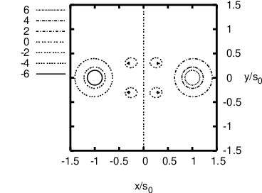 (b)
(b)
Equipotential surfaces of around the outer point charges at are nearly spherical for large and small , and can be well imitated by a disc shaped electrodes of radius centered at . However smaller gives higher electric field assuming that the voltage applied on the electrodes is fixed. In fig. 8b we choose (). We apply to these outer electrodes voltage of or 0 at appropriate phase: (i.e. ). Equipotential surfaces of around the inner point charges at are again nearly spherical for , and the inner point charges can be replaced by disc shaped electrodes of radius ( for , ) centered at which are always connected to the ground (0 voltage).
4 Trapping particles under the gravity of the earth
In this section, we give some practical values to trap neutral atoms and dielectric spheres on the earth. We orient -axis along the gravity direction. We set a condition that the gravitational sag should be smaller than (with ): . This gives . On the other hand . We fix here the trap design as , and which gives , . We also put and .
First we discuss on trapping neutral atoms. We choose sodium atoms as an example: , [13] kg, and thus . If we set mm, then the condition on the gravitational sag requires Hz. This will be satisfied with the applied voltage of V. Setting V, then Hz and, using fig. 12, the trap should be stable for ms with .
Next we discuss on trapping of a dielectric material. The polarizability of a dielectric sphere of radius and dielectric constant is (mass is where is the density) so that is independent of its size. Polystyrene(, ), for example, has the value , which is roughly one order smaller than that of sodium atoms.
5 Trapping of polar particles
In the case of polar particles of permanent dipole moment , the force under the electric field can be written as, assuming the direction of the dipole moment is always oriented parallel to the electric field (see appendix C),
| (5) |
Thus the force is derived from the potential
| (6) |
Near the trap center , , so that the dynamics of the polar particles can be argued in the same way as that of the nonpolar particles by replacing with . We define a dimensionless parameter where . Now . A plot of is given in fig.9.

For a particle of bulk material of permanent polarization and density , so that is independent of its shape and size. To give practical parameters, we again use the trap design , , and , and consider trapping of micro particles ( and ). If we set mm, then the condition on the gravitational sag with requires Hz which implies V. At V, Hz and, from fig. 12, the trap should be stable for ms.
6 Conclusions and outlook
We have presented a new design of ac electric trap for neutral particles and have shown that it is possible to make a trapping point above the chip surface with planar electrodes structure. We have also discussed about the feasibility of this design by showing typical parameters for trapping neutral atoms, dielectric spheres, and polar particles. The parameters for this trap were comparable with those demonstrated in [[6]]. In the final step of the design, we have used disc shaped electrodes to imitate the equipotential surface of the electric field. [14] To analyse its consequence, we are now calculating the electric field using numerical methods. The result is still preliminary, but it has turned out that the field near the trapping point is not so much dependent on the shape of the inner electrodes. Thus, as an application of our trap, a particle conveyor such as shown in fig. 10 should be also possible.

acknowledgement
This work was partly supported by the 21st Century COE
program of the University of Electro-Communications on
”Coherent Optical Science” supported by the Ministry of
Education, Culture, Sports, Science and Technology.
Appendix A Stability
In this section, we investigate the stable condition of the dynamical confinement. The equations of motion are separated in -, -, -directions so that we explore the motion in -direction only. We follow the procedure described in [[4]] and define a state vector as
| (7) |
where () is the position (velocity) of the particle at time t. Time evolution of is described by a time evolution matrix : .
| (8) |
with ( is the unit matrix).

We assume that the phase A starts at (fig. 11) so that with where () is the time evolution matrix for the phase ().
| (9) |
| (10) |
with . Let be the eigenvalue of .
| (11) |
with . From (11)
| (12) |
The trap is stable if and only if .

In fig. 12 we plot as a function of and () to show the stable region.
A.1 Unharmonicity
So far we have not included the unharmonic terms in the potential. In the original Stark chip configuration, the lowest unharmonic term was 4th order because of the symmetry. In our configuration, due to the absence of this symmetry, 3rd order terms are present. However these terms have the form
| (13) |
and are still harmonic in the plane (i.e. the plane in which the confinement is dynamical), we expect that the 3rd order terms do not reduce the stable region in phase space drastically.
Appendix B Trap tightness
To estimate the tightness of the dynamical confinement, we apply a constant force in -direction on the particle in the trap and calculate the shift of the trap center (i.e. the time average of the position of the particle). Let be the state vector at time with the initial condition . Then the time evolution of a general state vector is now .
| (14) |
| (15) |
| (16) |
To evaluate the time average of , we put with and , and take the average over and . Because inside the stable region, we obtain
| (17) |
After a lengthy calculation, (17) yields
| (18) |
and , where . In the limit , as expected. The effective trap frequency is calculated as . In fig. 13 we plot for as a function of and .

From this, we see that is obtained for .
Appendix C Dynamics of the polarization orientation of a polar particle
Consider a polar particle of size and volume () that consists from a bulk material under the electric field . Let be the angle between the electric field and the polarization of the material. Then
| (19) |
where is the moment of inertia and is the torque. where is density of the material ( for a sphere of diameter ). Assuming is small, (sphere: ). Angular frequency of oscillation of the polarization direction is thus (sphere: ). If the switching time between phase A and B is longer than , then the direction of the polarization adiabatically follows that of the electric field. For (see section 5) with m and , (sphere: ).
References
- [1] H. J. Metcalf and P. van der Straten: Laser Cooling and Trapping (Springer, New York, 1999).
- [2] W. Ketterle and D. E. Pritchard: Appl. Phys. B 54 403 (1992).
- [3] F. Shimizu and M. Morinaga: Jpn. J. Appl. Phys. 31 L1721 (1992).
- [4] M. Morinaga and F. Shimizu: Laser Phys. 4 412 (1994).
- [5] H. Katori and T. Akatsuka: Jpn. J. Appl. Phys. 43 358 (2004).
- [6] T. Kishimoto, H. Hachisu, J. Fujiki, K. Nagato, M. Yasuda, and H. Katori: Phys. Rev. Lett. 96 123001 (2006).
- [7] T. Rieger, P. Windpassinger, S. A. Rangwala, G. Rempe, and P. W. H. Pinkse: Phys. Rev. Lett. 99 063001 (2007).
- [8] S. Schlunk, A. Marian, P. Geng, A. P. Mosk, G. Meijer, and W. Schöllkopf: Phys. Rev. Lett. 98 223002 (2007).
- [9] H. L. Bethlem, J. van Veldhoven, M Schnell, and G. Meijer: Phys. Rev. A 74 063403 (2006).
- [10] In the case of an electric trap (as opposed to MT), the electrodes can be made thinner than the skin depth, which reduces the decoherence of atoms trapped in the vicinity of electrodes. See, C. Henkel and M. Wilkens: Europhys. Lett. 47 414 (1999).
- [11] Generally, from , we obtain inequality .
- [12] W. Paul and H. Steinwedel: Z. Naturforsch. A 8 448 (1953).
- [13] C. R. Ekstrom, J. Schmiedmayer, M. S. Chapman, T. D. Hammond, and D. E. Pritchard: Phys. Rev. A 51 3883 (1995).
- [14] The presence of the chip substrate on which electrodes are placed does not affect the electric field in the free space side as far as electrodes are thin and the substrate is thick compared to the electrodes structure.