Tidal alignments as a contaminant of redshift space distortions

If galaxies were randomly oriented, Eq. (6) would fully describe the linear regime. However, some classes of real galaxies, including LRGs, exhibit correlations of their orientation with large-scale structure (e.g. Binggeli 1982; see Hirata et al. 2007 for a recent measurement of the correlation function). This section defines the notation needed to handle selection effects that depend on galaxy orientation and viewing direction.

The galaxy orientation is described by 3 Euler angles $(\theta,\phi,\psi)$. These define a rotation matrix ${\textbf{{Q}}}(\theta,\phi,\psi)\in$SO(3) that transforms the “lab” frame coordinates to a frame aligned with the galaxy; see Appendix D for explicit expressions. The well-known volume element of SO(3) is

and its total volume is $\int_{\rm SO(3)}{\rm d}^{3}{\textbf{{Q}}}=8\pi^{2}$. We consider the conditional probability distribution ${\cal P}({\textbf{{Q}}}|{\mn@boldsymbol{x}})$ for the orientation Q of a galaxy at position ${\mn@boldsymbol{x}}$. In the case of randomly oriented galaxies we have ${\cal P}({\textbf{{Q}}}|{\mn@boldsymbol{x}})=1/(8\pi^{2})$, but in general this probability distribution may depend on the local environment (tidal field, density, etc.) at ${\mn@boldsymbol{x}}$.

Our next ingredient is the dependence of the observational selection function on the viewing geometry and galaxy orientation. We assume that the observer is looking along the line of sight²² 2 We define this so that the observer points their telescope in direction $\hat{\mn@boldsymbol{n}}$; the light from the galaxy is propagating in direction $-\hat{\mn@boldsymbol{n}}$. $\hat{\mn@boldsymbol{n}}$. The appearance of the galaxy then depends on the observer’s line-of-sight expressed in the galaxy frame, i.e. $\hat{\mn@boldsymbol{m}}={\textbf{{Q}}}\hat{\mn@boldsymbol{n}}$. It is therefore possible for the probability of selecting a galaxy to vary depending on ${\textbf{{Q}}}\hat{\mn@boldsymbol{n}}$:

We may take the anisotropy of the selection function to have mean zero when averaged over all possible viewing directions,

since any ${\hat{\mn@boldsymbol{m}}}$-independent constant added to $\Upsilon$ can be absorbed into the local galaxy density. Note that Eq. (10) implies that the selection probability variation averaged over all possible orientations is also zero, i.e.

The tidal alignment effect on large scale structure observations depends on the combination of the intrinsic alignment model, which determines ${\cal P}({\textbf{{Q}}}|{\mn@boldsymbol{x}})$, and the dependence $\Upsilon$ of the selection function on geometry. The number density of selected galaxies $N({\rm selected})$ is then related to the true number density of galaxies $N({\rm true})$ by averaging Eq. (9) over the distribution of galaxy orientations at ${\mn@boldsymbol{x}}$:

This motivates defining

which represents the viewing direction dependent selection function at position ${\mn@boldsymbol{x}}$. Examining Eq. (11), we see that $\epsilon$ vanishes if either the galaxy orientations are isotropically distributed [in which case ${\cal P}({\textbf{{Q}}}|{\mathbf{x}})=1/(8\pi^{2})$], or if $\Upsilon$ vanishes. Both intrinsic alignments (${\cal P}$ depends on Q) and orientation-dependent selection ($\Upsilon\neq 0$) are required to produce an effect on large scale structure.

[In the case of an axisymmetric disk galaxy, the third Euler angle $\psi$ is irrelevant. In this case, integrals such as Eq. (13) reduce to integrals over the disk normal vector $\hat{\mn@boldsymbol{L}}$.]

The real-space density of observed galaxies at position ${\mn@boldsymbol{x}}$ as seen by an observer looking in direction $\hat{\mn@boldsymbol{n}}$ has fluctuation

In a real galaxy survey, the actual viewing direction $\hat{\mn@boldsymbol{n}}$ is $\hat{\mn@boldsymbol{e}}_{3}$, and our final computation of the galaxy properties will be obtained by substituting $\hat{\mn@boldsymbol{n}}=\hat{\mn@boldsymbol{e}}_{3}$ into Eq. (14).

Equation (10) implies that $\epsilon(\hat{\mn@boldsymbol{n}}|{\mn@boldsymbol{x}})$ to average to zero over the unit sphere (i.e. over all possible viewing directions),

We then find, instead of Eq. (5), the observed redshift-space galaxy density in the linear regime is

In order to construct the observed galaxy power spectrum, we need to develop the statistics of $\epsilon(\hat{\mn@boldsymbol{n}}|{\mn@boldsymbol{x}})$. This is a random field as a function of a position ${\mn@boldsymbol{x}}$ and direction $\hat{\mn@boldsymbol{n}}$, and its statistical description can be achieved in the same way that one decomposes the CMB temperature $\delta T({\mn@boldsymbol{x}},\hat{\mn@boldsymbol{n}})$ in cosmological perturbation theory (Ma & Bertschinger, 1995; Hu & White, 1997). One first Fourier transforms the spatial variables to get $\tilde{\epsilon}(\hat{\mn@boldsymbol{n}}|{\mn@boldsymbol{k}})$. Then one introduces a rotation matrix ${\textbf{{R}}}\in$SO$(3)$ that rotates the unit vector $\hat{\mn@boldsymbol{k}}$ to the $\hat{\mn@boldsymbol{e}}_{3}$ axis, i.e. ${\textbf{{R}}}\hat{\mn@boldsymbol{k}}=\hat{\mn@boldsymbol{e}}_{3}$.³³ 3 Note that R is not unique, since it amounts to an arbitrary choice of which unit vector in the plane orthogonal to ${\mn@boldsymbol{k}}$ gets rotated to $\hat{\mn@boldsymbol{e}}_{1}$. Here R depends on $\hat{\mn@boldsymbol{k}}$, but we will not write this dependence explicitly to avoid confusion. Finally, we decompose the dependence of $\tilde{\epsilon}(\hat{\mn@boldsymbol{n}}|{\mn@boldsymbol{k}})$ on the viewing direction $\hat{\mn@boldsymbol{n}}$ into spherical harmonics,

This corresponds to choosing the “North Pole” of the spherical harmonic basis to be in the direction $\hat{\mn@boldsymbol{k}}$. We note that Eq. (15) eliminates the $l=0$ term.

Translation invariance forces different ${\mn@boldsymbol{k}}$-modes to be independent, and rotational invariance around ${\mn@boldsymbol{k}}$ forces different different values of $m$ to be independent. Therefore, we can write the power spectrum of $\epsilon$:

These power spectra are not arbitrary. Appendix A shows that since $\epsilon(\hat{\mn@boldsymbol{n}}|{\mn@boldsymbol{x}})$ is a real field, $P_{\epsilon}^{ll^{\prime}m}(k)$ must also be real. Invariance under reflection across a plane containing ${\mn@boldsymbol{k}}$ forces the restriction

and by swapping the $l$ and $l^{\prime}$ labels in Eq. (18) and recalling that the power spectra are real, we find the symmetry relation:

Therefore the power spectra are completely described by the cases with $0\leq m\leq l^{\prime}\leq l$, with $l,l^{\prime}>0$.

In addition to its intrinsic power spectrum, $\epsilon$ can have a cross-power spectrum with the matter field. This can be defined in analogy to Eq. (18). The matter field has the same symmetry as the $l=m=0$ mode of $\epsilon$ (if it existed), so by rotational symmetry only the $m=0$ components of $\epsilon$ can correlate with the matter field. We thus have

for $l>0$. Again, $P_{{\rm m}\epsilon}^{l}(k)$ must be real.

A further simplification is possible for galaxies that are inversion-symmetric, i.e. have the same appearance if viewed from the opposite direction. This is true for optically thin, triaxial elliptical galaxies, and is true for disk galaxy models that are axisymmetric and have a reflection symmetry across their equatorial plane. It may also be true in a statistical sense for real disk galaxies: while the specific arrangement of dust and H ii regions will not have inversion symmetry, it is plausible that these local imperfections would be unique to each galaxy and not correlated with large-scale structure. In this case, $\epsilon(\hat{\mn@boldsymbol{n}}|{\mn@boldsymbol{x}})=\epsilon(-\hat{\mn@boldsymbol{n}}|{\mn@boldsymbol{x}})$ and hence $\tilde{\epsilon}_{lm}({\mn@boldsymbol{k}})=0$ for odd $l$. All power spectra with odd $l$ or $l^{\prime}$ then vanish.

In traditional cosmology language, the $m=0$ contributions to this equation are scalars, $m=\pm 1$ are vectors, $m=\pm 2$ are tensors, and so on. One would expect in the linear regime that only the scalars ($m=0$) are present since large-scale density perturbations are scalars and cannot source any alignment of galaxies with $m\neq 0$ symmetry. (Physically, in the absence of mode coupling, a Fourier mode ${\mn@boldsymbol{k}}$ possesses rotational symmetry around the axis $\hat{\mn@boldsymbol{k}}$ that prevents any $m\neq 0$ component.) At small scales it is possible that the $m\neq 0$ alignments arise from nonlinear mode coupling. Since Eq. (16) is valid only when the density and velocity fields are in the linear regime, in the body of this paper we will only consider the scalar ($m=0$) intrinsic alignments. We note, however, that the scale at which nonlinear effects start to influence intrinsic alignments is unknown and may be larger than the traditional $k_{\rm max}^{-1}\sim 10h^{-1}$ Mpc used in galaxy surveys. In this case one might want the equations describing a general intrinsic alignment model; these are given in Appendix B.

Having defined the intrinsic alignment power spectra, we now compute the observed redshift-space power spectrum of the galaxies, i.e. of Eq. (16). We consider here only scalar intrinsic alignments with even $l$ only (i.e. we assume inversion symmetry). We first plug in Eq. (17),

Taking the power spectrum gives

Here the first term is the conventional redshift-space power spectrum, the second comes from correlations of the matter (and velocity) fields with intrinsic alignments, and the final term is the pure intrinsic alignment term.

Equation (23) can be simplified by replacing $Y_{l0}$ with a Legendre polynomial.⁴⁴ 4 Following convention, we denote the Legendre polynomials by $P_{l}$ and associated Legendre polynomials by $P_{l}^{m}$. By context these should not be confused with power spectra. We can evaluate its argument via

where the first equality is the definition of $\mu$, the second is the definition of a rotation matrix, and the third follows from the condition ${\textbf{{R}}}\hat{\mn@boldsymbol{k}}=\hat{\mn@boldsymbol{e}}_{3}$. Thus

This substitution gives rise to

We model an elliptical galaxy as an optically thin (i.e. negligible dust) triaxial system. The volume emissivity at a position ${\mn@boldsymbol{s}}$ relative to the centre of the galaxy is taken to be $j({{\mn@boldsymbol{s}}})={\cal J}(\rho)$, where the ellipsoidal radius $\rho$ is $\rho^{2}={\mn@boldsymbol{s}}\cdot{\textbf{{V}}}^{-1}{\mn@boldsymbol{s}}$. The matrix V is symmetric and unimodular ($\det{\textbf{{V}}}=1$) and contains information about the anisotropy of the galaxy, whereas ${\cal J}(\rho)$ specifies the radial profile. For a spherical galaxy, ${\textbf{{V}}}={\textbf{{I}}}$. We define the deviation from spherical symmetry to be ${\textbf{{W}}}\equiv{\textbf{{V}}}-{\textbf{{I}}}$, and will work in the limit where W is small. To first order, W is traceless. It is described by 5 numbers: 2 linearly independent eigenvalues that specify the amount and type (oblate vs. prolate) of triaxiality, and 3 Euler angles. We will argue here that for small W, the selection probability $\Upsilon({\textbf{{Q}}}\hat{\mn@boldsymbol{e}}_{3},{\mn@boldsymbol{x}})$ is proportional to $W_{33}({\mn@boldsymbol{x}})$. Then in accordance with Eq. (13) we will find that $\epsilon(\hat{\mn@boldsymbol{e}}_{3}|{\mn@boldsymbol{x}})\propto\langle W_{33}\rangle({\mn@boldsymbol{x}})$, where the coefficient of proportionality depends on the selection algorithm. We will argue that $\langle W_{ij}\rangle({\mn@boldsymbol{x}})\propto s_{ij}({\mn@boldsymbol{x}})$ (see Appendix D for an explicit demonstration in terms of the integral over Q). The coefficient of proportionality, needed to determine $A$, will be fixed using measurements of galaxy ellipticity-density correlations.

We do not observe the full 3-dimensional structure of the galaxy, but rather its 2-dimensional projection

where ${\mn@boldsymbol{s}}_{\perp}$ is a position in the plane of the sky, i.e. the 12-plane.

In Appendix C, we show that the observed two-dimensional projection is

Here

is the projected image of the spherical galaxy model,

is a rescaled skewer position in the 12-plane, and ${\textbf{{W}}}_{\perp}$ is the projection of W into the 12-plane (i.e. the $2\times 2$ submatrix). Note that ${\textbf{{W}}}_{\perp}$ need not be traceless; indeed Tr$\,{\textbf{{W}}}_{\perp}=-W_{33}$.

The observed properties of this galaxy are as follows. The effective radius $r_{\rm e}$ is reduced from its spherical version in accordance with Eq. (39):

The total flux $F$ of the galaxy is unchanged. Finally, the ellipticities of the isophotes (surfaces of constant $c$) components are

LRGs are usually selected by a combination of cuts in colour space, combined with a magnitude cut. As long as the galaxy is optically thin, there is likely to be very little orientation-dependent change in colour. However, the apparent magnitude of a galaxy may depend strongly on its orientation. Here we provide some examples.

Model magnitudes: If galaxies are selected based on model magnitudes, and the model fit accurately describes the radial profile, then the model-fit magnitude corresponds to the orientation-independent flux $F$. This gives $\epsilon=0$.

Petrosian magnitudes: For galaxies described by a single radial profile ${\cal J}(\rho)$ (e.g. a deprojected de Vaucouleurs model), that are well-resolved (in the sense that the Petrosian radius is well beyond the smearing of the central cusp due to the point-spread function), and have small ellipticity (W small), the Petrosian magnitude should be invariant under the rescaling of $r_{\rm e}$ described by Eq. (40). This is because the Petrosian radius will be a fixed multiple of $r_{\rm e}$ and will capture a fixed fraction of the galaxy’s flux. Within these approximations we would have $\epsilon=0$, but the robustness of this conclusion should be tested in simulations if high accuracy is required.

Aperture magnitudes: If galaxies are selected based on aperture magnitudes, then we count more of a galaxy’s light when it is viewed down a long axis than a short axis. As an example, suppose that the aperture is cut off at $y$ effective radii the spherical galaxy model, and the shape of the galaxy’s profile is such that the fraction of the luminosity within $yr_{\rm e}$ is ${\cal Q}(y)$. A 1 per cent decrease in $r_{\rm e}$ results in a 1 per cent increase in $y$ and hence a $y{\cal Q}^{\prime}(y)/{\cal Q}(y)$ per cent increase in ${\cal Q}(y)$. Then using Eq. (40), the aperture flux $F_{\rm ap}$ is modified according to

If the galaxies are selected according to a flux limit and the cumulative luminosity function of galaxies has logarithmic slope $\eta$, i.e. ${\rm d}\ln\bar{n}/{\rm d}\ln F_{\rm min}=-\eta$, then a 1 per cent increase in measured flux for galaxies near threshold corresponds to an $\eta$ per cent increase in the number density. Thus

Isophotal magnitudes: Isophotal magnitudes are similar to aperture magnitudes in that we count more of a galaxy’s light when it is viewed down a long axis than a short axis. However, in this case the cutoff for flux determination depends on the surface brightness profile. The surface brightness at $y$ effective radii is

If we change $r_{\rm e}$ but hold the surface brightness constant (as appropriate for determining how the isophotes move), we find

The quantity in brackets evaluates to ${\cal Q}^{\prime\prime}(y)/{\cal Q}^{\prime}(y)-y^{-1}$. We also know from Eq. (40) that $\delta r_{\rm e}/r_{\rm e}=-W_{33}/4$. Thus we may solve for $\delta y$:

This implies a fractional change in isophotal flux of

For a luminosity function slope $\eta$, we find

Note that the coefficient of $W_{33}$ is positive, because ${\cal Q}^{\prime\prime}(y)/{\cal Q}^{\prime}(y)-y^{-1}<0$ for any surface brightness profile that decreases as one moves outward (e.g. de Vaucouleurs).

In all of these cases, one may write

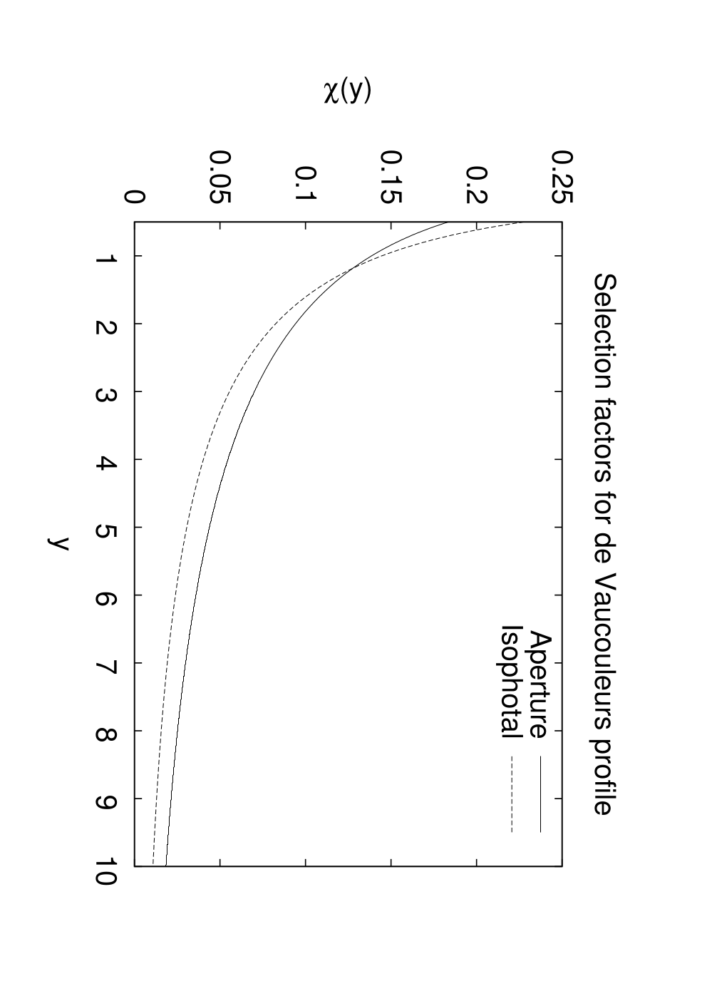
where $\chi$ depends on the method of computing fluxes (model, Petrosian, aperture, or isophotal), the galaxy profile, and (in the latter two cases) the typical number of effective radii $y$ at which the flux is computed for galaxies near the threshold. For the de Vaucouleurs (1948) profile, where ${\cal Q}^{\prime}(y)\propto y\exp(-7.67y^{1/4})$, values of $\chi$ are shown in Figure 2. Note, however, that Petrosian, aperture, or isophotal magnitudes of galaxies at radii affected by the point-spread function of the telescope would exhibit more complicated behavior that depends also on the dimensionless resolution factor (model magnitudes will be affected too if the model does not correctly describe the galaxy).

We now suppose that the mean value of W for galaxies in a particular region of space has some dependence on the tidal field surrounding it. Since both $W_{ij}$ and the tidal field $s_{ij}$ are traceless-symmetric tensors and have quadrupolar symmetry, the lowest-order allowed term in the Taylor expansion of $W_{ij}$ as a function of $s_{ij}$ is:

An alternative argument for Eq. (50) in terms of the Euler angles can be found in Appendix D. We also argue there that although the full specification of the alignment of a triaxial galaxy to linear order in $s_{ij}$ requires 2 parameters, the statistical effect on $\langle W_{ij}\rangle$ only involves 1 parameter ($B$).

Comparing Eq. (50) to Eqs. (28) and (49) gives the proportionality coefficient,

As discussed in Sec. 3.1, there is an effect on large scale structure only when the galaxies have nonrandom orientations ($B\neq 0$) and when there is an orientation-dependent selection effect ($\chi\neq 0$).

The normalization constant $B$ depends on the details of elliptical galaxy formation. Rather than choosing a value based on theoretical considerations, we normalize $B$ to measurements of intrinsic ellipticity correlations of elliptical galaxies. Using Eq. (41), we find that for a Fourier mode ${\mn@boldsymbol{k}}$ perpendicular to the line of sight, e.g. in the 1-direction (${\mn@boldsymbol{k}}=k\hat{\mn@boldsymbol{e}}_{1}$), we have $\tilde{e}_{1}({\mn@boldsymbol{k}})=B\tilde{\delta}_{\rm m}({\mn@boldsymbol{k}})$. This implies a cross-power spectrum between matter and ellipticity of

This power spectrum – or more precisely, the cross-correlation – was measured by Hirata et al. (2007), who were interested in intrinsic alignments as a contaminant of cosmic shear measurements. For the latter reason, Hirata et al. (2007) presented not the correlation with ellipticity components $e_{1,2}$ but with “intrinsic shear” $\gamma^{\rm I}_{1,2}\equiv e_{1,2}/1.74$, where 1.74 is the shear responsivity. Note that in the notation of Bernstein (2008), $b_{\kappa}=B/1.74$. The projected correlation function $w_{\delta+}(r_{\rm p})$ of the matter and intrinsic shear is

Hirata et al. (2007) showed that the scale dependence implied by Eq. (53) is a good fit to the intrinsic alignments of LRGs. They normalized their correlation function by its value at $r_{\rm p}=20h^{-1}\,$Mpc and $z=0.3$, and using the nonlinear matter power spectrum (Smith et al., 2003), Eq. (53) gives a correlation function of $-3.3b_{\kappa}h^{-1}\,$Mpc. Comparing to the observed value of $0.059(L/L_{0})^{1.48}h^{-1}\,$Mpc (where $L$ is the luminosity $K+e$-corrected to $z=0$ and $L_{0}$ corresponds to a corrected $r$-band absolute magnitude $M_{r}^{0.0}$ of $-22$) suggests that

Thus at $z=0.3$, $B\approx-0.03$ for LRGs of magnitude $M_{r}^{0.0}=-22$, rising to $-0.06$ at $M_{r}^{0.0}=-22.5$ and $-0.12$ at $M_{r}^{0.0}=-23$.

In order to estimate the anisotropic selection parameter $A$, we additionally need the slope of the cumulative luminosity function $\eta=-{\rm d}\ln\bar{n}/{\rm d}\ln F_{\rm min}$. We may use the LRG luminosity function of Wake et al. (2006).⁶⁶ 6 Wake et al. (2006) note that for typical LRGs, $M_{r}^{0.2}\approx M_{r}^{0.0}+0.11$; but note that the absolute magnitude in Hirata et al. (2007) is referenced to 10$h^{-1}$ pc, whereas Wake et al. (2006) refers absolute magnitudes to 10 pc assuming $h=0.7$. This introduces an additional offset of $5\log_{10}0.7$ so that the magnitudes in Wake et al. (2006) are given by $M_{r}^{\rm Wake}=M_{r}^{0.0}-0.66$. At $M_{r}^{0.0}=-22.5$, we find $\eta=4.0$. If galaxies are selected with isophotal magnitudes with a surface brightness cutoff at $\sim 3r_{\rm e}$, then $\chi\sim 0.05$. Combining with $B\sim-0.06$, this leads to $A\sim-0.024$. Since at $z=0.3$, $f\approx 0.65$, we find that the fractional contamination to the redshift-space distortion measurement $|A|/f$ is $\sim 4$ per cent. For LRGs a half a magnitude brighter at $M_{r}^{0.0}=-23$, $\eta=4.5$ and $B\sim-0.12$, so the contamination increases to $\sim 8$ per cent. If one used aperture magnitudes instead, with a typical aperture cutoff at $\sim 3r_{\rm e}$, then we would have $\chi\sim 0.06$ and our estimated fractional contamination $|A|/f$ for these two cases would rise to 5 and 10 per cent, respectively.

These values are extremely rough and are merely intended to show that there exist regimes in which the cosmological interpretation of the redshift-space distortions is significantly altered. The level of contamination for a particular survey depends in great detail on its selection criteria; if it is significant, $\eta\chi$ would best be determined by a combination of Monte Carlo simulations and direct use of the observed distribution of galaxies in colour-magnitude space rather than the simplified analytic arguments used here. Also note the sign: for isophotal or aperture magnitude selection, where galaxies are more likely to pass cuts if aligned in the radial direction, we have $A<0$.

The leading spectroscopic LRG surveys today, such as the SDSS LRG survey (Eisenstein et al., 2001) and 2SLAQ (Cannon et al., 2006), use Petrosian or model magnitudes for their selection. This dramatically reduces the intrinsic alignment contamination since the selection should be almost orientation-independent (except for discrepancies between the model and the actual galaxy profile, and for the handful of objects with significant dust).

We now consider an alternative model for anisotropic selection: a disk galaxy selected in either emission lines (e.g. [O ii] or H$\alpha$) or optical/ultraviolet continuum will suffer less extinction if viewed face-on. Therefore selection based on the apparent magnitude or emission line flux favors face-on galaxies. The flux from the galaxy depends on the detailed distribution of stars or star-forming regions and dust. For some applications the extinction and scattering problems can be reduced by working in the rest-frame infrared, however in large redshift surveys that require blue or ultraviolet continuum as part of the colour selection criteria (e.g. WiggleZ; Glazebrook et al. 2007) or require a bright emission line to obtain a redshift (e.g. the Joint Dark Energy Mission, JDEM⁷⁷ 7 URL: http://jdem.gsfc.nasa.gov/) this is not an option. In this section, we will first relate the distribution of disk orientations to $b_{\kappa}$ and then derive the $A-b_{\kappa}$ relation for general inclination-dependent flux $\Phi(i)$. We will then consider a few toy models of $\Phi(i)$ and their implications. More complex models have been considered elsewhere (e.g. Disney et al. 1989; Giovanelli et al. 1994; Giovanelli et al. 1995).

We consider a distribution of disks whose normal vectors $\hat{\mn@boldsymbol{L}}$ have probability

where $B$ describes the extent to which large-scale tidal fields affect the orientation of galactic disks. The anisotropy of the form Eq. (55) is the only correction that is allowed by symmetry to first order in the large-scale tidal field. Such an anisotropic alignment can occur due to nonlinear evolution in tidal torque models (Hui & Zhang, 2008). For a geometrically thin axisymmetric disk perpendicular to $\hat{\mn@boldsymbol{L}}$, the inclination is $\cos i=\hat{L}_{3}$ and the axis ratio is $b/a=\cos i$. Thus the ellipticity is

The position angle $\phi$ of the apparent major axis is $\pi/2$ away from the position angle of the projected angular momentum vector, $\tan^{-1}(\hat{L}_{2}/\hat{L}_{1})$. Thus the components $e_{1}=e\cos 2\phi$ and $e_{2}=e\sin 2\phi$ of the ellipticity tensor are

The mean ellipticity can be obtained by integrating the probability distribution Eq. (55) for $\hat{\mn@boldsymbol{L}}$ over the unit sphere. That is,

where $p(i)$ is the selection probability for a galaxy at inclination $i$. We switch to spherical polar coordinates ($i,\phi$), and performing the $\phi$ integration we obtain

where

If the anisotropic selection is a small effect so that $p(i)\approx\,$constant, then we have $K=\pi/4-2/3\approx 0.119$.⁸⁸ 8 This is obtained by substituting $x=\cos i$ and decomposing in partial fractions. In models with large anisotropic selection effects, $K$ might be decreased – for example, in the extreme example below of an optically thick uniform disk whose apparent luminosity is proportional to $\cos i$, if the slope of the luminosity function is $\eta={\rm d}\ln\bar{n}/{\rm d}\ln F_{\rm min}=2$ then $p(i)\propto\cos^{2}i$. This would result in $K=0.044$, nearly a factor of 3 smaller. We will parameterize this uncertainty with the parameter $K_{\rm a}=K/0.119$, which is equal to unity for isotropically selected thin disks and declines if face-on disks are preferentially selected.⁹⁹ 9 By inserting $\delta$-functions in $p(i)$, we see that $K_{\rm a}\rightarrow 0$ if only face-on galaxies are selected, and $K_{\rm a}\rightarrow(\pi-8/3)^{-1}\approx 2.11$ if only edge-on disks are selected. Note also that the effective $K$ would be decreased if we took into account that even a perfectly edge-on disk does not have $e=1$ because of its finite thickness and the contribution of the bulge. Both effects imply that in practice one should have $K_{\rm a}<1$.

For a Fourier mode ${\mn@boldsymbol{k}}\parallel\hat{\mn@boldsymbol{e}}_{1}$ in the plane of the sky, we find $\tilde{e}_{1}({\mn@boldsymbol{k}})=KB\tilde{\delta}_{\rm m}({\mn@boldsymbol{k}})$, and hence

This establishes the relation between the disk orientations and the $b_{\kappa}$ parameter of Bernstein (2008).

In order to proceed, we must determine how the selection probability $\epsilon$ is related to $B$. We assume a flux function with slope ${\rm d}\ln\bar{n}/{\rm d}\ln F_{\rm min}=-\eta$. Then the number density of galaxies per logarithmic range in intrinsic flux $F_{\rm i}$ per unit solid angle of orientation is

The observed flux is $F=F_{\rm i}\Phi(i)$. The number density of galaxies above some threshold flux $F_{0}$ is then

References

- Abramowitz & Stegun (1972) Abramowitz M., Stegun I., 1972, Handbook of Mathematical Functions (New York: Dover)
- Alcock & Paczynski (1979) Alcock C., Paczynski B., 1979, Nature 281, 358
- Bernstein (2008) Bernstein G. M., 2008, preprint (arXiv:0808.3400)
- Binggeli (1982) Binggeli B., 1982, A&A 107, 338
- Bridle & King (2007) Bridle S., King L., 2007, New J. Phys. 9, 444
- Cannon et al. (2006) Cannon R. et al., 2006, MNRAS 372, 425
- Catelan et al. (2001) Catelan P., Kamionkowski M., Blandford R. D., 2001, MNRAS 320, L7
- Cole et al. (1995) Cole S., Fisher K. B., Weinberg D. H., 1995, MNRAS 275, 515
- Cooray & Sheth (2002) Cooray A., Sheth R., 2002, Phys. Rep. 372, 1
- Crittenden et al. (2001) Crittenden R. G., Natarajan P., Pen U.-L., Theuns T., 2001, ApJ 559, 552
- da Ângela et al. (2005) da Ângela J. et al., 2005, MNRAS 360, 1040
- de Vaucouleurs (1948) de Vaucouleurs G., 1948, Annales d’Astrophysique 11, 247
- Disney et al. (1989) Disney M., Davies J., Phillipps S., 1989, MNRAS 239, 939
- Dunkley et al. (2009) Dunkley J. et al., 2009, ApJS 180, 306
- Eisenstein et al. (2001) Eisenstein D. et al., 2001, AJ 122, 2267
- Faltenbacher et al. (2008) Faltenbacher A., Li C., White S. D. M., Jing Y. P., Mao S., Wang J., 2008, preprint (arXiv:0811.1995)
- Geach et al. (2008) Geach J. E., Smail I., Best P. N., Kurk J., Casali M., Ivison R. J., Coppin K., 2008, MNRAS 388, 1473
- Giannantonio et al. (2008) Giannantonio T., Scranton R., Crittenden R., Nichol R., Boughn S., Myers A., Richards G., 2008, PRD 77, 123520
- Giovanelli et al. (1994) Giovanelli R., Haynes M. P., Salzer J. J., Wegner G., da Costa L. N., Freudling W., 1994, AJ 107, 2036
- Giovanelli et al. (1995) Giovanelli R., Haynes M. P., Salzer J. J., Wegner G., da Costa L. N., Freudling W., 1995, AJ 110, 1059
- Glazebrook et al. (2007) Glazebrook K. et al., 2007, in Cosmic Frontiers, ASP Conference Series Vol. 379, p. 72 (San Francisco: Astronomical Society of the Pacific)
- Guzzo et al. (2008) Guzzo L. et al., 2008, Nature 451, 541
- Hamilton (1992) Hamilton A. J. S., 1992, ApJ 385, L5
- Hamilton (1993) Hamilton A. J. S., 1993, ApJ 406, L47
- Heymans et al. (2006) Heymans C., White M., Heavens A., Vale C., van Waerbeke L., 2006, MNRAS 371, 750
- Hirata & Seljak (2004) Hirata C. M., Seljak U., 2004, PRD 70, 063526
- Hirata et al. (2007) Hirata C. M., Mandelbaum R., Ishak M., Seljak U., Nichol R., Pimbblet K. A., Ross N. P., Wake D., 2007, MNRAS 381, 1197
- Ho et al. (2008) Ho S., Hirata C. M., Padmanabhan N., Seljak U., Bahcall N., 2008, PRD 78, 043519
- Hu & White (1997) Hu W., White M., 1997, PRD 56, 596
- Hui & Zhang (2008) Hui L., Zhang J., 2008, ApJ 688, 742
- Ishak et al. (2006) Ishak M., Upadhye A., Spergel D. N., 2006, PRD 74, 043513
- Kaiser (1987) Kaiser N., 1987, MNRAS 227, 1
- Lee & Erdogdu (2007) Lee J., Erdogdu P., 2007, ApJ 671, 1248
- Lee & Pen (2002) Lee J., Pen U.-L., 2002, ApJ, 567, L111
- Lee & Pen (2007) Lee J., Pen U.-L., 2007, ApJ 670, L1
- Loveday et al. (1996) Loveday J., Efstathiou G., Maddox S. J., Peterson B. A., 1996, ApJ 468, 1
- Ma & Bertschinger (1995) Ma C.-P., Bertschinger E., 1995, ApJ 455, 7
- Mackey et al. (2002) Mackey J., White M., Kamionkowski M., 2002, MNRAS 332, 788
- McDonald & Seljak (2008) McDonald P., Seljak U., 2008, preprint (arXiv:0810.0323)
- McDonald & Roy (2009) McDonald P., Roy A., 2009, preprint (arXiv:0902.0991)
- Navarro et al. (2004) Navarro J. F., Abadi M. G., Steinmetz M., 2004, ApJ 613, L41
- Peacock et al. (2001) Peacock J. et al., 2001, Nature 410, 169
- Ratcliffe et al. (1998) Ratcliffe A., Shanks T., Parker Q. A., Fong R., 1998, MNRAS 296, 191
- Reddy et al. (2008) Reddy N. A., Steidel C. C., Pettini M., Adelberger K. L., Shapley A. E., Erb D. K., Dickinson M., 2008, ApJS 175, 48
- Ross et al. (2007) Ross N. et al., 2007, MNRAS 381, 573
- Smith et al. (2003) Smith R. E. et al., 2003, MNRAS 341, 1311
- Song & Percival (2008) Song Y.-S., Percival W. J., 2008, preprint (arXiv:0807.0810)
- Song & Koyama (2009) Song Y.-S., Koyama K., 2009, JCAP 01, 048
- Stark (1977) Stark A. A., 1977, ApJ 213, 368
- Sumioyshi et al. (2009) Sumioyshi M. et al., 2009, preprint (arXiv:0902.2064)
- Tegmark et al. (2004) Tegmark M. et al., 2004, ApJ 606, 702
- Tegmark et al. (2006) Tegmark M. et al., 2006, PRD 74, 123507
- Trujillo et al. (2006) Trujillo I., Carretero C., Patiri S., 2006, ApJ 640, L111
- Unterborn & Ryden (2008) Unterborn C. T., Ryden B. S., 2008, ApJ 687, 976
- Verde et al. (2002) Verde L. et al., 2002, MNRAS 335, 432
- Wake et al. (2006) Wake D. et al., 2006, MNRAS 372, 537
- Weyl (1939) Weyl H., 1939, The Classical Groups: Their Invariants and Representations (Princeton: Princeton University Press)
- White et al. (2008) White M., Song Y.-S., Percival W. J., preprint (arXiv:0810.1518)
- Yan et al. (1999) Yan L., McCarthy P. J., Freudling W., Teplitz H. I., Malumuth E. M., Weymann R. J., Malkan M. A., 1999, ApJ, 519, L47
Appendix A Reality conditions
This appendix derives the reality condition satisfied by the power spectra in Eq. (18). We denote by the rotation matrix corresponding to with introduced in Section 3.2, and define .
The coefficients in Eq. (17) are related since is real. This implies and so