2008 \jvol1
Gravitational waves
from merging compact binaries
Abstract
Largely motivated by the development of highly sensitive gravitational-wave detectors, our understanding of merging compact binaries and the gravitational waves they generate has improved dramatically in recent years. Breakthroughs in numerical relativity now allow us to model the coalescence of two black holes with no approximations or simplifications. There has also been outstanding progress in our analytical understanding of binaries. We review these developments, examining merging binaries using black hole perturbation theory, post-Newtonian expansions, and direct numerical integration of the field equations. We summarize these approaches and what they have taught us about gravitational waves from compact binaries. We place these results in the context of gravitational-wave generating systems, analyzing the impact gravitational wave emission has on their sources, as well as what we can learn about them from direct gravitational-wave measurements.
keywords
gravitational waves, compact objects, relativistic binaries1 Introduction
1.1 History and motivation
Most physics students learn to solve the Newtonian gravitational two-body problem early in their studies. An exact solution for point masses requires only a few equations and an elliptic integral. Coupling this simple solution to perturbation theory lets us include the effect of non-spherical mass distributions and the impact of additional bodies. We can then accurately model an enormous range of astrophysically interesting and important systems.
By contrast, no exact analytic solution describes binaries in general relativity (GR). GR is nonlinear (making analytic solutions difficult to find except for problems that are highly symmetric) and includes radiation (so that any bound solution will evolve as waves carry off energy and angular momentum). Indeed, for systems containing black holes, GR doesn’t so much have a “two-body” problem as it has a “one-spacetime” problem: One cannot even delineate where the boundaries (the event horizons) of the “bodies” are until the entire spacetime describing the binary has been constructed.
Such difficulties in describing binary systems in GR bedeviled the theoretical development of this topic. Many early discussions centered on the even more fundamental question of which motions would generate radiation and which would not. A particularly clear formulation of the confusion is expressed in attempts to answer the following question: If a charge falls freely in the Earth’s gravitational field, does it radiate? On one hand, in this non-relativistic limit, we should expect that our usual intuition regarding accelerating charges would hold, and a falling charge should radiate exactly as described in Jackson (1975) with an acceleration . On the other hand, in GR a falling charge simply follows a geodesic of the Earth’s curved spacetime; it is not “accelerating” relative to freely falling frames, and so is not accelerating in a meaningful sense. The charge just follows the trajectory geometry demands it follows. In this picture, the falling charge appears to not radiate. John Wheeler once asked a group of relativity theorists to vote on whether the falling charge radiates or not; their responses were split almost precisely down the middle (Kennefick 2007, p. 157)11 1 The correct answer is now understood thanks to Dewitt & Brehme (1960): The charge does radiate, precisely reproducing the non-relativistic limit. The intuition that the charge follows a geodesic is not quite right. Though the charge “wants” to follow a geodesic, the charge plus its associated field is extended and nonlocal, and so cannot follow a geodesic. The bending of the charge’s field as it falls in spacetime enforces the laws of radiation emission..
Similar conceptual issues affect the general two-body problem in relativity. As recently as 1976, it was pointed out (Ehlers et al. 1976) that there had not yet been a fully self-consistent derivation for the energy loss from a binary due to gravitational-wave (GW) backreaction. A major motivation for this criticism was the discovery of the binary pulsar PSR 1913+16 (Hulse & Taylor 1975). It was clear that this system would be a powerful laboratory for testing theories of gravity, including the role of GW emission. However, as Ehlers et al. spelled out, the theoretical framework needed for such tests was not in good shape. Various approaches to understanding the evolution of binary systems tended to be inconsistent in the nature of the approximations they made, often treating the motion of the members of the binary at a different level of rigor than they treated the solution for the spacetime. These discrepancies were most notable when the members of the binary were strongly self gravitating; a weak-field approach is ill-suited to a binary containing neutron stars or black holes. These calculations generally predicted that the system would, at leading order, lose energy at a rate related to the third time derivative of the source’s “quadrupole moment.” However, the precise definition of this moment for strong-field sources was not always clear.
The Ehlers et al. criticism served as a wake-up call, motivating the formulation of methods for modeling binary dynamics in a mathematically rigorous and self-consistent manner. Several independent approaches were developed; a concise and cogent summary of the principles and the leading results is given by Damour (1983b). For the purpose of this review, a major lesson of the theoretical developments from this body of work is that the so-called “quadrupole formula” describing the loss of orbital energy and angular momentum due to GW emission is valid. Somewhat amazingly, one finds that the equations of motion are insensitive to much of the detailed structure of a binary’s members. Features such as the members’ size and compactness can be absorbed into the definition of their masses. This “principle of effacement” (Damour 1983a) tells us that the motions of two bodies with masses and can be predicted independent of whether those bodies are stars, neutron stars, or black holes22 2 Other aspects of the members’ structure cannot be so simply absorbed by the principle of effacement. For example, at a certain order, the spins of a binary’s members impact its motion. Spin’s effects cannot be absorbed into the definition of mass, but affect the binary’s dynamics directly. See Thorne & Hartle (1985) for further detailed discussion.. Over 30 years of study have since found extraordinary agreement between prediction and observation for the evolution of PSR 1913+16’s orbit (Weisberg & Taylor 2005). Additional inspiraling systems have been discovered; in all cases for which we have enough data to discern period evolution, the data agree with theory to within measurement precision (Stairs et al. 1998, Nice et al. 2005, Jacoby et al. 2006, Kramer & Stairs 2008, Bhat, Bailes & Verbiest 2008). At least one additional recently discovered system is likely to show a measurable inspiral in the next few years (Kasian 2008). These measurements have validated our theory of GW generation, and are among our most powerful tests of GR.
Measuring GWs with the new generations of detectors will require even more complete models for their waveforms, and hence complete models of a binary’s evolution. Motivated by this, our theoretical understanding of merging compact binaries and their GWs has grown tremendously. The purpose of this review is to summarize what we have learned about these systems and their waves, focusing on theory but connecting it to current and planned observations. We examine the analytic and numerical toolkits that have been developed to model these binaries, discuss the different regimes in which these tools can be used, and summarize what has been learned about their evolution and waves. We begin by first examining compact binaries as astrophysical objects, turning next to how they are treated within the theory of GR.
1.2 Compact binaries: The astrophysical view
From the standpoint of GR, all compact binary systems are largely the same until their members come into contact, modulo the value of parameters such as the members’ masses and spins and the orbital period at a given moment. This means that we only need one theoretical framework to model any compact binary that we encounter in nature. From the standpoint of astrophysics, though, all compact binary systems are not the same: A neutron star binary forms in very different processes than those which form a black hole binary. In this section, we summarize the astrophysical wisdom regarding the various compact binary systems that should be strong generators of GWs.
Compact binaries are organized most naturally by their masses. At the low end we have stellar-mass binaries, which include the binary pulsars discussed in the previous section. The data on binaries in this end are quite solid, thanks to the ability to tie models for the birth and evolution of these systems to observations. At least some fraction of short gamma-ray bursts are likely to be associated with the mergers of neutron star-neutron star (NS-NS) or black hole-neutron star (BH-NS) systems (Eichler et al. 1989; Fox et al. 2005). Gamma-ray telescopes may already be telling us about compact binary merger many times per year (Nakar, Gal-Yam & Fox 2006).
There is also evidence that nature produces supermassive binaries, in which the members are black holes with such as are found at the centers of galaxies. As described in more detail below, theoretical arguments combining hierarchical galaxy growth scenarios with the hypothesis that most galaxies host black holes generically predict the formation of such binaries. We have now identified quite a few systems with properties indicating that they may host such binaries. The evidence includes active galaxies with double cores (Komossa et al. 2003, Maness et al. 2004, Rodriguez et al. 2006); systems with doubly-peaked emission lines (Zhou et al. 2004, Gerke et al. 2007); helical radio jets, interpreted as the precession or modulation of a jet due to binarity (Begelman, Blandford & Rees 1980, Conway & Wrobel 1995, Lobanov & Roland 2005); and systems that appear to be periodic or semi-periodic, such as the blazar OJ287 (Valtonen et al. 2008). There are also sources which suggest the system hosted a binary that recently merged, leading to the spin flip of a radio jet (Merritt & Ekers 2002) or to the interruption and later restarting of accretion activity (Liu, Wu & Cao 2003). As surveys go deeper and resolution improves, we may expect the catalog of candidate supermassive black hole binaries to expand.
Turn now from the observational evidence to theoretical models. If we assume that our galaxy is typical, and that the inferred density of NS-NS systems in the Milky Way should carry over to similar galaxies (correcting for factors such as typical stellar age and the proportion of stars that form neutron stars), then we can estimate the rate at which binary systems merge in the universe. Narayan, Piran & Shemi (1991) and Phinney (1991) first performed such estimates, finding a “middle-of-the-road” estimate that about 3 binaries per year merge to a distance of 200 Mpc. More recent calculations based on later surveys and observations of NS-NS systems have amended this number somewhat; the total number expected to be measured by advanced detectors is in the range of several tens per year (see, e.g., Kalogera et al. (2007) for a detailed discussion of methodology, and Kim, Kalogera & Lorimer (in press) for a summary).
Population synthesis gives us a second way to model the distribution of stellar mass compact binaries. Such calculations combine data on the observed distribution of stellar binaries with models for how stars evolve. Begin with a pair of main sequence stars. The more massive star evolves into a giant, transfers mass onto its companion, and then goes supernova, leaving a neutron star or black hole. After some time, the companion also evolves into a giant and transfers mass onto its compact companion (and may be observable as a high-mass x-ray binary). In almost all cases, the compact companion is swallowed by the envelope of the giant star, continuing to orbit the giant’s core. The orbiting compact body can then unbind the envelope, leaving the giant’s core behind to undergo a supernova explosion and form a compact remnant. See Tauris & van den Heuvel (2006), especially Fig. 16.12, for further discussion.
An advantage of population synthesis is that one can estimate the rate of formation and merger for systems which we cannot at present observe, such as stellar mass black hole-black hole (BH-BH) binaries, or for which we have only circumstantial evidence, such as neutron star-black hole (NS-BH) binaries (which presumably form some fraction of short gamma ray bursts). A disadvantage is that the models of stellar evolution in binaries have many uncertainties. There are multiple branch points in the scenario described, such as whether the binary remains bound following each supernova, and whether the binary survives common envelope evolution. As a consequence, the predictions of calculations based on population synthesis can be quite diverse. Though different groups generally agree well with the rates for NS-NS systems (by design), their predictions for NS-BH and BH-BH systems differ by quite a bit (Yungelson & Portegies Zwart 1997, Postnov & Prokhorov 1999). New data are needed to clear the theoretical cobwebs.
Binaries can also form dynamically through many-body interactions in dense environments, such as globular clusters. In such a cluster, the most massive bodies will tend to sink through mass segregation (Spitzer 1969); as such, the core of the cluster will become populated with the heaviest bodies, either stars which will evolve into compact objects, or the compact objects themselves. As those objects interact with one another, they will tend to form massive binaries; calculations show that the production of BH-BH binaries is particularly favored. It is thus likely that globular clusters will act as “engines” for the production of massive compact binaries (Portegies Zwart & McMillan 2000, O’Leary, O’Shaughnessy & Rasio 2007, Mackey et al. 2008).
As mentioned above, the hierarchical growth scenario for galaxies, coupled with the hypothesis that most galactic bulges host large black holes (Kormendy & Gebhardt 2001, Ferrarese 2002) generically predicts the formation of supermassive binaries, especially at high redshifts when mergers were common. The first careful discussion of this scenario was by Begelman, Blandford & Rees (1980). In order for the black holes to get close enough to merge with one another due to GW emission, the black holes hosted by the merging galaxies must sink, via dynamical friction, into the center of the newly merged object. The binary thus formed will typically be very widely separated, and only harden through interactions with field stars (ejecting them from the center). For some time, it was unclear whether there would be enough stars to bring the holes close enough that they would be strong GW emitters. It is now thought that, at least on the low end of the black hole mass function (), this so-called “last parsec problem” is not such a problem. Quite a few mechanisms have been found to carry the binary into the regime where GWs can merge the binary (Armitage & Natarajan 2002, Merritt & Milosavljević 2005). It is now fairly common to assume that some mechanism will bring a binary’s members into the regime where they can merge.
Much theoretical activity in recent years has thus focused on the coevolution of black holes and galaxies in hierarchical scenarios (Menou, Haiman & Narayanan 2001, Yu & Tremaine 2002, Volonteri, Haardt & Madau 2003). Galaxy mergers appear to be a natural mechanism to bring “fuel” to one or both black holes, igniting quasar activity; the formation of a binary may thus be associated with the duty cycle of quasars (Haiman, Ciotti & Ostriker 2004, Hopkins et al. 2008, Di Matteo et al. 2008). Such scenarios typically find that most black hole mergers come at fairly high redshift ( or so), and that the bulk of a given black hole’s mass is due to gas it has accreted over its growth.
A subset of binaries in the supermassive range are of particular interest to the relativity theorist. These binaries form by the capture of a “small” () compact object onto an orbit around the black hole in a galactic center. Such binaries form dynamically through stellar interactions in the core (Sigurdsson & Rees 1997, Hopman & Alexander 2005); the formation rate predicted by most models is typically extreme mass ratio binaries per galaxy per year (Hopman & Alexander 2005). If the inspiraling object is a white dwarf or star, it could tidally disrupt as it comes close to the massive black hole, producing an x-ray or gamma-ray flare (Rathore, Blandford & Broderick 2005, Menou, Haiman & Kocsis 2008, Rosswog, Ramirez-Ruiz & Hix 2008). If the inspiraling object is a neutron star or black hole, it will be swallowed whole by the large black hole. As such, it will almost certainly be electromagnetically quiet; however, as will be discussed in more detail below and in Sec. 4, its GW signature will be loud, and is a particularly interesting target for GW observers.
1.3 Compact binaries: The relativity view
Despite the diverse astrophysical paths to forming a compact binary, the end result always looks more-or-less the same from the standpoint of gravity. We now briefly outline the general features of binary evolution in GR. As described near the beginning of Sec. 1, in GR a binary is not so much described by “two bodies” as by “one spacetime.” The methods used to describe this spacetime depend on the extent to which the two-body description is useful.
Although it is something of an oversimplification, it is useful to divide the evolution of a binary into two or three broad epochs, following Flanagan & Hughes (1998). First is the binary’s inspiral, in which its members are widely separated and can be readily defined as a pair of distinct bodies. During the inspiral, the binary’s mean separation gradually decreases due to the secular evolution of its orbital energy and angular momentum by the backreaction of gravitational radiation. The bodies eventually come together, merging into a single highly dynamical and asymmetric object. We call the merger the final transition from two bodies into one. If the final state of the system is a black hole, then its last dynamics are given by a ringdown as that black hole settles down from the highly distorted post-merger state into a Kerr black hole as required by the “no hair” theorems of GR (Carter 1971, Robinson 1975).
How we solve the equations of GR to model a binary and its GWs depends upon the epoch that describes it. When the binary is widely separated, the post-Newtonian (pN) expansion of GR works very well. In this case, the Newtonian potential (where is the total mass of a binary, and is the orbital separation) can be taken to be a small parameter. Indeed, we must always have : The closest the members of the binary can come is set by their physical size, which has a lower bound given by the radius they would have if they were black holes. The pN expansion is what we get by iterating GR’s field equations from the Newtonian limit to higher order in . We review the basic principles of the pN expansion and summarize important results in Sec. 5.
Some binaries, such as the extreme mass ratio captures described in Sec. 1.2, will have . For these cases, the reduced mass ratio can define a perturbative expansion. In this limit, one can treat the binary’s spacetime as an exact background solution with mass (e.g., that of a black hole) perturbed by a smaller mass . By expanding GR’s field equations around the exact background, one can typically derive tractable equations describing the perturbation and its evolution; those perturbations encode the dynamical evolution of the binary and its evolution. We discuss perturbative approaches to binary modeling in Sec. 4.
For some binaries, no approximation scheme is useful. Consider, for example, the last moments of two black holes coming together and fusing into a single body. In these moments, the spacetime can be highly dynamical and asymmetric; no obvious small parameter organizes our thinking about the spacetime. Instead, one must simply solve Einstein’s field equations as exactly as possible using numerical methods. The essential question this field of numerical relativity asks is how one can take a “slice” of spacetime (that is, a single 3-dimensional moment of time) and use the field equations to understand how that spacetime evolves into the future. This requires us to explicitly split “spacetime” into “space” and “time.” Progress in numerical relativity has exploded in recent years. Since 2005, practitioners have moved from being able to just barely model a single binary orbit for a highly symmetric system to modeling multiple orbits and the final coalescence for nearly arbitrary binary masses and spins. We summarize the major principles of this field and review the explosion of recent activity in Sec. 6.
Roughly speaking, for comparable mass binaries, pN methods describe the inspiral, and numerical relativity describes the merger. The line dividing these regimes is fuzzy. A technique called the effective one-body (EOB) approximation blurs it even further by making it possible to extend pN techniques beyond their naive range of validity (Damour 2008), at least when both members of the binary are black holes. [When at least one of the members is a neutron star, at some point the nature of the neutron star fluid will have an impact. Detailed numerical modeling will then surely be critical; see Shibata & Uryū (2006), Etienne et al. (2008), Baiotti, Giacomazzo & Rezzolla (2008), and Shibata et al. (2009) for examples of recent progress.] Detailed tests show that using EOB methods greatly extends the domain for which analytical waveform models can accurately model numerical relativity waveforms (Buonanno et al. 2007, Damour et al. 2008). A brief discussion of these techniques is included in Secs. 5 and 6.
Finally, it’s worth noting that the ringdown waves that come from the last dynamics of a newly-born black hole can also be modeled using perturbation theory. The spacetime is accurately modeled as a black hole plus a small deviation. Perturbation theory teaches us that black holes “ring” in a series of modes, with frequencies and damping times that are controlled by the mass and the spin of the black hole (Leaver 1985). Any deviation from an exact black hole solution is carried away by such modes, enforcing the black hole no-hair theorems (Price 1972a, Price 1972b). We will not say much about the ringdown in this review, except to note that the last waves which come from numerical relativity simulations have been shown to agree excellently with these perturbative calculations.
1.4 Notation and conventions
The underlying theory of GWs is general relativity (GR); we review its most crucial concepts in Sec. 2. Because multiple conventions are often used in the GR literature, we first describe our notation and conventions.
Throughout this review, Greek indices denote spacetime components of tensors and vectors. These indices run over , with generally denoting time , and denoting spatial directions. Spacetime vectors are sometimes written with an overarrow:
| (1) |
Equation (1) should be read as “The vector has components whose values in a specified coordinate system are , , , and .” Lowercase Latin indices denote spatial components. Spatial vectors are written boldface:
| (2) |
We use the Einstein summation convention throughout, meaning that repeated adjacent indices in superscript and subscript positions are to be summed:
| (3) |
Indices are raised and lowered using the metric of spacetime (discussed in more detail in Sec. 2) as a raising or lowering operator:
| (4) |
When we discuss the linearized limit of GR (particularly in Sec. 3), it is useful to work in coordinates such that the spacetime metric can be written as that of special relativity plus a small perturbation:
| (5) |
where . This means that the spatial part of the background metric is the Kronecker delta . For certain calculations in linearized theory, it is useful to abuse the Einstein summation convention and sum over repeated adjacent spatial indices regardless of position:
| (6) |
This is allowable because using the Kronecker delta for the spatial part of the metric means to this order.
Throughout this review, we abbreviate the partial derivative
| (7) |
With this notation defined, we can write .
Finally, it is common in GR research to use units in which the gravitational constant and the speed of light are set to 1. This has the advantage that mass, space, and time have the same units, but can be confusing when applied to astrophysical systems. In deference to the astronomical audience of this review, we have put s and s back into the relativity formulas. An exception to the rule that everywhere is Shapiro & Teukolsky (1983), especially Chap. 15.
2 Synopsis of general relativity
GR describes gravity as geometry. The foundation of this is the metric, which provides a notion of spacetime distance. Suppose event A occurs at coordinate , and event B at . The proper spacetime separation, , between A and B is given by
| (8) |
The metric translates the information in coordinates, which can be arbitrary, into a “proper” quantity, which can be measured. In the limit of special relativity, becomes (defined in Sec. 1.4). The general spacetime metric is determined by the distribution of mass and energy; we describe how to compute it below. It will sometimes be useful to work with the inverse metric , defined by
| (9) |
The metric also takes inner products between vectors and tensors:
| (10) |
is timelike if , spacelike if , and lightlike or null if .
Consider a worldline or spacetime trajectory , where is “proper time” (time as measured by an observer on that worldline). The vector is the tangent to the worldline. If is timelike, it is the 4-velocity of an observer following the worldline, and is normalized . Suppose the worldline extends from A to B. The total spacetime separation between these points is
| (11) |
We now extremize : fix the endpoints, allow quantities under the integral to vary, but require the variation to be stationary (so that ). The which extremizes is given by the geodesic equation:
| (12) |
We have introduced the “connection” ; it is built from the metric by
| (13) |
Geodesics are important for our discussion because freely falling bodies follow geodesics of spacetime in GR. Geodesics express the rule that “spacetime tells bodies how to move.”
Timelike geodesics describe material bodies. Null geodesics, for which , describe massless bodies or light rays. Our discussion above describes null geodesics, with one modification: We cannot parameterize a null worldline with , as proper time is not meaningful for a “speed of light” trajectory. Instead, one uses an affine parameter which uniformly “ticks” along that trajectory. A convenient choice is to set to be the 4-momentum of our radiation or massless body. With this choice, our discussion describes null trajectories just as well as timelike ones.
The connection also defines the covariant derivative of a vector or tensor:
| (14) |
The pattern continues as we add indices. This derivative follows by comparing vectors and tensors that are slightly separated by parallel transporting them together to make the comparison; the connection encodes the twists of our curved geometry. Using the covariant derivative, the geodesic equation can be written
| (15) |
In curved spacetime, nearby geodesics diverge. Because a geodesic describes a freely-falling body, the rate of at which geodesics diverge describes tides. Let be the displacement between geodesics. Then the rate of divergence is given by
| (16) |
We have introduced the Riemann curvature tensor,
| (17) |
Some variants of Riemann are important. First, there is the Ricci curvature:
| (18) |
Ricci is the trace of Riemann. Taking a further trace gives us the Ricci scalar,
| (19) |
The Ricci tensor and Ricci scalar combine to produce the Einstein curvature:
| (20) |
The Riemann curvature satisfies the Bianchi identity,
| (21) |
By tracing over certain combinations of indices, the Bianchi identity implies
| (22) |
a result sometimes called the “contracted” Bianchi identity.
So far, we have mostly described the mathematics of curved geometry. We must also introduce tools to describe matter and fields. The most important tool is the stress-energy tensor:
| (23) |
An observer who uses coordinates to make local measurements interprets the components of this tensor as
| Local energy density | (24) | ||||
| Local energy flux (times ) | (25) | ||||
| Local momentum density (times ) | (26) | ||||
| Local momentum flux (times ); acts as pressure. | (27) |
[The factors of in Eqs. (25) – (27) ensure that the components of have the same dimension.] Local conservation of energy and momentum is expressed by
| (28) |
In GR, we generally lose the notion of global energy conservation: We cannot integrate Eq. (28) over an extended region to “add up” the total energy and momentum. This is because is a spacetime vector, and in curved spacetime one cannot unambiguously compare widely separated vectors.
Einstein’s hypothesis is that stress energy is the source of spacetime curvature. If is our source, then the curvature must likewise be divergence free. The contracted Bianchi identity (22) shows us that the Einstein tensor is the curvature we need. This logic yields the Einstein field equation:
| (29) |
The factor guarantees that this equation reproduces Newtonian gravity in an appropriate limit. Note its value:
| (30) |
It takes an enormous amount of energy density to produce spacetime curvature (measured in inverse length squared). Note that the reciprocal of this quantity, times , has the dimensions of power:
| (31) |
This is the scale for the power that is generated by a GW source.
3 Gravitational-wave basics
We now give a brief description of how gravitational waves arise in GR. Our purpose is to introduce the main ideas of this field, and also provide some results against which the more complete calculations we discuss later can be compared.
3.1 Leading waveform
Begin with “weak” gravity, so that spacetime is nearly that of special relativity,
| (32) |
Take the correction to flat spacetime to be small, so that we can linearize about . Consider, for example, raising and lowering indices:
| (33) |
Because we only keep quantities to first order in , we will consistently use the flat metric to raise and lower indices for quantities related to the geometry.
Applying this logic repeatedly, we build the linearized Einstein tensor:
| (34) |
where is the trace of , and is the flat spacetime wave operator.
Equation (34) is rather messy. We clean it up in two steps. The first is pure sleight of hand: We introduce the trace-reversed metric perturbation
| (35) |
With this definition, Eq. (39) becomes
| (36) |
Next, we take advantage of the gauge-freedom of linearized gravity. Recall that in electrodynamics, if one adjusts the potential by the gradient of a scalar, , then the field tensor is unchanged. In linearized GR, a similar operation follows by adjusting one’s coordinates: If one changes coordinates (requiring ), then
| (37) |
One can easily show [see, e.g., Carroll (2004), Sec. 7.1] that changing gauge leaves the Riemann tensor (and thus all tensors derived from it) unchanged.
We take advantage of our gauge freedom to choose so that
| (38) |
This is called “Lorenz gauge” in analogy with the electrodynamic Lorenz gauge condition . This simplifies our Einstein tensor considerably, yielding
| (39) |
The Einstein equation for linearized gravity thus takes the simple form
| (40) |
Any linear equation of this form can be solved using a radiative Green’s function [e.g., Jackson (1975), Sec. 12.11]. Doing so yields
| (41) |
In this equation, is the “field point,” where is evaluated, and is a “source point,” the coordinate that we integrate over the source’s spatial extent. Notice that the solution at depends on what happens to the source at retarded time . Information must causally propagate from to .
Equation (41) is formally an exact solution to the linearized Einstein field equation. However, it has a serious problem: It gives the impression that every component of the metric perturbation is radiative. This is an unfortunate consequence of our gauge. Just as one can choose a gauge such that an isolated point charge has an oscillatory potential, the Lorenz gauge we have used makes all components of the metric appear radiative, even if they are static33 3 In the electromagnetic case, it is unambiguous which field components are radiative and which are static. Similarly, one can always tell which Riemann curvature components are radiative and which are static. Eddington (1922) appears to have been the first to use the curvature tensor to categorize the gravitational degrees of freedom in this way..
Fortunately, it is not difficult to see that only a subset of the metric represents the truly radiative degrees of freedom in all gauges. We will only quote the result here; interested readers can find the full calculation in Flanagan & Hughes (2005), Sec. 2.2: Given a solution to the linearized Einstein field equations, only the spatial, transverse, and traceless components describe the spacetime’s gravitational radiation in a gauge-invariant manner. (The other components can be regarded as “longitudinal” degrees of freedom, much like the Coulomb potential of electrodynamics.) Traceless means
| (42) |
“transverse” means
| (43) |
This condition tells us that is orthogonal to the direction of the wave’s propagation. Expanding in Fourier modes shows that Eq. (43) requires to be orthogonal (in space) to each mode’s wave vector .
Conditions (42) and (43) make it simple to construct given some solution to the linearized field equations. Let denote components of the unit vector along the wave’s direction of propagation. The tensor
| (44) |
projects spatial components orthogonal to . It is then simple to verify that
| (45) |
represents the transverse and traceless metric perturbation.
The simplest example solution to Eq. (45) can be built by going back to Eq. (41) and focusing on the spatial components:
| (46) |
Consider a very distant source, putting :
| (47) |
To proceed, we invoke an identity. Using the fact that goes to in linearized theory and in our chosen coordinates, we have
| (48) |
Combine these identities with the fact that ; use integration by parts to convert volume integrals to surface integrals; discard those integrals by taking the surface outside our sources. We then find
| (49) |
We have introduced here the quadrupole moment . This allows us to at last write the transverse-traceless waveform as
| (50) |
It is straightforward to show that the trace does not contribute to Eq. (50), so it is common to use the “reduced” quadrupole moment,
| (51) |
The waveform then takes the form in which it is usually presented,
| (52) |
the quadrupole formula for GW emission.
A more accurate approximation than is
| (53) |
where is the unit vector pointing from to . Revisiting the calculation, we find that Eq. (52) is the first term in a multipolar expansion for the radiation. Detailed formulae and notation can be found in Thorne (1980), Sec. IVA. Schematically, the resulting waveform can be written
| (54) |
We have hidden various factorials of in the coefficients and ; the superscript “STF” means to symmetrize the result on any free indices and remove the trace.
The symbol stands for the th mass moment of the source. Thorne (1980) precisely defines ; for our purposes, it is enough to note that it represents an integral of powers of length over the source’s mass density :
| (55) |
The mass moment plays a role in gravitational radiation similar to that played by the electric charge moment in electrodynamics. The symbol describes the th mass-current moment; it represents an integral of powers of length over the source’s mass-current , where describes a source’s internal motions:
| (56) |
plays a role similar to the magnetic moment.
The similarity of the multipolar expansion (54) for GWs to that for electromagnetic radiation should not be a surprise; after all, our linearized field equation (40) is very similar to Maxwell’s equation for the potential (modulo an extra index and a factor of four). One should be cautious about taking this analogy too far. Though electromagnetic intuition applied to linearized theory works well to compute the GWs from a source, one must go beyond this linearized form to understand deeper aspects of this theory. In particular, one must go to higher order in perturbation theory to see how energy and angular momentum are carried from a radiating source. We now sketch how this works in GR.
3.2 Leading energy loss
Electromagnetic radiation carries a flux of energy and momentum described by the Poynting vector, . Likewise, electromagnetic fields generate stresses proportional to . The lesson to take from this is that the energy content of radiation should be quadratic in wave amplitude. Properly describing the energy content of radiation requires second-order perturbation theory. In this section, we will discuss the key concepts and ideas in this analysis, which was first given by Isaacson (1968).
Begin by writing the spacetime
| (57) |
We have introduced a parameter whose formal value is 1; we use it to gather terms that are of the same order. Note that now we do not restrict the background to be flat. This introduces a conceptual difficulty: Measurements directly probe only the total spacetime (or a derived surrogate like curvature), so how do we distinguish background from perturbation? The answer is to use separation of lengthscales. Our background will only vary on “long” lengthscales and timescales ; our perturbation varies on “short” lengthscales and timescales . We require and . Let denote a quantity averaged over long scales; this averaging is well-defined even for tensors up to errors . Then, to first order in ,
| (58) | |||||
| (59) |
The second-order contribution will be of order , and (as we’ll see below) will have contributions on both long and short scales.
Begin by expanding the Einstein tensor in . The result can be written
| (60) |
For simplicity, take the spacetime to be vacuum — there are no non-gravitational sources of stress and energy in the problem. We then require Einstein’s equation, , to hold at each order. The zeroth order result,
| (61) |
is just a statement that we assume our background to be a vacuum solution.
Expanding , we find
| (62) |
where is the wave operator for (with the covariant derivative on ), is the Riemann curvature built from , and . Equation (62) is just the wave equation for radiation propagating on a curved background. The coupling between and the background Riemann tensor describes a correction to the “usual” geometric optics limit.
Next, consider second order:
| (63) |
To make sense of this, invoke separation of scales. The second-order perturbation has contributions on both scales:
| (64) |
where varies on long scales and is oscillatory and varies on short scales. The second-order metric can now be written
| (65) |
where
| (66) |
is a “corrected” background which includes all pieces that vary on long scales.
Now return to the Einstein equation (60), but consider its averaged value. Thanks to linearity, we can take the averaging inside the operator :
| (67) |
We have used here . Putting all this together, we find
| (68) |
Let us rewrite this as
| (69) |
or, putting ,
| (70) |
Equation (70) says that the second-order averaged Einstein tensor acts as a source for the long lengthscale background spacetime. This motivates the definition
| (71) |
Choosing a gauge so that , takes a very simple form:
| (72) |
This quantity is known as the Isaacson stress-energy tensor (Isaacson 1968).
3.3 The “Newtonian, quadrupole” waveform
A useful exercise is to consider a binary with Newtonian orbital dynamics that radiates GWs according to Eq. (52). Further, allow the binary to slowly evolve by energy and angular momentum carried off in accordance with Eq. (72).
Begin by considering such a binary with its members in circular orbit of separation . This binary is characterized by orbital energy
| (73) |
(where and ) and orbital frequency
| (74) |
Next consider the energy that GWs carry from the binary to distant observers. When evaluated far from a source, Eq. (72) gives a simple result for energy flux:
| (75) |
Plugging in Eq. (52) and integrating over the sphere, we find
| (76) |
For the Newtonian binary,
| (77) |
we choose coordinates for this binary such that the components of the separation vector are , , . Inserting into Eq. (76), we find
| (78) |
We now assert that the binary evolves quasi-statically, meaning that any radiation carried off by GWs is accounted for by the evolution of its orbital energy:
| (79) |
We evaluate by allowing the orbital radius to slowly change in time,
| (80) |
Combining Eqs. (78), (79), and (80), we find
| (81) |
This in turn tells us that the orbital frequency changes according to
| (82) |
We have introduced the binary’s chirp mass , so called because it sets the rate at which the binary sweeps upward in frequency, or “chirps.” We have also introduced the coalescence time , which formally describes when the separation goes to zero (equivalently, when the frequency goes to infinity). By rearranging Eq. (81), we find the time remaining for a circular binary of radius to coalesce due to GW emission:
| (83) | |||||
The fiducial numbers we show here are for equal mass binaries, so .
Given the substantial eccentricity of many binaries, restriction to circular orbits may not seem particularly realistic. Including eccentricity means that our binary will have two evolving parameters (semi-major axis and eccentricity ) rather than just one (orbital radius ). To track their evolution, we must separately compute the radiated energy and angular momentum (Peters & Mathews 1963, Peters 1964):
| (84) |
| (85) |
Because the binary is in the plane, the angular momentum is purely along the axis. The eccentricity corrections and are given by
| (86) |
Using standard definitions relating the semi-major axis and eccentricity to the orbit’s energy and angular momentum , Eqs. (84) and (85) imply (Peters 1964)
| (87) |
| (88) |
It is then simple to compute the rate at which an eccentric binary’s orbital period changes due to GW emission. This result is compared with data in investigations of GW generating binary pulsars. Because eccentricity tends to enhance a system’s energy and angular momentum loss, the timescales given in Eq. (83) can be significant underestimates of a binary’s true coalescence time.
Notice that a binary’s eccentricity decreases: GWs tend to circularize orbits. Many binaries are expected to be essentially circular by the time their waves enter the sensitive band of many GW detectors; the circular limit is thus quite useful. Exceptions are binaries which form, through capture processes, very close to merging. The extreme mass ratio inspirals discussed in Sec. 4 are a particularly interesting example of this.
We conclude this section by writing the gravitational waveform predicted for quadrupole emission from the Newtonian, circular binary. Evaluating Eq. (52), we find that has two polarizations. These are traditionally labeled “plus” and “cross” from the lines of force associated with their tidal stretch and squeeze. Taking our binary to be a distance from Earth, its waveform is written
| (89) |
where the phase
| (90) |
and where is the GW frequency. The system’s inclination is just the projection of its orbital angular momentum, , to the wave’s direction of propagation : (where ). We show fiducial values for the GW amplitudes when we briefly describe GW measurement in Sec. 8.
In later sections, we will use Eq. (89) as a reference to calibrate how effects we have neglected so far change the waves. Note that and depend on, and thus encode, the chirp mass, distance, the position on the sky (via the direction vector ), and the orientation of the binary’s orbital plane (via ).
3.4 Nonlinear description of waves
The nonlinear nature of GR is one of its most important defining characteristics. By linearizing, perhaps we are throwing out the baby with the bathwater, failing to characterize important aspects of gravitational radiation. Fortunately, we can derive a wave equation that fully encodes all nonlinear features of GR. This was apparently first derived by Penrose (1960); Ryan (1974) gives a very nice discussion of this equation’s history and derivation. Begin by taking an additional derivative of the Bianchi identity (21), obtaining
| (91) |
where is a covariant wave operator. Next, use the fact that the commutator of covariant derivatives generates a Riemann:
| (92) |
| (93) |
Extension to further indices is hopefully obvious. Manipulating (91) yields a wave equation for Riemann in which acts as the source term. This is the Penrose wave equation; see Ryan (1974) for more details.
4 Perturbation theory
Perturbation theory is the first technique we will discuss for modeling strong-field merging compact binaries. The basic concept is to assume that the spacetime is an exact solution perturbed by a small orbiting body, and expand to first order in the binary’s mass ratio. Some of the most interesting strong-field binaries have black holes, so we will focus on black hole perturbation theory. Perturbation theory analysis of binaries has two important applications. First, it can be a limiting case of the pN expansion: Perturbation theory for binaries with separations should give the same result as pN theory in the limit . We return to this point in Sec. 5. Second, perturbation theory is an ideal tool for extreme mass ratio captures, binaries created by the scattering of a stellar mass () body onto a strong-field orbit of a massive () black hole.
4.1 Basic concepts and overview of formalism
At its most basic, black hole perturbation theory is developed much like the weak gravity limit described in Sec. 3.1, replacing the flat spacetime metric with the spacetime of a black hole:
| (95) |
For astrophysical scenarios, one uses the Schwarzschild (non-rotating black hole) or Kerr (rotating) solutions for . It is straightforward (though somewhat tedious) to then develop the Einstein tensor for this spacetime, keeping terms only to first order in the perturbation .
This approach works very well when the background is non-rotating,
| (96) |
where and . We consider this special case in detail; our discussion is adapted from Rezzolla (2003). Because the background is spherically symmetric, it is useful to decompose the perturbation into spherical harmonics. For example, under rotations in and , should transform as a scalar. We thus put
| (97) |
The components transform like components of a 3-vector under rotations, and can be expanded in vector harmonics; can be expanded in tensor harmonics. One can decompose further with parity: Even harmonics acquire a factor when ; odd harmonics acquire a factor .
By imposing these decompositions, choosing a particular gauge, and requiring that the spacetime satisfy the vacuum Einstein equation , we find an equation that governs the perturbations. Somewhat remarkably, the and dependence for all components of for given spherical harmonic indices can be constructed from a function governed by the simple equation
| (98) |
where . The potential depends on whether we consider even or odd perturbations:
| (99) |
where ; and
| (100) |
For even parity, Eq. (98) is the Zerilli equation (Zerilli 1970); for odd, it is the Regge-Wheeler equation (Regge & Wheeler 1957). For further discussion, including how gauge is chosen and how to construct from , see Rezzolla (2003). Finally, note that when the spacetime perturbation is due to a body orbiting the black hole, these equations acquire a source term. One can construct the full solution for the waves from an orbiting body by using the source-free equation to build a Green’s function, and then integrating over that source.
How does this procedure fare for rotating holes? The background spacetime,
| (101) | |||||
where
| (102) |
is now markedly nonspherical. [We have used “Boyer-Lindquist” coordinates, but the nonspherical nature is independent of coordinate choice. The spin parameter has the dimension of mass, and must satisfy in order for Eq. (101) to represent a black hole.] So, the decomposition into spherical harmonics is not useful. One could in principle simply expand to first order in and obtain a partial differential equation in , , and . (The metric is axially symmetric, so we can easily separate the dependence.) This author is unaware of such a formulation44 4 Since originally posting this paper, I was informed by Plamen Fiziev that Chandrasekhar (1983) in fact develops equations to describe Kerr metric perturbations, noting that they rather complicated and unwieldy, and are rarely used.. One issue is that the gauge used for the perturbation must be specified; this may be complicated in the general case. More important historically, the equations so developed do not appear to separate. As we’ll see in a moment, a different approach does yield separable equations, which were preferred for much of the history of this field.
Rather than expanding the metric of the black hole, Teukolsky (1973) examined perturbations of its curvature:
| (103) |
The curvature tensor is invariant to first-order gauge transformations, an attractive feature. This tensor also obeys the nonlinear wave equation (94). By expanding that equation to linear order in , Teukolsky showed that perturbations to Kerr black holes are governed by the equation
| (104) |
is a complex quantity built from a combination of components of , and describes spacetime’s radiation; see Teukolsky (1973) for details. (We have assumed .) Likewise, describes a source function built from the stress-energy tensor describing a small body orbiting the black hole. Somewhat amazingly, Eq. (104) separates: putting
| (105) |
and applying a similar decomposition to the source , we find that is a “spin-weighted spheroidal harmonic” (a basis for tensor functions in a non-spherical background), and that is governed by a simple ordinary differential equation. characterizes Kerr perturbations in much the same way that [cf. Eq. (98)] characterizes them for Schwarzschild. It’s worth noting that, although the perturbation equations are often solved numerically, analytic solutions are known (Mano, Suzuki & Takasugi 1996, Fiziev 2009), and can be used to dramatically improve one’s scheme for solving for black hole perturbations.
Whether one uses this separation or solves Eq. (104) directly, solving for perturbations of black holes is now a well-understood enterprise. We now discuss how one uses these solutions to model compact binaries.
4.2 Binary evolution in perturbation theory
How do we describe the motion of a small body about a black hole? The most rigorous approach is to enforce , where describes the small body in the spacetime of the large black hole. If we neglect the small body’s perturbation to the spacetime, this exercise produces the geodesic equation , where is the small body’s 4-velocity. Geodesic black hole orbits have been studied extensively; see, for example, Misner, Thorne & Wheeler (1973), Chapter 33. A key feature of these orbits is that they are characterized (up to initial conditions) by three conserved constants: energy , axial angular momentum , and “Carter’s constant” . If the black hole does not rotate, Carter’s constant is related to the orbit’s total angular momentum: . When the black hole rotates rapidly, is not so easy to interpret, but the idea that it is essentially the rest of the orbit’s angular momentum can be useful.
Now take into account perturbations from the small body. Enforcing , we find that the small body follows a “forced” geodesic,
| (106) |
where is the covariant derivative in the background black-hole spacetime. The novel feature of Eq. (106) is the self force , a correction to the motion of order the small body’s spacetime perturbation. The self force is so named because it arises from the body’s interaction with its own spacetime correction.
Self forces have a long pedigree. Dirac (1938) showed that a self force arises from the backreaction of an electromagnetic charge on itself, and causes radiative damping. Computing the gravitational self force near a black hole is an active area of current research. It is useful to break the self force into a dissipative piece, , which is asymmetric under time reversal, and a conservative piece, , which is symmetric. These contributions have very different impact on the orbit. Dissipation causes the “conserved” quantities to decay, driving inspiral of the small body. Quinn & Wald (1999) have shown that the rate at which and change due to is identical to what is found when one computes the fluxes of energy and angular momentum encoded by the Isaacson tensor (72).
The conservative self force, by contrast, does not cause orbit decay. “Conserved” constants are still conserved when we include this force; but, the orbits are different from background geodesics. This reflects the fact that, even neglecting dissipation, the small body’s motion is determined by the full spacetime, not just the background black hole. When conservative effects are taken into account, one finds that the orbital frequencies are shifted by an amount
| (107) |
[where ]. Because the GWs have spectral support at harmonics of the orbital frequencies, these small but non-negligible frequency shifts are directly encoded in the waves that the binary generates. Good discussion and a toy model can be found in Pound, Poisson & Nickel (2005).
To date, not a large amount of work is published regarding self forces and conservative effects for Kerr orbits. There has, however, been enormous progress for the case of orbits around non-rotating holes. Barack & Sago (2007) have completed an analysis of the full self force for circular orbits about a Schwarzschild black hole; generalization to eccentric orbits is in progress (L. Barack, private communication). An independent approach developed by Detweiler (2008) has been found to agree with Barack and Sago extremely well; see Sago, Barack & Detweiler (2008) for detailed discussion of this comparison.
4.3 Gravitational waves from extreme mass ratio binaries
In this section, we discuss the properties of GWs and GW sources as calculated using perturbation theory. As discussed in Sec. (1.3), these waves most naturally describe extreme mass ratio capture sources. There is also an important overlap with the pN results discussed in Sec. 5: By specializing to circular, equatorial orbits and considering the limit , results from perturbation theory agree with pN results for .
Our goal here is to highlight features of the generic Kerr inspiral waveform. As such, we will neglect the conservative self force, which is not yet understood for the Kerr case well enough to be applied to these waves. When conservative effects are neglected, the binary can be regarded as evolving through a sequence of geodesics, with the sequence determined by the rates at which GWs change the “constants” , , and . Modeling compact binaries in this limit takes three ingredients: First, a description of black hole orbits; second, an algorithm to compute GWs from the orbits, and to infer how the waves’ backreaction evolves us from orbit to orbit; and third, a method to integrate along the orbital sequence to build the full waveform. A description of this method is given in Hughes et al. (2005); we summarize the main results of these three ingredients here.
4.3.1 Black hole orbits.
Motion in the vicinity of a black hole can be conveniently written in the Boyer-Lindquist coordinates of Eq. (101) as , , and . Because corresponds to time far from the black hole, this gives a useful description of the motion as measured by distant observers. Bound black hole orbits are confined to a region near the hole. They have and . Bound orbits thus occupy a torus in the 3-space near the hole’s event horizon; an example is shown in Fig. 1, taken from Drasco & Hughes (2006). Selecting the orbital constants , , and fully determines and . It is useful for some discussions to reparameterize the radial motion, defining an eccentricity and a semi-latus rectum via
| (108) |
For many bound black hole orbits, , , and are periodic (Schmidt 2002; see also Drasco & Hughes 2004). (Exceptions are orbits which plunge into the black hole; we discuss these below.) Near the hole, the time to cover the full range of becomes distinct from the time to cover the range, which becomes distinct from the time to cover radians of azimuth. One can say that spacetime curvature splits the Keplerian orbital frequency into , , and . Figure 2 shows these three frequencies, plotted as functions of semi-major axis for fixed values of and . Notice that all three approach for large .


4.3.2 Gravitational radiation from orbits.
Because their orbits are periodic, GWs from a body orbiting a black hole will have support at harmonics of the orbital frequencies. One can write the two polarizations
| (109) |
| (110) |
The amplitude can be found by solving the Teukolsky equation (104) using the decomposition (105); details for the general case can be found in Drasco & Hughes (2006). An example of a wave from a geodesic orbit is shown in Fig. 3. Note the different timescales apparent in this wave; they are due to the three distinct frequencies of the underlying geodesic orbit (and their harmonics).

The expansion (109) does not work well for orbits that plunge into the black hole; those orbits are not periodic, and cannot be expanded using a set of real frequencies. A better way to calculate those waves is to solve the Teukolsky equation (104) without introducing the decomposion (105). Results for waves from plunging orbits in the language of perturbation theory was first given by Nagar, Damour & Tartaglia (2007); Sundararajan (2008) has recently extended the cases that we can model to full generality.
As mentioned in Sec. 4.2, it is fairly simple to compute the flux of energy and angular momentum from the Isaacson tensor, Eq. (72), once the waves are known. Recent work (Ganz et al. 2007) has shown that a similar result describes . Once , , and are known, it is straightforward to evolve the orbital elements and , specifying the sequence of orbits through which gravitational radiation drives the system. Figure 4 gives an example of how orbits evolve when their eccentricity is zero.

4.3.3 Evolving through an orbital sequence.
It is not too difficult to compute the sequence of orbits [parameterized as , , or , ] that an inspiraling body passes through before finally plunging into its companion black hole. Once these are known, it is straightforward to build the worldline that a small body follows as it spirals into the black hole. From the worldline, we can build a source function for Eq. (104) and compute the evolving inspiral waves. Figure 5 gives an example of a wave arising from the inspiral of a small body into a black hole; see Sundararajan et al. (2008) for details of how these waves are computed.

5 Post-Newtonian theory
Suppose we cannot use mass ratio as an expansion parameter. For instance, if the members of the binary are of equal mass, then . This is large enough that neglect of and higher terms is problematic. The techniques discussed in Sec. 4 will not be appropriate.
If the mass ratio is not a good expansion parameter, the potential may be. The post-Newtonian (pN) expansion of GR results when we use as our expansion parameter. We now summarize the main concepts which underlie the pN formalism, turning next to a discussion of the pN waveform and its interesting features. Much of our discussion is based on Blanchet (2006).
5.1 Basic concepts and overview of formalism
One typically begins the pN expansion by examining the Einstein field equations in harmonic or deDonder coordinates (e.g., Weinberg 1972, Sec. 7.4). In these coordinates, one defines
| (111) |
where is the determinant of . This looks similar to the flat spacetime perturbation defined in Sec. 3.1; however, we do not assume that is small. We next impose the gauge condition
| (112) |
With these definitions, the exact Einstein field equations are
| (113) |
where is the flat spacetime wave operator. The form of Eq. (113) means that the radiative Green’s function we used to derive Eq. (41) can be applied here as well; the solution is simply
| (114) |
Formally, Eq. (114) is exact. We have swept some crucial details under the rug, however. In particular, we never defined the source . It is given by
| (115) |
where is the usual stress energy tensor, and encodes much of the nonlinear structure of the Einstein field equations:
| (116) | |||||
| (117) |
On the first line, is the Landau-Lifshitz pseudotensor, a quantity which (in certain gauges) allows us to describe how GWs carry energy through spacetime (Landau & Lifshitz 1975, Sec. 96). On the second line, the term means a collection of terms quadratic in and its derivatives, is a cubic term, etc. Our solution appears on both the left- and right-hand sides of Eq. (114). Such a structure can be handled very well iteratively. We write
| (118) |
The term is essentially the linearized solution from Sec. 3.1. To go higher, let denote the contribution of to the solution . We find
| (119) |
| (120) |
etc.; higher contributions to can be found by expanding its definition and gathering terms. By solving the equations which result from this procedure, it becomes possible to build the spacetime metric and describe the motion of the members of a binary and the radiation that they emit.
5.2 Features of the post-Newtonian binary waveform
The features of the pN binary waveform are most naturally understood by first considering how we describe the motion of the members of the binary. Take those members to have masses and , let their separation be , and let point to body 1 from body 2. Then, in the harmonic gauge used for pN theory, the acceleration of body 1 due to the gravity of body 2 is
| (121) |
The zeroth term,
| (122) |
is just the usual Newtonian gravitational acceleration. Each is a pN correction of order . The first such correction is
| (123) |
For the acceleration of body 2 due to body 1, exchange labels 1 and 2 and replace with . Note that changes the dependence of the acceleration with respect to orbital separation. It also shows that the acceleration of body 1 depends on its mass . This is a pN manifestation of the “self force” discussed in Sec. 4.2. So far, the pN acceleration has been computed to order . As we go to high order, the expressions for become quite lengthy. An excellent summary is given in Blanchet (2006), Eq. (131) and surrounding text. (Note that the expression for fills over two pages in that paper!)
At higher order, we also find a distinctly non-Newtonian element to binary dynamics: its members spins precess due to their motion in the binary’s curved spacetime. If the spins are and , one finds (Thorne & Hartle 1985)
| (124) |
| (125) |
We now discuss the ways in which aspects of pN binary dynamics color a system’s waves.
5.2.1 Gravitational-wave amplitudes.
Although a binary’s dominant waves come from variations in its mass quadrupole moment, Eq. (54) shows us that higher moments also generate GWs. In the pN framework, these moments contribute to the amplitude of a binary’s waves beyond the quadrupole form, Eq. (89). Write the gravitational waveform from a source as
| (126) |
where is roughly the orbital speed of the binary’s members (normalized to ). The contributions reproduce the waveform presented in Eq. (89). The higher-order terms and can be found in Blanchet (2006), his Eqs. (237) through (241). For our purposes, the key point to note is that these higher-order terms introduce new dependences on the binary’s orbital inclination and its masses. As such, measurement of these terms can provide additional constraints to help us understand the system’s characteristics. Figure 6 illustrates the three contributions , , and to a binary’s GWs.

5.2.2 Orbital phase.
The motion of a binary’s members about each other determines the orbital phase. Specializing to circular orbits, we can determine the orbital frequency from the acceleration of the binary’s members; integrating up this frequency, we define the binary’s phase . The first few terms of this phase are given by (Blanchet et al. 1995)
| (127) | |||||
where
| (128) |
Notice that the leading term is just the Newtonian quadrupole phase, Eq. (90). Each power of connects to a higher order in the pN; Eq. (127) is taken to “second post-Newtonian” order, which means that corrections of are included. Corrections to order are summarized in Blanchet (2006). In addition to the chirp mass , the reduced mass enters when higher order terms are included. The high pN terms encode additional information about the binary’s masses. At least in principle, including higher pN effects in our wave model makes it possible to determine both chirp mass and reduced mass, fully constraining the binary’s masses.
Equation (127) also depends on two parameters, and , which come from the binary’s spins and orbit orientation. The “spin-orbit” parameter is
| (129) |
the “spin-spin” parameter is
| (130) |
(Blanchet et al. 1995). As we’ll see in Sec. 8, these parameters encode valuable information, especially when spin precession is taken into account.
The limit of Eq. (127) can be computed with black hole perturbation theory (Sec. 4) evaluated for circular orbits with . The orbital phase is found by integrating the orbital frequency. By changing variables, one can relate this to the orbital energy and the rate at which GWs evolve this energy:
| (131) |
The orbital energy is simple to calculate and to express as a function of orbital frequency. For example, for orbits of non-rotating black holes, we have
| (132) |
where . For circular, equatorial orbits, Mino et al. (1997) analytically solve the Teukolsky equation as an expansion in , calculating to . This body of work confirms, in a completely independent way, all of the terms which do not depend on the mass ratio in Eq. (127). The fact that these terms are known to such high order is an important input to the effective one-body approach described in Sec. 5.3.
5.2.3 Spin precession.
Although the spin vectors and wiggle around according to the prescription of Eqs. (124) and (125), the system must preserve a notion of global angular momentum. Neglecting for a moment the secular evolution of the binary’s orbit due to GW emission, pN encodes the notion that the total angular momentum
| (133) |
must be conserved. This means must oscillate to compensate for the spins’ dynamics, and guarantees that, when spin precession is accounted for in our evolutionary models, the phase parameters and become time varying. Likewise, the inclination angle varies with time. Precession thus leads to phase and amplitude modulation of a source’s GWs. Figure 7 illustrates precession’s impact, showing the late inspiral waves for binaries that are identical aside from spin.

5.3 The effective one-body approach
Because pN techniques are based on an expansion in , it had been thought that they would only apply for , and that numerical relativity would be needed to cover the inspiral past that radius, through the final plunge and merger. This thinking was radically changed by Buonanno & Damour (1999), which introduced the effective one-body approach to two-body dynamics. This technique has proved to be an excellent tool for describing the late inspiral, plunge, and merger of two black holes. We now describe the key ideas of this approach; our description owes much to the helpful introductory lectures by Damour (2008).
As the name suggests, the key observation of this approach is that the motion of two bodies about one another can be regarding as the motion of a single test body of mass in some spacetime. One begins by examining the Hamiltonian which gives the conservative contribution to the equations of motion. Let the binary’s momenta be and its generalized positions . If we work in the center of mass frame, then the Hamiltonian can only be a function of the relative position, , and can only depend on the momentum . For example, the conservative motion can be described to second-post-Newtonian order [i.e., ] with the Hamiltonian
| (134) |
where encodes the Newtonian dynamics, and describes pN corrections to that motion. A binary’s energy and angular momentum can be found from this Hamiltonian without too much difficulty.
The next step is to write down an effective one-body metric,
| (135) |
where ; a similar expansion describes . The coefficients depend on reduced mass ratio, . The effective problem is then to describe the motion of a test body in the spacetime (135). By asserting a correspondance between certain action variables in the pN framework and in the effective framework, the coefficients are completely fixed. For example, one finds that, as , the metric (135) is simply the Schwarzschild spacetime. The effective problem can thus be regarded as the motion of a test body around a “deformed” black hole, with controlling the deformation. See Damour (2008) and references therein for further discussion.
One must also describe radiation reaction in the effective one-body approach. A key innovation introduced by Damour and coworkers [see Damour, Iyer & Sathyaprakash (1998) for the original presentation of this idea] is to re-sum the pN results for energy loss due to GWs in order to obtain a result that is good into the strong field. In more detail, we put
| (136) |
The function is known to rather high order in orbital velocity by a combination of analyses in both pN theory [see, e.g., Blanchet (2006) for a review] and to analytic expansion of results in perturbation theory (Mino et al. 1997). It can be written
| (137) |
where
| (138) |
Post-Newtonian theory allows us to compute including contributions in , up to , and shows that for [Blanchet 2006, Eq. (168)]. Perturbation theory [Mino et al. 1997, Eq. (4.18)] gives us the contributions for up to , and shows that for .
The resummation introduced by Damour, Iyer & Sathyaprakash requires factoring out a pole at in the function and then reorganizing the remaining terms using a Padé approximant:
| (139) |
The approximant converts an -th order polynomial into a ratio of -th order polynomials whose small expansion reproduces the original polynomial:
| (140) |
Using this approach to define the evolution of a system due to GW backreaction, it is not so difficult to compute the waves that a binary generates as its members spiral together. Indeed, by augmenting these waves with the “ringdown” that comes once the spacetime is well-described by a single black hole, the effective one-body approach has recently had great success in matching to the waveforms that are produced by numerical relativity simulations. We defer a discussion of this matching until after we have described numerical relativity in more detail, in order that the effectiveness of this comparison can be made more clear.
6 Numerical relativity
Numerical relativity means the direct numerical integration of the Einstein field equations, evolving from an “initial” spacetime to a final state. This requires rethinking some of our ideas about GR. As a prelude, consider Maxwell’s equations, written in somewhat non-standard form:
| (141) | |||||
| (142) |
These equations tell us how and are related throughout spacetime. Notice that Eqs. (141) and (142) play very different roles here. The divergence equations contain no time derivatives; if we imagine “slicing” spacetime into a stack of constant time slices, then Eq. (141) tells us how and are constrained on each slice. By constrast, the curl equations do include time operators, and so tell us how and are related as we evolve from slice to slice. We turn now to developing the Einstein equations into a form appropriate for evolving from an initial form; our discussion has been heavily influenced by the nicely pedagogical presentation of Baumgarte & Shapiro (2003).
6.1 Overview: From geometric equations to evolution equations
How do we use Eq. (29) to evolve spacetime from some initial state? The Einstein field equations normally treat space and time democratically — no explicit notion of time is built into Eq. (29). The very question requires us to change our thinking: “evolving” from an “initial” state requires some notion of time.
Suppose that we have chosen a time coordinate, defining a way to slice spacetime into space and time. We must reformulate the Einstein field equations using quantities defined solely on a given time slice. Figure 8 illustrates how two nearby time slices may be embedded in spacetime. Once time is set, we can freely choose spatial coordinates in each slice; we show on both slices.

Let be normal to the bottom slice. The lapse sets the proper time experienced by an observer who moves along ; the shift tells us by how much is displaced (“shifted”) on the second slice relative to the normal observer. We will soon see that and are completely unconstrained by Einstein’s equations. They let us set coordinates as conveniently as possible, generalizing the gauge generator used in linearized theory (cf. Sec. 3) to the strong field.
The proper spacetime separation of and is then
| (143) |
(In this section, we will put ; various factors become rather unwieldy otherwise.) We now have a form for the metric of spacetime, a notion of constant time slices, and the normal to a slice . Because we are interested in understanding quantities which “live” in a given slice (i.e., orthogonal to the normal ), we build the projection tensor . This tensor is just the metric for the geometry in each slice. We can choose coordinates so that , and ; we will assume these from now on.
We now have enough pieces to see how to build the field equations in this formalism: We take Eq. (29) and project components parallel and orthogonal to . Consider first the component that is completely parallel to :
| (144) |
[See Baumgarte & Shapiro (2003) for a detailed derivation of Eq. (144).] In this equation, is the Ricci scalar for the 3-metric , , and
| (145) | |||||
is the extrinsic curvature. (The operator is a covariant derivative for the metric .) It describes the portion of the curvature which is due to the way that each constant time slice is embedded in the full spacetime. Equation (144) is known as the Hamiltonian constraint. [See Baumgarte & Shapiro (2003) for details of how to go from the first line of (144), which is a definition, to the second line, which is more useful here.] Notice that it contains no time derivatives of . This equation is thus a constraint, relating data on a given timeslice.
Next, components parallel to on one index and orthogonal on the other:
| (146) |
The matter current . Equation (146) is the momentum constraint; notice it also has no time derivatives of .
Finally, project completely orthogonal to :
| (147) | |||||
[We have abbreviated a combination of projections of the stress-energy tensor as “matter.” Interested readers can find more details in Baumgarte & Shapiro (2003).] Combining Eqs. (147) with (145) gives us a full set of evolution equations for the metric and the extrinsic curvature, describing how the geometry changes as we evolve from time slice to time slice.
The field equations sketched here are the ADM equations (Arnowitt, Deser & Misner 1962). Today, most groups work with modified versions of these equations; a particularly popular version is the BSSN system, developed by Baumgarte & Shapiro (1999), building on foundational work by Shibata & Nakamura (1995). In BSSN, one rewrites the spacetime metric as
| (148) |
where is chosen so that . With this choice, . Roughly speaking, the decomposition (148) splits the geometry into “transverse” and “longitudinal” degrees of freedom (encapsulated by and , respectively.) One similarly splits the extrinsic curvature into “longitudinal” and “transverse” parts by separately treating its trace and its trace-free parts:
| (149) |
It is convenient to conformally rescale , using . One then develops evolution equations for , , , and . See Baumgarte & Shapiro (1999) for detailed discussion.
6.2 The struggles and the breakthrough
Having recast the equations of GR into a form that lets us evolve forward in time, we might hope that simulating the merger of two compact bodies would now not be too difficult. In addition to the equations discussed above, we need a few additional pieces:
- 1.
Initial data; i.e., a description of the metric and extrinsic curvature of a binary at the first moment in a simulation. Ideally, we might hope that this initial data set would be related to an earlier inspiral of widely separated bodies, (e.g., Nissanke 2006, and Yunes et al. 2006). However, any method which can produce a bound binary with specified masses , and spins , should allow us to simulate a binary (although it may be “contaminated” by having the wrong GW content at early times).
- 2.
Gauge or coordinate conditions; i.e., an algorithm by which the lapse and shift are selected. Because these functions are not determined by the Einstein field equations but are instead freely specified, they can be selected in a way that is as convenient as possible. Such wonderful freedom can also be horrible freedom, as one could choose gauge conditions which obscure the physics we wish to study, or not facilitate a stable simulation.
- 3.
Boundary conditions. If the simulation contains black holes, then they should have an event horizon from which nothing comes out. Unfortunately, we cannot know where horizons are located until the full spacetime is built (though we have a good estimate, the “apparent horizon,” which can be computed from information on a single time slice). They also contain singularities. Hopefully, event horizons will prevent singular fields from contaminating the spacetime. The computation will also have an outer boundary. Far from the binary, the spacetime should asymptote to a flat (or Robertson-Walker) form, with a gentle admixture of outgoing GWs.
How to choose these ingredients has been active research for many years. Early on, some workers were confident it was just a matter of choosing the right combination of methods and the pieces would fall into place. The initial optimism was nicely encapsulated by the following quote from Thorne (1987), p. 379:
numerical relativity is likely to give us, in the next five years or so, a detailed and highly reliable picture of the final coalescence and the wave forms it produces, including the dependence on the holes’ masses and angular momenta.
For many years, Thorne’s optimism seemed misplaced. Despite having a detailed understanding of the principles involved, it seemed simply not possible to evolve binary systems for any interesting length of time. In most cases, the binary’s members could complete a fraction of an orbit and then the code would crash. As Joan Centrella has emphasized in several venues, by roughly 2004 “People were beginning to say ‘numerical relativity cannot be done”’ (J. Centrella, private communication).
A major issue with many of these simulations appeared to be constraint violating modes. These are solutions of the system that do not satisfy the constraint equations (144) and (146). As with the Maxwell equations, one can prove that a solution which satisfies the constraints initially will continue to satisfy them at later times in the continuum limit [cf. Sec. IIIC of Pretorius (2009)]. Unfortunately, numerical relativity does not work in the continuum limit; and, even more unfortunately, constraint violating modes generically tend to be unstable (Lindblom & Scheel 2002). This means that small numerical errors can “seed” the modes, which then grow unstably and swamp the true solution. The challenge was to keep the seed instabilities as small as possible and then to prevent them from growing. In this way, Brügmann, Tichy & Jansen (2004) were able to compute one full orbit of a black hole binary before their simulation crashed.
It was thus something of a shock when Pretorius (2005) demonstrated a binary black hole simulation that executed a full orbit, followed by merger and ringdown to a Kerr black hole, with no crash apparent. Pretorius used a formulation of the Einstein equations based on coordinates similar to the de Donder coordinates described in Sec. 5. These are known as “generalized harmonic coordinates”; see Pretorius (2009) for detailed discussion. Because his success came with such a radically different system of equations, it was suspected that the ADM-like equations might have to be abandoned. These concerns were allayed by near simultaneous discoveries by numerical relativity groups then at the University of Texas in Browsnville (Campanelli et al. 2006) and the Goddard Space Flight Center (Baker et al. 2006). The Campanelli et al. and Baker et al. groups both used the BSSN formalism described at the end of Sec. 6.1. To make this approach work, they independently discovered a gauge condition that allows the black holes in their simulations to move across their computational grid. (Earlier calculations typically fixed the coordinate locations of the black holes, which means that the coordinates effectively co-rotated with the motion of the binary.) It was quickly shown that this approach yielded results that agreed excellently with Pretorius’ setup (Baker et al. 2007).
Implementing the so-called “moving puncture” approach was sufficiently simple that the vast majority of numerical relativity groups were able to immediately apply it to their codes and begin evolving binary black holes. These techniques have also revolutionized our ability to model systems containing neutron stars (Shibata & Uryū 2006, Etienne et al. 2008, Baiotti, Giacomazzo & Rezzolla 2008, Shibata et al. 2009). In the past four years, we have thus moved from a state of being barely able to model a single orbit of a compact binary system in full GR to being able to model nearly arbitrary binary configurations. Though Thorne’s 1987 prediction quoted above was far too optimistic on the timescale, his prediction for how well the physics of binary coalescence would be understood appears to be exactly correct.
6.3 GWs from numerical relativity and effective one body
Prior to this breakthrough, the effective one-body approach gave the only strong-field description of GWs from the coalescence of two black holes. Indeed, these techniques made a rather strong prediction: The coalescence waveform should be fairly “boring,” in the sense that we expect the frequency and amplitude to chirp up to the point at which the physical system is well modeled as a single deformed black hole. Then, it should rapidly ring down to a quiescent Kerr state.
Such a waveform is indeed exactly what numerical simulations find, at least for the cases that have been studied so far. It has since been found that predictions from the effective one-body formalism give an outstanding description of the results from numerical relativity. There is some freedom to adjust how one matches effective one-body waves to the numerical relativity output [e.g., the choice of pole in Eq. (139)]; Buonanno et al. (2007) and Damour et al. (2008) describe how to do this matching.
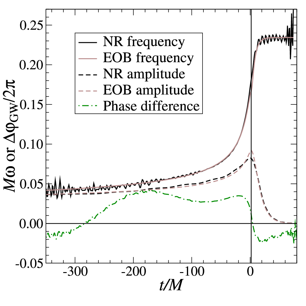

Figure 9, taken from Buonanno et al., gives an example of how well the waveforms match one another. Over the entire span computed, the two waveforms differ in phase by only a few hundredths of a cycle. The agreement is so good that one can realistically imagine “calibrating” the effective one-body waveforms with a relatively small number of expensive numerical relativity computations, and then densely sampling the binary parameter space using the effective one-body approach.
7 Gravitational-wave recoil
That GWs carry energy and angular momentum from a binary, driving its members to spiral together as described in Sec. 3.3, is widely appreciated. Until recently, it was not so well appreciated that the waves can carry linear momentum as well. If the binary and its radiation pattern are asymmetric, then that radiation carries a net flux of momentum given by
| (150) |
where is the energy-flux component of the Isaacson tensor (72), is the -th component of the radial unit vector, and the integral is taken over a large sphere () around the source. Recent work has shown that the contribution to this “kick” from the final plunge and merger of coalescing black holes can be particularly strong. We now summarize the basic physics of this effect, and survey recent results.
Bekenstein (1973) appears to have first appreciated that the momentum flux of GWs could have interesting astrophysical consequences. Fitchett (1983) then estimated the impact this flux could have on a binary. An aspect of the problem which Fitchett’s analysis makes very clear is that the recoil comes from the beating of different multipolar contributions to the recoil: If one only looks at the quadrupole part of the GWs [cf. Eq. (54)], the momentum flux is zero. Fitchett’s analysis included octupole and current-quadrupole radiation, and found
| (151) |
where gives the dependence on mass ratio . This function has a maximum at . The radius describes when wave emission cuts off; for systems containing black holes this will scale with the total mass. Thus, the recoil does not depend on total mass, just mass ratio.
Fitchett’s analysis is similar to our discussion in Sec. 3.3 in that Newtonian dynamics are supplemented with multipolar wave emission. Because the effect is strongest when is smallest, it was long clear that a proper relativistic analysis was needed to get this kick correct. Indeed, a prescient analysis by Redmount & Rees (1989) suggested that binaries containing rapidly spinning black holes were likely to be especially interesting; as we shall see in a few moments, they were absolutely correct.
Favata, Hughes & Holz (2004) provided the first estimates of recoil which did the strong-field physics more-or-less correctly. They used the perturbative techniques described in Sec. 4, arguing that one can extrapolate from the small mass ratio regime to or so with errors of a few tens of percent. Unfortunately, their code at that time did not work well with plunging orbits, so they had large error bars. They did find, however, that the maximum recoil probably fell around km/sec, at least if no more than one body spins, and if the spin and orbit are aligned. Blanchet, Qusailah & Will (2005) revisited this treatment, with a particular eye on the final plunge waves, using the pN methods outlined in Sec. 5. Their results were consistent with Favata et al., but reduced the uncertainty substantially, finding a maximum recoil km/sec.
These numbers stood as the state-of-the-art in black hole recoil for several years, until numerical relativity’s breakthrough (Sec. 6) made it possible to study black hole mergers without any approximations. The Favata et al. and Blanchet et al. numbers turn out to agree quite well with predictions for the merger of non-spinning black holes; González et al. (2007b) find the maximum kick for non-spinning merger comes when , yielding km/sec. When spin is unimportant, kicks appear to be no larger than a few hundred km/sec.
When spin is important, the kick can be substantially larger. Recent work by González et al. (2007a) and Campanelli et al. (2007) shows that when the holes have large spins and those spins are aligned just right (equal in magnitude, antiparallel to each other, and orthogonal to the orbital angular momentum), the recoil can be a few thousand km/sec. Detailed parameter exploration is needed to assess how much of this maximum is actually achieved; early work on this problem is finding that large kicks (many hundreds to a few thousand of km/sec) can be achieved for various spin orientations as long as the spins are large (Tichy & Marronetti 2007, Pollney et al. 2007); recent work by Boyle, Kesden & Nissanke (2008) shows how the recoil can depend on spin and spin orientation, suggesting a powerful way to organize the calculation to see how generic such large kicks actually are. That the maximum is so much higher than had been appreciated suggests that substantial recoils may be more common than the Favata et al. and Blanchet et al. calculations led us to expect (Schnittman & Buonanno 2007).
Many recent papers have emphasized that kicks could have strong astrophysical implications, ranging from escape of the black hole from its host galaxy to shocks in material accreting onto the large black hole. The first possible detection of black hole recoil was recently announced (Komossa, Zhou & Lu 2008). As that claim is assessed, we anticipate much activity as groups continue to try to identify a signature of a recoiling black hole.
8 Astronomy with gravitational waves
Direct GW measurement is a major motivator for theorists seeking to understand how binary systems generate these waves. The major challenge one faces is that GWs are extremely weak; as we derive in detail in this section, a wave’s strain sets the change in length per length in the arms of a GW detector. Referring to Eq. (89), we now estimate typical amplitudes for binary sources:
| (152) | |||||
On the last two lines, we have specialized to a binary whose members each have mass , and have inserted fiducial numbers corresponding to targets for ground-based detectors (second line) and space-based detectors (third line).
In the remainder of this section, we summarize the principles behind modern interferometric GW detectors. Given that these principles are likely to be novel for much of the astronomical community, we present this material in some depth. Note that Finn (2009) has recently flagged some important issues in the “standard” calculation of an interferometer’s response to GWs (which, however, do not change the final results). For the sake of brevity, we omit these issues and recommend his article for those wishing a deeper analysis. We then briefly describe existing and planned detectors, and describe how one measures a binary’s signal with these instruments. This last point highlights why theoretical modeling has been so strongly motivated by the development of these instruments.
8.1 Principles behind interferometric GW antennae
As a simple limit, treat the spacetime in which our detector lives as flat plus a simple GW propagating down our coordinate system’s -axis:
| (153) |
where . We neglect the influence of the earth (clearly important for terrestrial experiments) and the solar system (which dominates the spacetime of space-based detectors). Corrections describing these influences can easily be added to Eq. (153); we neglect them, as they represent influences that vary on much longer timescales than the GWs.

Figure 10 sketches an interferometer that can measure a GW. Begin by examining the geodesics describing the masses at the ends of the arms, and the beam splitter at the center. Take these objects to be initially at rest, so that . The GW shifts this velocity by an amount of order the wave strain: . Now examine the geodesic equation:
| (154) |
All components of the connection are . Combining this with our argument for how the GW affects the various velocities, we have
| (155) |
Now,
| (156) |
as the relevant metric components are constant. Thus,
| (157) |
The test masses are unaccelerated to leading order in the GW amplitude .
This seems to say that the GW has no impact on the masses. However, the geodesic equation describes motion with respect to a specified coordinate system. These coordinates are effectively “comoving” with the interferometer’s components. This is convenient, as the interferometer’s components remain fixed in our coordinates. Using this, we can show that the proper length of the arms does change. For instance, the -arm has a proper length
| (158) |
Likewise, the -arm has a proper length .
This result tells us that the armlengths as measured by a ruler will vary with . One might worry, though, that the ruler will vary, cancelling the measurement. This does not happen because rulers are not made of freely-falling particles: The elements of the ruler are bound to one another and act against the GW. The ruler will feel some effect from the GW, but it will be far smaller than the variation in the separation.
The ruler used by the most sensitive current and planned detectors is based on laser interferometry. We now briefly outline how a GW imprints itself on the phase of the interferometer sketched in Fig. 10. For further discussion, we recommend Faraoni (2007); we also recommend Finn (2009) for more detailed discussion. In the interferometer shown, laser light enters from the left, hits the beam splitter, travels down both the - and -arms, bounces back, and is recombined at the beam splitter. Begin with light in the -arm, and compute the phase difference between light that has completed a round trip and light that is just entering. The phase of a wavefront is constant as it follows a ray through spacetime, so we write this difference as
| (159) |
where is the laser frequency measured by an observer at the beam splitter. Detecting a GW is essentially precision timing, with the laser acting as our clock.
Consider first the proper frequency. Light energy as measured by some observer is , where is the light’s 4-momentum and is the observer’s 4-velocity. We take this observer to be at rest, so
| (160) |
Put , where describes the light in the absence of a GW, and is a GW shift. In the -arm, ; the signs correspond to before and after bounce. We compute the shift using the geodesic equation (12):
| (161) |
(We use in the background to simplify.) Focus on the component. The only nontrivial connection is . Using in addition the facts that plus reduces the geodesic equation to
| (162) |
Integrating over a round trip, we find
| (163) |
So, we finally find the proper frequency:
| (164) | |||||
On the second line of Eq. (164), we take to be much smaller than the wave period. This is an excellent approximation for ground-based interferometers; the exact result must be used for high-frequency response in space.
Turn next to the proper round-trip time. The metric (153) shows us that proper time measured at fixed coordinate is identical to the coordinate time . For light traveling in the -arm, , so
| (165) |
Now integrate over from to and back, and over from to :
| (166) | |||||
We thus find
| (167) | |||||
The second line describes a wave which barely changes during a round trip.
The total phase change is found by combining Eqs. (159), (164) and (167):
| (168) | |||||
The second line is for a slowly varying wave, and the first is exact to order . We will use the slow limit in further calculations. Repeating for the -arm yields
| (169) |
Notice that this GW acts antisymmetrically on the arms. By contrast, any laser phase noise will be symmetric: because the same laser state is sent into the arms by the beam splitter, we have . We take advantage of this by reading out light produced by destructive interference at the beamsplitter:
| (170) | |||||
An L-shaped interferometer is sensitive only to the GW, not to laser phase noise. This is the major reason that this geometry is used; even if an incident wave is oriented such that the response of the arms to the GW is not asymmetric, one is guaranteed that phase noise will be cancelled by this configuration.
From basic principles we turn now to a brief discussion of current and planned detectors. Our goal is not an in-depth discussion, so we refer readers interested in these details to excellent reviews by Hough & Rowan (2000) (which covers in detail the characteristics of the various detectors) and Tinto & Dhurandar (2005) (which covers the interferometry used for space-based detectors).
8.2 Existing and planned detectors
When thinking about GW detectors, a key characteristic is that the frequency of peak sensitivity scales inversely with armlength. The ground-based detectors currently in operation (and undergoing or about to undergo upgrades) are sensitive to waves oscillating at 10s – 1000s of Hertz. Planned space-based detectors will have sensitivities at much lower frequencies, ranging from – 0.1 Hz (corresponding to waves with periods of tens of seconds to hours).
The ground-based detectors currently in operation are LIGO (Laser Interferometer Gravitational-wave Observatory), with antennae in Hanford, Washington and Livingston, Louisiana; Virgo near Pisa, Italy; and GEO near Hanover, Germany. The LIGO interferometers each feature 4-kilometer arms, and have a peak sensitivity near 100 Hz. Virgo is similar, with 3-kilometer arms and sensitivity comparable to the LIGO detectors. GEO (or GEO600) has 600-meter arms; as such, its peak sensitivity is at higher frequencies than LIGO and Virgo. By using advanced interferometry techniques, it is able to achieve sensitivity competitive with the kilometer-scale instruments. All of these instruments will be upgraded over the course of the next few years, installing more powerful lasers, and reducing the impact of local ground vibrations. The senstivity of LIGO should be improved by roughly a factor of ten, and the bandwidth increased as well. See Fritschel (2003) for detailed discussion.
There are also plans to build additional kilometer-scale instruments. The detector AIGO (Australian International Gravitational Observatory) is planned as a detector very similar to LIGO and Virgo, but in Western Australia (McClelland 2002). This location, far from the other major GW observatories, has great potential to improve the ability of the worldwide GW detector network to determine the characteristics of GW events (Searle et al. 2006). In particular, AIGO should be able to break degeneracies in angles that determine a source’s sky position and polarization, greatly adding to the astronomical value of GW observations. The Japanese GW community, building on their experience with the 300-meter TAMA interferometer, hopes to build a 3-kilometer underground instrument. Dubbed LCGT (Large-scale Cryogenic Gravitational-wave Telescope), the underground location takes advantage of the fact that local ground motions tend to decay fairly rapidly as we move away from the earth’s surface. They plan to use cryogenic cooling to reduce noise from thermal vibrations.
In space, the major project is LISA (Laser Interferometer Space Antenna), a 5-million kilometer interferometer under development as a joint NASA-ESA mission. LISA will consist of three spacecraft placed in orbits such their relative positions form an equilateral triangle whose centroid lags the earth by , and whose plane is inclined to the ecliptic by ; see Fig. 11. Because the spacecraft are free, they do not maintain this constellation precisely; however, the variations in armlength occur on a timescale far longer than the periods of their target waves, and so can be modeled out without too much difficulty. The review by Tinto & Dhurandar (2005) discusses in great detail how one does interferometry on such a baseline with time-changing armlengths. LISA is being designed to target waves with periods of several hours to several seconds, a particularly rich band for signals involving black holes that have ; the LISA Pathfinder, a testbed for some of the mission’s components, is scheduled for launch in the very near future (Vitale 2005).

Somewhat smaller than LISA, The Japanese GW community has proposed DECIGO (DECI-hertz Gravitational-wave Observatory), a space antenna to target a band at roughly Hz. This straddles the peak sensitivities of LISA and terrestrial detectors, and may thus act as a bridge for signals that evolve from one band to the other. See Kawamura et al. (2006) for further discussion.
It’s worth nothing that, in addition to the laser interferometers discussed here, there have been proposals to measure GWs using atom interferometry. A particularly interesting proposal has been developed by Dimopoulos et al. (2008). Sources of noise in such experiments are quite different than in the case of laser interferometers, and may usefully complement the existing suite of detectors in future applications.
8.3 Measuring binary signals
The central principle guiding the measurement of GWs is that their weakness requires phase coherent signal measurement. This is similar to how one searches for a pulsar in radio or x-ray data. For pulsars, one models the signal as a sinusoid with a phenomenological model for frequency evolution:
| (171) |
The cross correlation of a model, , with data is maximized when the parameters accurately describe a signal’s phase. For a signal that is cycles long, it is not too difficult to show that the cross-correlation is enhanced by roughly when the “template” matches the data.
For binary GWs, one similarly cross-correlates models against data, looking for the template which maximizes the correlation. [Given the signal weakness implied by Eq. (152), the cross-correlation enhancement is sure to be crucial for measuring these signals in realistic noise.] Imagine, for example, that the rule given by Eq. (90) accurately described binary orbits over the band of our detectors. We would then expect a model based on
| (172) |
to give a large correlation when the coalescence phase , coalescence time , and chirp mass are chosen well. As we have discussed at length, Eq. (90) is not a good model for strong-field binaries. The need to faithfully track what nature throws at us has been a major motivation for the developments in perturbation theory, pN theory, and numerical relativity discussed here.
When one determines that some set of parameters maximizes the correlation, that set is an estimator for the parameters of the binary. More formally, the cross-correlation defines a likelihood function, which gives the probability of measuring some set of parameters from the data (Finn 1992). By examining how sharply the likelihood falls from this maximum, one can estimate how accurately data determines parameters. For large cross-correlation (large signal-to-noise ratio), this is simply related to how the wave models vary with parameters. Let represent the -th parameter describing a waveform . If denotes the cross-correlation of with itself, then define the covariance matrix
| (173) |
(where the power denotes matrix inverse). Diagonal elements of this matrix are parameter errors; off-diagonal elements describe parameter correlations. See Finn (1992) for derivations and much more detailed discussion. In the discussion that follows, we use Eq. (173) to drive the discussion of how model waveforms are used to understand how well observations will be able to determine the properties of GW-generating systems.
8.4 What we learn by measuring binary GWs
8.4.1 Overview
Given all that we have discussed, what can we learn by observing compact binary merger in GWs? To set the context, consider again the “Newtonian” waveform:
| (174) |
A given interferometer measures a combination of these two polarizations, with the weights set by the interferometers antenna response functions:
| (175) |
The angles give a sources position on the sky; the angle (in combination with ) describes the orientation of the binary’s orbital plane with respect to a detector. See Thorne (1987), Eqs. (103) – (104) for further discussion.
Imagine that Eq. (174) accurately described GWs in nature. By matching phase with the data, measurement of the GW would determine the chirp mass . Calculations using Eq. (173) to estimate measurement error (Finn & Chernoff 1993) show that should be determined with exquisite accuracy, , where is the number of GW cycles measured in our band.
The amplitude of the signal is determined with an accuracy . This means that, for a given GW antenna, a combination of the angles , , , , and the source distance are measured with this precision; however, those parameters are not invidually determined. A single interferometer cannot break the distance-angle correlations apparent in Eqs. (174) and (175). Multiple detectors (which will each have their own response functions and ) are needed to measure these source characteristics. This is one reason that multiple detectors around the globe are being built. (For LISA, the constellation’s motion around the sun makes and effectively time varying. The modulation imposed by this time variation means that the single LISA antenna can break these degeneracies, provided that a source is sufficiently long-lived for the antenna to complete a large fraction of an orbit.)
As we have discussed, Eq. (174) does not give a good description of GWs from strong-field binaries. Effects which this “Newtonian gravity plus quadrupole waves” treatment misses come into play. Consider the pN phase function, Eq. (127). Not only does the chirp mass influence the phase; so too does the binary’s reduced mass and its “spin-orbit” and “spin-spin” parameters and . The pN phasing thus encodes more detail about the binary’s characteristics. Unfortunately, these parameters may be highly correlated. For example, Cutler & Flanagan (1994) show that when precession is neglected, errors in a binary’s reduced mass and spin-orbit parameter are typically or more correlated with each other. This is because the time dependence of their contributions to the phase is not very different.
These correlations can be broken when we make our models more complete. As we’ve discussed, the spin precession equations (124) and (125) cause and to oscillate. This modulates the waves’ phase; as first demonstrated by Vecchio (2004) and then examined in greater depth by Lang & Hughes (2006), the modulations break parameter degeneracies and improve our ability to characterize the system whose waves we measure. Figure (12), taken from Lang & Hughes (2006), shows this effect for LISA measurements of coalescing binary black holes. Accounting for precession improves the accuracy with which the reduced mass is measured by roughly two orders of magnitude. We similarly find that the members’ spins can be determined with excellent accuracy. GW measurements will be able to map the mass and spin distributions of coalescing binaries.

Equation (174) is also deficient in that only the leading quadrupole harmonic is included. As the discussion in Sec. 5.2.1 demonstrates, that is just one harmonic among many that contribute to a binary’s GWs. Recent work (Arun et al. 2007, Trias & Sintes 2008, Porter & Cornish 2008) has looked at how our ability to characterize a source improves when those “higher harmonics” are included. Typically, one finds that these harmonics improve our ability to determine a binary’s orientation . This is largely because each harmonic has a slightly different functional dependence on , so each encodes that information somewhat differently than the others. The unique functional dependence of each harmonic on in turn helps break degeneracies between that angle and the source distance .
8.4.2 “Bothrodesy”: Mapping black hole spacetimes
Extreme mass ratio captures may allow a unique GW measurement: We may use them to “map” the spacetimes of large black holes and test how well they satisfy the (rather stringent) requirements of GR. As discussed in Sec. 4, an extreme mass ratio inspiral is essentially a sequence of orbits. Thanks to the mass ratio, the small body moves through this sequence slowly, spending a lot of time “close to” any orbit in the sequence. Also thanks to the mass ratio, each orbit’s properties are mostly determined by the larger body. In analogy to geodesy, the mapping of earth’s gravity with satellite orbits, one can imagine bothrodesy55 5 This name was coined by Sterl Phinney, and comes from the word , which refers to a sacrificial pit in ancient Greek. This author offers an apology to speakers of modern Greek., the mapping of a black hole’s gravity by studying the orbits of inspiraling “satellites.”
In more detail, consider first Newtonian gravity. The exterior potential of a body of radius can be expanded in a set of multipole moments:
| (176) |
Studying orbits allows us to map the potential , and thus to infer the moments . By enforcing Poisson’s equation in the interior, , and then matching at the surface , one can relate the moments to the distribution of matter. In this way, orbits allow us to map in detail the distribution of matter in a body like the earth.
Bothrodesy applies the same basic idea to a black hole. The spacetime of any stationary, axisymmetric body can be described by a set of “mass moments” , similar to the of Eq. (176); and a set of “current moments” which describe the distribution of mass-energy’s flow. What makes this test powerful is that the moments of a black hole take a simple form: for a Kerr black hole (101) with mass and spin parameter ,
| (177) |
A black hole has a mass moment and a current moment (i.e., the magnitude of its spin is , modulo factors of and ). Once those moments are known, all other moments are fixed if the Kerr solution describes the spacetime. This is a restatement of the “no hair” theorem (Carter 1971, Robinson 1975) that a black hole’s properties are set by its mass and spin.
The fact that an object’s spacetime (and hence orbits in that spacetime) is determined by its multipoles, and that the Kerr moments take such a simple form, suggests a simple consistency test: Develop an algorithm for mapping a large object’s moments by studying orbits of that object, and check that the moments satisfy Eq. (177). Ryan (1995) first demonstrated that such a measurement can in principle be done, and Brink (2008) has recently clarified what must be done for such measurements to be done in practice. Collins & Hughes (2004) took the first steps in formulating this question as a null experiment (with the Schwarzschild solution as the null hypothesis). Glampedakis & Babak (2006) formulated a similar approach appropriate to Kerr black holes, and Vigeland (Vigeland & Hughes, in preparation) has recently extended the Collins & Hughes formalism in that direction.
A robust test of the Kerr solution is thus a very likely outcome of measuring waves from extreme mass ratio captures. If, however, testing metrics is not your cup of tea, precision black hole metrology may be: In the process of mapping a spacetime, one measures with exquisite accuracy both the mass and the spin of the large black hole. Barack & Cutler (2004) have found that in most cases these events will allow us to determine both the mass and the spin of the large black hole with errors are better.
8.4.3 Binary inspiral as a standard “siren.”
A particularly exciting astronomical application of binary inspiral comes from the fact that the GWs depend on, and thus directly encode, distance to a source. Binary inspiral thus acts as a standard candle (or “standard siren,” so named because it is often useful to regard GWs as soundlike), with GR providing the standardization. Schutz (1986) first demonstrated the power of GW observations of merging binaries to pin down the Hubble constant; Marković (1993) and Finn & Chernoff (1993) analyzed Schutz’s argument in more detail, in addition assessing how well other cosmological parameters could be determined. More recently, Holz & Hughes (2005) have examined what can be done if a GW merger is accompanied by an “electromagnetic” counterpart of some kind. We now describe how inspiral waves can serve as a standard siren.
Imagine that we measure a nearby source, so that cosmological redshift can be neglected. The measured waveform generically has a form
| (178) |
where are the binary’s masses, are its spins, and is a function of the masses with dimension mass. For example, for the Newtonian quadrupole waveform (89), this function is the chirp mass, . The function is a slowly varying, dimensionless function which depends most strongly on parameters such as the source inclination .
Now place this source at a cosmological distance. Careful analysis shows that the naive Euclidean distance measure should be the proper motion distance (Carroll 2004, Chap. 8); see, e.g., Finn & Chernoff (1993) for a derivation. Also, all timescales which characterize the source will be redshifted: If is a timescale characterizing the source’s internal dynamics, .
What is the phase for this cosmological binary? Because it evolves solely due to gravity, any parameter describing the binary’s dynamics enters as a timescale. For example, a mass parameter becomes a time: . This time suffers cosmological redshift; the mass that we infer by measuring it is likewise redshifted: . Spin variables pick up a squared reshift factor: . This tells us is that redshift ends up degenerate with other parameters: A binary with masses and spins at redshift has a phase evolution that looks just like a binary with , in the local universe. So, if we put our source at redshift , Eq. (178) becomes
| (179) |
Recall that proper motion distance is related to luminosity distance by . Because we don’t measure masses but rather times masses, it makes sense to adjust the amplitude and put
| (180) |
The key point here is that measurements directly encode the luminosity distance to a source, ; however, they do not tell us anything about a source’s redshift . In this sense GW measurements of merging binaries can be distance probes that are highly complementary to most other astronomical distance measures. Indeed, analyses indicate that the distance should be measured to accuracy using ground-based instruments (e.g., Cutler & Flanagan 1994), and to from space (Lang & Hughes 2006, Arun et al. 2007, Trias & Sintes 2008, Porter & Cornish 2008).
Suppose that we measure GWs from a merging compact binary, allowing us to measure with this accuracy. If it is possible to measure the source’s redshift [either from the statistical properties of the distribution of events, as emphasized by Schutz (1986) and Chernoff & Finn (1993), or by direct association with an “electromagnetic” event (Holz & Hughes 2005)], then one may be able to accurately determine both distance and redshift for that event — a potentially powerful constraint on the universe’s cosmography with completely different systematic properties than other standard candles. An example of an event which may constitute such a standard siren is a short-hard gamma-ray burst. Evidence has accumulated recently consistent with the hypothesis that at least some short-hard bursts are associated with NS-NS or NS-BH mergers (e.g., Fox et al. 2005, Nakar, Gal-Yam & Fox 2006, Perley et al. 2008). Near simultaneous measurement of a GW signal with a short-hard burst is a perfect example of what can be done as these detectors reach maturity and inaugurate GW astronomy.
Acknowledgments
I thank Daniel Kennefick for helpful discussion about the history of this field, Thomas Baumgarte and Stuart Shapiro for teaching me most of what I know about the foundations of numerical relativity, Vicky Kalogera and Fred Rasio for helping me untangle some of the literature on rate estimates for compact binary mergers, Alessandra Buonanno for providing figures and background for the material on the effective one-body approach, Plamen Fiziev for pointing out that Chandrasekhar’s massive tome develops Kerr perturbations in the language of metric variables, and Daniel Holz and Samaya Nissanke for providing particularly thorough comments on an early draft of this paper. Some of this material was presented at the 2008 Summer School in Cosmology at the Abdus Salam International Center for Theoretical Physics, in Trieste, Italy; I thank the organizers of that school for the invitation and for the opportunity to develop and organize this material. The work I have discussed here owes a particular debt to my collaborators Neil Cornish, Steve Drasco, Marc Favata, Éanna Flanagan, Joel Franklin, Daniel Holz, Gaurav Khanna, and Samaya Nissanke; as well as to current and former graduate students Nathan Collins, Ryan Lang, Stephen O’Sullivan, Pranesh Sundararajan, and Sarah Vigeland. Finally, I thank Deepto Chakrabarty for five years of teasing, which inspired me to insert the factors of and included in the equations here. My research in gravitational waves and compact binaries is supported by NSF Grant PHY-0449884 and NASA Grant NNX08AL42G. Some of the work discussed here was also supported by NASA Grant NNG05G105G and the MIT Class of 1956 Career Development Fund.
References
- Armitage & Natarajan (2002) Armitage PJ, Natarajan P. 2002. Astrophys. J. Lett. 567:L9–L12
- Arnowitt, Deser & Misner (1962) Arnowitt R, Deser S, Misner CW. 1962. In Gravitation: An introduction to current research, ed. L Witten
- Arun et al. (2007) Arun KG, Iyer BR, Sathyaprakash BS, Sinha S, van den Broeck C. 2007. Phys. Rev. D 76:104016
- Baiotti, Giacomazzo & Rezzolla (2008) Baiotti L, Giacomazzo B, Rezzolla L. 2008. Phys. Rev. D 78:084033
- Baker et al. (2007) Baker JG, Campanelli M, Pretorius F, Zlochower Y. 2007. Class. Quantum Grav. 24:25
- Baker et al. (2006) Baker JG, Centrella J, Choi DI, Koppitz M, van Meter J. 2006. Phys. Rev. Lett. 96:111102
- Barack & Cutler (2004) Barack L, Cutler C. 2004. Phys. Rev. D 69:082005
- Barack & Sago (2007) Barack L, Sago N. 2007. Phys. Rev. D 75:064021
- Baumgarte & Shapiro (1999) Baumgarte TW, Shapiro SL. 1999. Phys. Rev. D 59:024007
- Baumgarte & Shapiro (2003) Baumgarte TW, Shapiro SL. 2003. Phys. Rep. 376:41
- Begelman, Blandford & Rees (1980) Begelman MC, Blandford RD, Rees MJ. 1980. Nature 287:307–309
- Bekenstein (1973) Bekenstein JD. 1973. Astrophys. J. 183:657
- Bhat, Bailes & Verbiest (2008) Bhat NDR, Bailes M, Verbiest JPW. 2008. Phys. Rev. D 77:124017
- Blanchet (2006) Blanchet L. 2006. Living Reviews in Relativity 9:4
- Blanchet et al. (1995) Blanchet L, Damour T, Iyer BR, Will CM, Wiseman AG. 1995. Phys. Rev. Lett. 74:3515–3518
- Blanchet, Qusailah & Will (2005) Blanchet L, Qusailah MSS, Will CM. 2005. Astrophys. J. 635:508–515
- Boyle, Kesden & Nissanke (2008) Boyle L, Kesden M, Nissanke S. 2008. Phys. Rev. Lett. 100:151101
- Brink (2008) Brink J. 2008. Phys. Rev. D 78:102001
- Brügmann, Tichy & Jansen (2004) Brügmann B, Tichy W, Jansen N. 2004. Phys. Rev. Lett. 92:211101
- Buonanno & Damour (1999) Buonanno A, Damour T. 1999. Phys. Rev. D 59:084006
- Buonanno et al. (2007) Buonanno A, Pan Y, Baker JG, Centrella J, Kelly BJ, et al. 2007. Phys. Rev. D 76:104049
- Campanelli et al. (2006) Campanelli M, Lousto CO, Marronetti P, Zlochower Y. 2006. Phys. Rev. Lett. 96:111101
- Campanelli et al. (2007) Campanelli M, Lousto CO, Zlochower Y, Merritt D. 2007. Phys. Rev. Lett. 98:231102
- Carroll (2004) Carroll S. 2004. Spacetime and Geometry: An introduction to general relativity. San Francisco: Addison-Wesley, 1st ed.
- Carter (1971) Carter B. 1971. Phys. Rev. Lett. 26:331
- Chandrasekhar (1983) Chandrasekhar S. 1983. The mathematical theory of black holes. New York: Oxford University Press
- Chernoff & Finn (1993) Chernoff DF, Finn LS. 1993. Astrophys. J. Lett. 411:L5
- Collins & Hughes (2004) Collins NA, Hughes SA. 2004. Phys. Rev. D 69:124022
- Conway & Wrobel (1995) Conway JE, Wrobel JM. 1995. Astrophys. J. 439:98
- Cutler & Flanagan (1994) Cutler C, Flanagan ÉE. 1994. Phys. Rev. D 49:2658
- Damour (1983a) Damour T. 1983a. In Gravitational radiation; Proceedings of the Advanced Study Institute, Les Houches, Haute-Savoie, France, June 2-21, 1982, eds. N Deruelle, T Piran
- Damour (1983b) Damour T. 1983b. Physical Review Letters 51:1019–1021
- Damour (2008) Damour T. 2008. International Journal of Modern Physics A 23:1130–1148
- Damour, Iyer & Sathyaprakash (1998) Damour T, Iyer BR, Sathyaprakash BS. 1998. Phys. Rev. D 57:885
- Damour et al. (2008) Damour T, Nagar A, Hannam M, Husa S, Brügmann B. 2008. Phys. Rev. D 78:044039
- Detweiler (2008) Detweiler S. 2008. Phys. Rev. D 77:124026
- Dewitt & Brehme (1960) Dewitt BS, Brehme RW. 1960. Annals of Physics 9:220–259
- Di Matteo et al. (2008) Di Matteo T, Colberg J, Springel V, Hernquist L, Sijacki D. 2008. Astrophys. J. 676:33–53
- Dimopoulos et al. (2008) Dimopoulos S, Graham PW, Hogan JM, Kasevich MA, Rajendran S. 2008. Phys. Rev. D 78:122002
- Dirac (1938) Dirac PAM. 1938. Proc. Roy. Soc. Lond. A167:148–169
- Drasco & Hughes (2004) Drasco S, Hughes SA. 2004. Phys. Rev. D 69:044015
- Drasco & Hughes (2006) Drasco S, Hughes SA. 2006. Phys. Rev. D 73:024027
- Eddington (1922) Eddington AS. 1922. Proc. Roy. Soc. Lond. A102:268–282
- Ehlers et al. (1976) Ehlers J, Rosenblum A, Goldberg JN, Havas P. 1976. Astrophys. J. Lett. 208:L77
- Eichler et al. (1989) Eichler D, Livio M, Piran T, Schramm DN. 1989. Nature 340:126
- Etienne et al. (2008) Etienne ZB, Faber JA, Liu YT, Shapiro SL, Taniguchi K, Baumgarte TW. 2008. Phys. Rev. D 77:084002
- Faraoni (2007) Faraoni V. 2007. Gen. Rel. Grav. 39:677
- Favata, Hughes & Holz (2004) Favata M, Hughes SA, Holz DE. 2004. Astrophys. J. Lett. 607:L5
- Ferrarese (2002) Ferrarese L. 2002. In Current high-energy emission around black holes, eds. CH Lee, HY Chang
- Finn (1992) Finn LS. 1992. Phys. Rev. D 46:5236
- Finn (2009) Finn LS. 2009. Phys. Rev. D 79:022002
- Finn & Chernoff (1993) Finn LS, Chernoff DF. 1993. Phys. Rev. D 47:2198
- Fitchett (1983) Fitchett MJ. 1983. Mon. Not. R. Astron. Soc. 203:1049–1062
- Fiziev (2009) Fiziev PP. 2009. ArXiv e-prints
- Flanagan & Hughes (1998) Flanagan ÉÉ, Hughes SA. 1998. Phys. Rev. D 57:4535
- Flanagan & Hughes (2005) Flanagan ÉÉ, Hughes SA. 2005. New Journal of Physics 7:204
- Fox et al. (2005) Fox DB, Frail DA, Price PA, Kulkarni SR, Berger E, et al. 2005. Nature 437:845
- Fritschel (2003) Fritschel P. 2003. In Society of Photo-Optical Instrumentation Engineers (SPIE) Conference Series, eds. M Cruise, P Saulson, vol. 4856 of Society of Photo-Optical Instrumentation Engineers (SPIE) Conference Series
- Ganz et al. (2007) Ganz K, Hikida W, Nakano H, Sago N, Tanaka T. 2007. Prog. Theor. Phys. 117:1041
- Gerke et al. (2007) Gerke BF, Newman JA, Lotz J, Yan R, Barmby P, et al. 2007. Astrophys. J. Lett. 660:L23
- Glampedakis & Babak (2006) Glampedakis K, Babak S. 2006. Class. Quantum Grav. 23:4167
- González et al. (2007a) González JA, Hannam M, Sperhake U, Brügmann B, Husa S. 2007a. Phys. Rev. Lett. 98:231101
- González et al. (2007b) González JA, Sperhake U, Brügmann B, Hannam M, Husa S. 2007b. Phys. Rev. Lett. 98:091101
- Haiman, Ciotti & Ostriker (2004) Haiman Z, Ciotti L, Ostriker JP. 2004. Astrophys. J. 606:763–773
- Holz & Hughes (2005) Holz DE, Hughes SA. 2005. Astrophys. J. 629:15
- Hopkins et al. (2008) Hopkins PF, Cox TJ, Kereš D, Hernquist L. 2008. Astrophys. J. Suppl. 175:390–422
- Hopman & Alexander (2005) Hopman C, Alexander T. 2005. Astrophys. J. 629:362–372
- Hough & Rowan (2000) Hough J, Rowan S. 2000. Liv. Rev. Rel. 3:3
- Hughes (2000) Hughes SA. 2000. Phys. Rev. D 61:084004
- Hughes et al. (2005) Hughes SA, Drasco S, Flanagan EE, Franklin J. 2005. Phys. Rev. Lett. 94:221101
- Hulse & Taylor (1975) Hulse RA, Taylor JH. 1975. Astrophys. J. Lett. 195:L51
- Isaacson (1968) Isaacson RA. 1968. Physical Review 166:1272
- Jackson (1975) Jackson JD. 1975. Classical electrodynamics. 92/12/31, New York: Wiley, 1975, 2nd ed.
- Jacoby et al. (2006) Jacoby BA, Cameron PB, Jenet FA, Anderson SB, Murty RN, Kulkarni SR. 2006. Astrophys. J. Lett. 644:L113–L116
- Kalogera et al. (2007) Kalogera V, Belczynski K, Kim C, O’Shaughnessy R, Willems B. 2007. Physics Reports 442:75
- Kasian (2008) Kasian L. 2008. In 40 Years of Pulsars: Millisecond Pulsars, Magnetars and More, eds. C Bassa, Z Wang, A Cumming, VM Kaspi, vol. 983 of American Institute of Physics Conference Series
- Kawamura et al. (2006) Kawamura S, Nakamura T, Ando M, Seto N, Tsubono K, et al. 2006. Class. Quantum Grav. 23:125
- Kennefick (2007) Kennefick D. 2007. Traveling at the Speed of Thought. Princeton, New Jersey: Princeton University Press, 1st ed.
- Kim, Kalogera & Lorimer (in press) Kim C, Kalogera V, Lorimer DR. in press. In A Life with Stars — In honor of Ed van den Heuvel
- Komossa et al. (2003) Komossa S, Burwitz V, Hasinger G, Predehl P, Kaastra JS, Ikebe Y. 2003. Astrophys. J. Lett. 582:L15
- Komossa, Zhou & Lu (2008) Komossa S, Zhou H, Lu H. 2008. Astrophys. J. Lett. 678:L81
- Kormendy & Gebhardt (2001) Kormendy J, Gebhardt K. 2001. In 20th Texas Symposium on relativistic astrophysics, eds. JC Wheeler, H Martel, vol. 586 of American Institute of Physics Conference Series
- Kramer & Stairs (2008) Kramer M, Stairs IH. 2008. Ann. Rev. Astron. Astrop. 46:541–572
- Landau & Lifshitz (1975) Landau LD, Lifshitz EM. 1975. The classical theory of fields. Course of theoretical physics - Pergamon International Library of Science, Technology, Engineering and Social Studies, Oxford: Pergamon Press, 1975, 4th rev.engl.ed.
- Lang & Hughes (2006) Lang RN, Hughes SA. 2006. Phys. Rev. D 74:122001
- Leaver (1985) Leaver EW. 1985. R. Soc. Lond. Proc. Ser. A 402:285
- Lindblom & Scheel (2002) Lindblom L, Scheel MA. 2002. Phys. Rev. D 66:084014
- Liu, Wu & Cao (2003) Liu FK, Wu XB, Cao SL. 2003. Mon. Not. R. Astron. Soc. 340:411
- Lobanov & Roland (2005) Lobanov AP, Roland J. 2005. Astron. Astrophys. 431:831
- Mackey et al. (2008) Mackey AD, Wilkinson MI, Davies MB, Gilmore GF. 2008. Mon. Not. R. Astron. Soc. 386:65–95
- Maness et al. (2004) Maness HL, Taylor GB, Zavala RT, Peck AB, Pollack LK. 2004. Astrophys. J. 602:123
- Mano, Suzuki & Takasugi (1996) Mano S, Suzuki H, Takasugi E. 1996. Prog. Theo. Phys. 95:1079–1096
- Marković (1993) Marković D. 1993. Phys. Rev. D 48:4738–4756
- McClelland (2002) McClelland DE. 2002. In 9th Marcel Grossmann Meeting, eds. VG Gurzadyan, RT Jantzen, R Ruffini
- Menou, Haiman & Kocsis (2008) Menou K, Haiman Z, Kocsis B. 2008. New Astronomy Review 51:884–890
- Menou, Haiman & Narayanan (2001) Menou K, Haiman Z, Narayanan VK. 2001. Astrophys. J. 558:535–542
- Merritt & Ekers (2002) Merritt D, Ekers RD. 2002. Science 297:1310–1313
- Merritt & Milosavljević (2005) Merritt D, Milosavljević M. 2005. Living Reviews in Relativity 8:8
- Mino et al. (1997) Mino Y, Sasaki M, Shibata M, Tagoshi H, Tanaka T. 1997. Progress of Theoretical Physics Supplement 128:1
- Misner, Thorne & Wheeler (1973) Misner CW, Thorne KS, Wheeler JA. 1973. Gravitation. San Francisco: W. H. Freeman and Co., 1973
- Nagar, Damour & Tartaglia (2007) Nagar A, Damour T, Tartaglia A. 2007. Class. Quantum Grav. 24:109
- Nakar, Gal-Yam & Fox (2006) Nakar E, Gal-Yam A, Fox DB. 2006. Astrophys. J. 650:281
- Narayan, Piran & Shemi (1991) Narayan R, Piran T, Shemi A. 1991. Astrophys. J. Lett. 379:L17
- Nice et al. (2005) Nice DJ, Splaver EM, Stairs IH, Löhmer O, Jessner A, et al. 2005. Astrophys. J. 634:1242–1249
- Nissanke (2006) Nissanke S. 2006. Phys. Rev. D 73:124002
- O’Leary, O’Shaughnessy & Rasio (2007) O’Leary RM, O’Shaughnessy R, Rasio FA. 2007. Phys. Rev. D 76:061504
- Penrose (1960) Penrose R. 1960. Annals Phys. 10:171
- Perley et al. (2008) Perley DA, Metzger BD, Granot J, Butler NR, Sakamoto T, et al. 2008. ArXiv e-prints
- Peters (1964) Peters PC. 1964. Phys. Rev. 136:1224
- Peters & Mathews (1963) Peters PC, Mathews J. 1963. Physical Review 131:435–440
- Phinney (1991) Phinney ES. 1991. Astrophys. J. Lett. 380:L17
- Pollney et al. (2007) Pollney D, Reisswig C, Rezzolla L, Szilágyi B, Ansorg M, et al. 2007. Phys. Rev. D 76:124002
- Portegies Zwart & McMillan (2000) Portegies Zwart SF, McMillan SLW. 2000. Astrophys. J. Lett. 528:L17
- Porter & Cornish (2008) Porter EK, Cornish NJ. 2008. Phys. Rev. D 78:064005
- Postnov & Prokhorov (1999) Postnov KA, Prokhorov ME. 1999. ArXiv e-prints, astro-ph/9903193
- Pound, Poisson & Nickel (2005) Pound A, Poisson E, Nickel BG. 2005. Phys. Rev. D 72:124001
- Pretorius (2005) Pretorius F. 2005. Phys. Rev. Lett. 95:121101
- Pretorius (2009) Pretorius F. 2009. In Physics of relativistic objects in compact binaries: From birth to coalescence, eds. M Colpi, P Casella, V Gorini, U Moschella, vol. 359. Berlin: Springer
- Price (1972a) Price RH. 1972a. Phys. Rev. D 5:2419–2438
- Price (1972b) Price RH. 1972b. Phys. Rev. D 5:2439–2454
- Quinn & Wald (1999) Quinn TC, Wald RM. 1999. Phys. Rev. D 60:064009
- Rathore, Blandford & Broderick (2005) Rathore Y, Blandford RD, Broderick AE. 2005. Mon. Not. R. Astron. Soc. 357:834–846
- Redmount & Rees (1989) Redmount IH, Rees MJ. 1989. Comments on Astrophysics 14:165–175
- Regge & Wheeler (1957) Regge T, Wheeler JA. 1957. Phys. Rev. 108:1063
- Rezzolla (2003) Rezzolla L. 2003. ICTP Lecture Series, Vol. 3, ISBN 92-95003-05-5; gr-qc/0302025
- Robinson (1975) Robinson DC. 1975. Phys. Rev. Lett. 34:905
- Rodriguez et al. (2006) Rodriguez C, Taylor GB, Zavala RT, Peck AB, Pollack LK, Romani RW. 2006. Astrophys. J. 646:49
- Rosswog, Ramirez-Ruiz & Hix (2008) Rosswog S, Ramirez-Ruiz E, Hix R. 2008. ArXiv e-prints, arXiv:0808.2143
- Ryan (1995) Ryan FD. 1995. Phys. Rev. D 52:5707
- Ryan (1974) Ryan MP. 1974. Phys. Rev. D 10:1736
- Sago, Barack & Detweiler (2008) Sago N, Barack L, Detweiler S. 2008. Phys. Rev. D 78:124024
- Schmidt (2002) Schmidt W. 2002. Class. Quantum Grav. 19:2743
- Schnittman & Buonanno (2007) Schnittman JD, Buonanno A. 2007. Astrophys. J. Lett. 662:L63–L66
- Schutz (1986) Schutz BF. 1986. Nature 323:310
- Searle et al. (2006) Searle AC, Scott SM, McClelland DE, Finn LS. 2006. Phys. Rev. D 73:124014
- Shapiro & Teukolsky (1983) Shapiro SL, Teukolsky SA. 1983. Black holes, white dwarfs, and neutron stars: The physics of compact objects. Wiley-Interscience
- Shibata et al. (2009) Shibata M, Kyutoku K, Yamamoto T, Taniguchi K. 2009. Phys. Rev. D 79:044030
- Shibata & Nakamura (1995) Shibata M, Nakamura T. 1995. Phys. Rev. D 52:5428
- Shibata & Uryū (2006) Shibata M, Uryū K. 2006. Phys. Rev. D 74:121503
- Sigurdsson & Rees (1997) Sigurdsson S, Rees MJ. 1997. Mon. Not. R. Astron. Soc. 284:318–326
- Spitzer (1969) Spitzer LJ. 1969. Astrophys. J. Lett. 158:139
- Stairs et al. (1998) Stairs IH, Arzoumanian Z, Camilo F, Lyne AG, Nice DJ, et al. 1998. Astrophys. J. 505:352–357
- Sundararajan (2008) Sundararajan PA. 2008. Phys. Rev. D 77:124050
- Sundararajan et al. (2008) Sundararajan PA, Khanna G, Hughes SA, Drasco S. 2008. Phys. Rev. D 78:024022
- Tauris & van den Heuvel (2006) Tauris TM, van den Heuvel E. 2006. In Compact Stellar X-ray Sources, eds. W Lewin, M van der Klis. Cambridge: Cambridge University Press
- Teukolsky (1973) Teukolsky SA. 1973. Astrophys. J. 185:635
- Thorne (1980) Thorne KS. 1980. Rev. Mod. Phys. 52:299
- Thorne (1987) Thorne KS. 1987. In 300 Years of Gravitation, eds. SW Hawking, W Israel. Cambridge: Cambridge University Press
- Thorne & Hartle (1985) Thorne KS, Hartle JB. 1985. Phys. Rev. D 31:1815–1837
- Tichy & Marronetti (2007) Tichy W, Marronetti P. 2007. Phys. Rev. D 76:061502
- Tinto & Dhurandar (2005) Tinto M, Dhurandar SV. 2005. Liv. Rev. Rel. 8:4
- Trias & Sintes (2008) Trias M, Sintes AM. 2008. Phys. Rev. D 77:024030
- Valtonen et al. (2008) Valtonen MJ, Lehto HJ, Nilsson K, Heidt J, Takalo LO, et al. 2008. Nature 452:851
- Vecchio (2004) Vecchio A. 2004. Phys. Rev. D 70:042001
- Vitale (2005) Vitale S. 2005. ArXiv General Relativity and Quantum Cosmology e-prints, gr-qc/0504062
- Volonteri, Haardt & Madau (2003) Volonteri M, Haardt F, Madau P. 2003. Astrophys. J. 582:559–573
- Weinberg (1972) Weinberg S. 1972. Gravitation and Cosmology: Principles and Applications of the General Theory of Relativity. New York: Wiley
- Weisberg & Taylor (2005) Weisberg JM, Taylor JH. 2005. In Binary Radio Pulsars, eds. FA Rasio, IH Stairs, vol. 328 of Astronomical Society of the Pacific Conference Series
- Yu & Tremaine (2002) Yu Q, Tremaine S. 2002. Mon. Not. R. Astron. Soc. 335:965–976
- Yunes et al. (2006) Yunes N, Tichy W, Owen BJ, Brügmann B. 2006. Phys. Rev. D 74:104011
- Yungelson & Portegies Zwart (1997) Yungelson L, Portegies Zwart SF. 1997. In Second Workshop on Gravitational Wave Data Analysis, eds. M Davier, P Hello. Editiones Frontières
- Zerilli (1970) Zerilli FJ. 1970. Phys. Rev. D 2:2141
- Zhou et al. (2004) Zhou H, Wang T, Zhang X, Dong X, Li C. 2004. Astrophys. J. Lett. 604:L33