Instability of the Rayleigh-Jeans spectrum
in weak wave turbulence theory

Since early work that has addressed the kinetics of Bose-Einstein condensation even before the experimental realization of BEC in weakly interacting atomic gases [1, 2, 3, 4, 5], the description of the growth of the condensate has been the subject of considerable attention [6, 7, 8, 9, 10]. At the first stage of evolution, a description based on the Boltzmann kinetic equation is adequate. In the homogeneous case, it has the form

where we are using $\int_{\bm{p}}$ to denote momentum integration,

Here $n(\bm{p},t)$ is the distribution function, the average density of particles with momentum $\bm{p}$ at time $t$. The square-amplitude is taken as $|\mathcal{M}|^{2}=(8\pi am^{-1})^{2}$, with $a$ the scattering length parameterizing the Fermi pseudopotential $V(\bm{r}_{1}-\bm{r}_{2})=4\pi am^{-1}\delta(\bm{r}_{1}-\bm{r}_{2})$ appropriate to low-energy scattering by a interaction of finite range $R\gg a$. The dispersion law is $\omega(p)=\frac{p^{2}}{2m}$.

Based on the assumption that the formation of a condensate is a low energy process where the occupation numbers obey the condition $n(t,\bm{p})\gg 1$, it is customary to approximate the Boltzmann equation by the kinetic equation of wave turbulence [11, 12]

Using considerations of homogeneity [13], it is possible to obtain stationary power-law solutions $n=Bp^{-\nu}$, for the pair of values $\nu=3,7/3$. These Kolmogorov spectra are conjugate to the obvious solutions for $\nu=2,0$. However, the results of several studies [4, 8, 5, 9, 15] which have addressed the question of the dynamics underlying Eq. (3) seem to exclude any significant role of the Kolmogorov spectra in the formation of a finite time singularity corresponding to a condensate. Within the framework of kinetic theory, the dynamics before blow-up is rather described by a self-similar solution of the form $n(t,p)=\beta^{-1/2}\Phi((t_{\ast}-t)^{-\beta}/p^{2})$, where $t_{\ast}$ is the time of blow-up and the parameters $\alpha$ and $\beta$ are related by $\beta=\alpha-1/2$ (for a review, see Ref. [14]). The determination of the ratio $\alpha/\beta$ poses a very difficult nonlinear eigenvalue problem which can not be solved by scaling arguments. The numerical observed value $\alpha/\beta\approx 1.234$ is significant different from the exponents $\nu/2=3/2,7/6,1$ associated with Kolmogorov and equilibrium solutions. However, the classical Rayleigh-Jeans spectrum with zero chemical potential plays a special role as boundary in the appropriate parameter space between the regions of condensate and normal phases (see Fig. 1). To understand its significance it can be of some interest to study in detail the stability properties of this equilibrium solution.

In this paper, we address the question of the linear stability of the Rayleigh-Jeans spectrum ($\nu=2$) of (3) whose perturbations could be related to processes driving particle transport towards the region of $\bm{p}=0$. Let us remark that if one tries to use the equilibrium $n=T/\omega(p)$ in the entire interval of time, one faces a serious difficulty. Consider a prescribed total particle density $n$ to be accommodated by a singular distribution $n_{0}(T)(2\pi)^{3}\delta(\bm{p})$ and an equilibrium Rayleigh-Jeans distribution through

For a given cut-off $\Lambda$, the second term grows with $T$, and when it reaches the prescribed total density $n$, the density of particles in the $\bm{p}=0$ state vanishes. The temperature above which $n_{0}=0$ is $T_{c}=\pi^{2}n/(m\Lambda)$. In this model, the particle density in the condensate is given by

From this fact, one would expect that the Rayleigh-Jeans spectrum can not be stable with respect to changes of temperature: a small change in $T$ in the neighborhood of $T_{c}$ may move the system toward a state where $n_{0}\neq 0$ or not. Remarkably, this will be reflected by the fact that the linearized kinetic equation about $n^{0}=T/\omega(p)$ does not admit as a solution the function $A(\bm{p},t)\equiv\delta T(\bm{p},t)/T=\text{constant}$. This argument pointing out an instability does not apply to the equilibrium distribution function, $n\propto p^{-1}$, which arises as the solution of the three-wave kinetic equation at the end of the condensation process [16, 17]. This comes from to the low frequency limit of the Bogoliubov dispersion law $\omega_{B}(p)=\sqrt{4\pi ap^{2}/m+(p^{2}/(2m))^{2}}$. In that case, the distribution function $n$ corresponds to Goldstone-type excitations whose number is not conserved. Our focus will be on the regime in which the four-wave interactions are the most important. The transition from this stage to the three-wave regime has been recently studied within the two-dimensional Gross-Pitaevskii model in [18, 19]. These authors have shown that this transition involves an intermediate step where strong interactions between topological defects take place in a similar way to the Kibble-Zurek mechanism in continuous phase transitions.

It is important to point out that the evolution of an initial distribution function $n(\bm{p},t=0)$ in the regime of large occupation numbers produces a change in the entropy density

given by

which only vanishes for distribution functions with the shape of Rayleigh-Jeans. This result and the conservation laws imply that the final state of the evolution is consistent with the presence of a regular Rayleigh-Jeans distribution with or without a singular distribution, depending on whether the particle and energy densities in the initial distribution are below or above their critical values (see Fig. 1). It follows that a perturbed Rayleigh-Jeans distribution $T/\omega(p)+\delta n(\bm{p},t=0)$ can not evolve to the same $n^{0}=T/\omega(p)$ unless the energy $\delta(E/V)$ and the particle number $\delta(N/V)$ of $\delta n(\bm{p},t=0)$ vanish.

Although the theory of wave turbulence has been used in a variety of systems, ranging from ocean or capillary waves to plasma waves or elastic waves (see, for example, [20] for a short review), specific studies on the stability of the stationary spectra are rather scarce. In this respect, another objective of this work is to present a specific new application where the techniques of Ref. [12] are used.

This paper is organized as follows. In Sec. II we derive the linearized kinetic equation about the Rayleigh-Jeans spectrum. In Sec. III, we introduce the Mellin function, and present some of its properties. The character of the evolution of the perturbation is considered as $p\rightarrow 0,\infty$ and as $t\rightarrow\infty$. We also compute the leading asymptotics as $t\rightarrow\infty$ of the perturbed particle number which is contained in the interval $0\leq p\leq\Lambda$. Section IV gives our conclusions. Details of some calculations regarding the reduction of the integral equation to the Fredholm form and the evaluation of the Mellin function can be found in a pair of appendices.

Here we derive the linearized kinetic equation about the Rayleigh-Jeans spectrum

where it is understood that the temperature is at the critical value $T=T_{c}=\pi^{2}n/(m\Lambda)$ in this model. We shall closely follow the conventions of [12]. The dimensionless quantity $A(\bm{p},t)$ represents the relative change in the particle number and may be either positive or negative. Substituting the expression

into (3) and retaining the terms of $O(A)$ gives an integral equation for $A(\bm{p},t)$,

with the result

where we have used the conservation of energy

and the symmetry of the integrand under $\bm{p}_{3}\leftrightarrow\bm{p}_{4}$ to duplicate the last term. As we shall see, one must be cautious using this rearrangement, which assumes regularity of the integrand. Here we require that the solution $A(\bm{p},t)$ falls off sufficiently rapid as $p\rightarrow\infty$ to permit this kind of reordering in the integration. In the present case the several integral terms of the operator $L$ containing the function $A(\bm{p},t)$ for different arguments $\bm{p}$ are well defined separately, and it is possible to write

where the coefficient $N$ turns out to be a constant.

Due to the conservation laws, one expects that the collision integral $L[A]$ vanishes for certain forms of $A$. One of them, which reflects conservation of particle number, is $A(p)\propto p^{-2}$. This collision invariant corresponds to the fact that the kinetic equation (3) admits the Rayleigh-Jeans spectrum with non-zero chemical potential as an exact solution

which implies that $A=\mu/\omega(p)$ is a zero mode of the linearized equation and

would be true. In fact, this turns out to be the case, as we have explicitly checked in Eq.(74) of the appendix. Since the linear momentum is conserved, a possible solution of Eq. (3) is

which would imply that $A\propto\bm{v}\cdot\bm{p}$ is also a zero mode of the operator $L$.

Finally, from the conservation of the kinetic energy in collisions one would expect a zero mode $A=\textrm{constant}$ but, surprisingly, this does not occur, at least for the operator $L$ in the form (11). Consider $L[1]$ as follows from Eq. (11):

It it were allowable to make the exchange $\bm{p}_{3}\leftrightarrow\bm{p}_{4}$ in the second term, we would obtain the expected result $L[1]=0$. However, one finds that

and

These asymptotics give rise to leading divergences of the form $\ln^{2}(\Lambda/p_{1})$ for the remanining integration over $\bm{p}_{3}$ and $\bm{p}_{2}$ respectively, being $\Lambda$ an ultraviolet cutoff. This points out that it is not legitimate to use the previous rearrangement. We can see, however, that there is a cancellation between both divergences with the result that $L[1]>0$. Using the notation in Appendix A we obtain

It is convenient to expand the kernel $U(\bm{p},\bm{p}^{\prime})$ in terms of Legendre polynomials of the angle $\theta_{\bm{p}\bm{p}^{\prime}}=\hat{\bm{p}}\cdot\hat{\bm{p}^{\prime}}$,

and to expand [12] the perturbation $A$ in spherical harmonics relative to the orientation of $\bm{p}$,

From the addition theorem for spherical harmonics

and the orthogonality relation ($d\Omega_{\bm{p}^{\prime}}$ denotes the corresponding surface element of the three-dimensional unit sphere)

a set of uncoupled equations emerges, each one of them labeled by $(l,m)$:

In the homogeneous case, the angular momentum projection $m$ may be suppresed because of isotropy, and it is enough to use $l$ to label each irreducible perturbation.

Since we are only interested in the $l=0$ mode, we drop this label to simplify the notation. In order to obtain the explicit form of the integral equation we must first evaluate the integrals involved in Eq. (11). Some details of these calculations are given in Appendix A. One finds

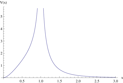
where the dimensionless constant $\gamma_{N}$ and $\tau$ with dimension of time are given in (58) and (71), respectively. The kernel $\mathcal{V}(x)$ is given in Eqs. (70), (61), (67) and is depicted in Fig. 2. This equation is a special case of the general equation which arises in the linearization of the kinetic equation about the Kolmogorov spectrum. The resulting equation has the homogeneous form [12]

In the present case, $h=0$ and $\mathcal{U}(x)$ is expressed as $\gamma_{N}\delta(x-1)+\mathcal{V}(x)$.

The Mellin transform is a very useful tool for solving the integral equation (26). In terms of the Mellin transform of $\mathcal{V}$, we define

and thus the Mellin image $\mathcal{F}(s,t)$ of $\mathcal{A}(p,t)$ is a solution to

Hereafter we will use $t$ and $p$ to denote the dimensionless variables $t/\tau$ and $p\mathit{l}$, where $\mathit{l}^{-1}$ is some momentum scale entering into the initial condition $\mathcal{A}(p,t=0)$. With these notation, the solution of the integral equation may be written as

where $\Phi(s)$ is the Mellin transform of the initial condition $\mathcal{A}(p,t=0)$

and $\sigma$ stands somewhere in $-2<\sigma<5$, corresponding to the fundamental strip where $W(s)$ is analytic. This property follows from the behavior of $\mathcal{V}(x)$

which shows that the Mellin function has double poles at $s=-2$ and $s=5$,

Some indications about the computation of the Mellin function are given in appendix B. One finds that $W(s)$ has zeros at $s=1$ and $s=2$ (see Fig. 3), with the corresponding solutions $\mathcal{A}=p^{-1},p^{-2}$. Another property is the symmetry with respect to the line $\text{Re}\,s=3/2$,

The Taylor series about $s=3/2$ reads

In this paper we have considered the problem of the stability of the Rayleigh-Jeans equilibrium solution of the theory of weak wave turbulence, in the case of the four-wave contact interactions with a non-relativistic dispersion law. It is believed that this theory captures the basics facts of the non-equililibrium processes which occur in weakly interacting Bose gases in the ‘classical’ regime where the occupation number is large.

Based on the general theory of the stability of weak-turbulence Kolmogorov spectra presented in Ref. [12], we have first derived the explicit expression for the linear evolution equation for the scalar ($l=0$) perturbations, and then we have applied the method of Mellin function to analyze the stability of solutions. Had the index $h$ been positive, the sufficient condition of Balk and Zakharov, $W(0)>0$, would immediately imply the instability of the initial perturbation in the sense of Ref. [12]. However, this effective criterion for checking the stability is inapplicable in the present case. In order to see the the character of the evolution of an arbitrary initial perturbation, we have evaluated the leading asymptotic behavior as $|\ln p\,|\rightarrow\infty$ with $t$ held fixed, and as $t\rightarrow\infty$ with $p$ held fixed. But a better understanding about the time evolution of a generic solution comes from the asymptotics for the integrated particle number as $t\rightarrow\infty$. This evaluation shows clearly the main feature of the evolution of the perturbation: the initial departure of the particle density concentrates as $t\rightarrow\infty$ into an interval of arbitrarily small width around the origin in momentum space. Let us remark again that numerical work based on the nonlinear kinetic equation (3) strongly indicates a finite time for the formation of a singularity, according to the scenario described in Refs. [5, 9, 14, 15] where the nonlinear effects are important. We must then be very cautious in seeing the asymptotic instability of the linearized equation around a Rayleigh-Jeans spectrum as a hint of the Bose-Einstein condensation.

Finally, it is worthy mentioning that natural extensions of this work include the analysis of the stability of the Rayleigh-Jeans spectrum of three-wave kinetic equations such as those that arise at the final stage of the condensation process, and the stability for $T>T_{c}$ where the chemical potential is finite. Work in this direction is in progress.

The work of M. E. is supported by the Spanish MICINN under Grant MTM2008-03541 and by the Basque Government under Grant No. IT-305-07. The work of M. A. V. is partially supported by the Spanish Consolider-Ingenio 2010 Programme CPAN (CSD2007-00042) and by the Basque Government under Grant No. IT-357-07.

References

• [1] E. Levich and V. Yakhot, Phys. Rev. B 15, 243 (1977); J. Phys. A 11, 2237 (1978).
• [2] D. W. Snoke and J. P. Wolfe, Phys. Rev. B 39, 4030 (1989).
• [3] H. T. C. Stoof, Phys. Rev. Lett. 66, 3148 (1991).
• [4] Yu. Kagan, in Bose-Einstein Condensation edited by A. Griffin, D. W. Snoke and S. Stringari (Cambridge University Press: Cambridge, 1995).
• [5] D. V. Semikoz and I. I. Tkachev, Phys. Rev. Lett. 74, 3093 (1995).
• [6] C. W. Gardiner and P. Zoller, Phys. Rev. A 55, 2902 (1997).
• [7] H. T. C. Stoof, Phys. Rev. Lett. 78, 768 (1997); J. Low Temp. Phys. 114, 11 (1999).
• [8] Yu. Kagan and B. V. Svistunov, Phys. Rev. Lett. 79, 3331 (1997); JETP Lett. 67, 521 (1998).
• [9] D. V. Semikoz and I. I. Tkachev, Phys. Rev. D 55, 489 (1997).
• [10] E. Zaremba, T. Nikuni and A. Griffin, J. Low Temp. Phys. 116, 277 (1999).
• [11] S. Dyachenko, A. C. Newell, A Pushkarev and V. E. Zakharov, Physica D 57, 96 (1992).
• [12] V. E. Zakharov, V. S. L’vov and G. Falkovich, Kolmogorov Spectra of Turbulence I (Springer-Verlag, Berlin, 1992).
• [13] A. M. Balk, Physica D 139, 137 (2000).
• [14] C. Josserand and Y. Pomeau, Nonlinearity 14, R25 (2001).
• [15] R. Lacaze, P. Lallemand, Y. Pomeau and S. Rica, Physica D 152, 779 (2001).
• [16] V. E. Zakharov and S. V. Nazarenko, Physica D 201, 203 (2005).
• [17] C. Connaughton, C. Josserand, A. Picozzi, Y. Pomeau and S. Rica, Phys. Rev. Lett. 95, 263901 (2005).
• [18] S. Nazarenko and M. Onorato, Physica D 219, 1 (2006).
• [19] S. Nazarenko and M. Onorato, J. Low Temp. Phys. 146, 31 (2007).
• [20] C. Connaughton, S. Nazarenko S and A. C. Newell, Physica D 184, 86 (2003).