Thermodynamic and dynamical stability of Freund–Rubin compactification

These equations have well-known solutions originally found by Freund and Rubin [1]. The metric and the $q$-form field strength in the Freund–Rubin solutions are given by

and

where $\epsilon_{\mu_{1}\cdots\mu_{q}}$ is the volume element of the $q$-sphere with a radius $\rho$. These solutions describe the direct product of a $p$-dimensional external de Sitter space with Hubble expansion rate $h$ and a $q$-sphere with radius $\rho$. The internal $q$-sphere is supported by the $q$-form flux with a flux density $b$. The Einstein equation and Maxwell equation yield relations among $b$, $h$ and $\rho$:

Evidently, these relations allow a one-parameter family of solutions.

There is another one parameter family of non-trivial solutions. Their geometry is a warped product of de Sitter space and a deformed sphere. Such warped solutions are described by the following ansatz for the metric

and the $q$-form flux

where $b$ is a constant. Note that (10) automatically satisfies the Maxwell equation and the Bianchi identity. Then, from the Einstein equation we have the two equations,

and the constraint equation

We are interested in the case where the internal space is compact. Thus, we consider an interval $r_{-}\leq r\leq r_{+}$, where $a(r)$ vanishes at the endpoints, $a(r_{\pm})=0$, and is positive between them. Then the regularity requires the following boundary conditions:

at the endpoints. These conditions ensure that the internal space with spherical topology is regular at the north and south poles.

A one-parameter family of solutions to the above equations and boundary conditions for $p=4$ and $q=4$ was found numerically by one of the authors [6]. This warped branch of solutions emanates from the marginally stable solution in the branch of Freund–Rubin solutions as shown in Fig 1. In Fig 1, two lines representing two branches intersect at one point. At the intersection, the solution in the warped branch is no more warped and reduces to a FR solution. For $b^{2}$ smaller than the value at the intersection, the internal space is prolate. On the other hand, for $b^{2}$ larger than the value at the intersection, the internal space is oblate. Therefore, while the numerically obtained value of $b^{2}$ at the intersection includes numerical errors, the statement that the warped solution reduces to the FR solution at the intersection is exact: there must be a boundary between the oblate and prolate cases; and at the boundary, the internal space is spherical and the warp factor is trivial.

In the following sections, we shall investigate stability of the FR and warped branches.

In the previous section we have already shown the background metric and form field. In this subsection we rewrite them in a form which is convenient for the analysis of perturbation equations.

We suppose that the $(p+q)$-dimensional metric is given by

where $g_{\mu\nu}$ is the metric of $p$-dimensional Lorentzian Einstein space and $\gamma_{ij}$ is the metric of $(q-1)$-dimensional Euclidean Einstein space. Note that the Riemann tensors with respect to $g_{\mu\nu}$ and $\gamma_{ij}$ respectively satisfy ${}^{(g)}R_{\mu\nu}=K(p-1)g_{\mu\nu}$ and ${}^{(\gamma)}R_{ij}=k(q-2)\gamma_{ij}$. The $q$-form field strength is

which satisfies the Maxwell equation and the Bianchi identity automatically.

Then, non-vanishing components of the $(p+q)$-dimensional Einstein tensor $G_{MN}$ become

(here in this section the prime denotes the derivative with respect to $y$) and the energy-momentum tensor of the $q$-form flux field is given by

and the other components vanish.

Finally, we note that if we set $A=e^{\phi}$, $B=e^{-\frac{p}{q-2}\phi}a$, $\mathrm{d}y=e^{-\frac{p}{q-2}\phi}\mathrm{d}r$, $k=1$ and $K=h^{2}$ in the above equations, then all equations for the background ansatz in Sec. II are reproduced.

We now leave the subject of background and turn our attention to linear perturbations around the background. We suppose that the $p$-dimensional external spacetime and the $(q-1)$-dimensional internal space are the Einstein manifolds with the metric $g_{\mu\nu}$ and $\gamma_{ij}$, respectively. In this case we can decompose tensors on the $(p+q)$-dimensional spacetime into scalar-type, vector-type and tensor-type components with respect to $g_{\mu\nu}$ and $\gamma_{ij}$. Hence, in our analysis we decompose perturbations of the metric and the form field into different types and obtain decoupled perturbation equations in each sector.

As we already mentioned before, we will concentrate on scalar-type perturbations. Especially, we suppose that the internal manifold is topologically a sphere and has $\mathrm{SO}(q)$-isometry, namely $\gamma_{ij}(z)\mathrm{d}z^{i}\mathrm{d}z^{j}=\mathrm{d}\Omega_{q-1}^{2}$ which is the metric of unit round $(q-1)$-sphere. Then what we are interested in is perturbations which are scalar-type quantities with respect to not only $p$-dimensional de Sitter symmetry of the background external space but also $\mathrm{SO}(q)$ symmetry of the background internal space.

In this paper, for simplicity we assume that the perturbations preserve the $\mathrm{SO}(q)$ symmetry of the background internal space. By choosing an appropriate gauge (see Appendix A), we can write the perturbed metric and field strength as follows:

and

where $\mathsf{Y}(x)$ is scalar harmonics on the de Sitter space with the Hubble expansion rate $h$ and variables $\Pi$, $\Omega$ and $\varphi$ depend on only $y$-coordinate due to the $\mathrm{SO}(q)$-symmetry.

From the linearized Einstein equation and Maxwell equation, we obtain a set of two perturbation equations for two variables $\Pi$ and $\Omega$:

where $\mu^{2}$ is the KK mass squared which is defined by $\nabla^{2}\mathsf{Y}(x)=\mu^{2}\mathsf{Y}(x)$. Here $\nabla_{\mu}$ denotes the covariant derivative with respect to $g_{\mu\nu}$. Moreover we have an algebraic equation for $\varphi$:

Boundary conditions are specified by the regularity at the poles of the internal space of spherical topology, which are characterized by $B=0$. They are given by

Thus the perturbation equations are reduced to eigenvalue problems with eigenvalue $\mu^{2}$. If the spectrum of $\mu^{2}$ is non-negative, we can conclude that the background spacetime is dynamically stable.

Before we discuss stability of the warped solution, let us recall stability of the FR solution. For the FR solution, we set $A=1$ and $B=\rho\sin\frac{y}{\rho}$. Then the perturbation equations reduce to

Eliminating $\Omega$ from these equations we obtain a single forth order differential equation for $\Pi$,

where $D^{2}$ denotes Laplacian on $S^{q}$ with a radius $\rho$. We expand $\Pi$ in terms of scalar hamonics $Y(y)$ on $S^{q}$, and then the mass eigenvalues $\mu^{2}$ are given by

where $D^{2}Y(y)=-\lambda Y(y)$ with $\lambda=l(l+q-1)\rho^{-2}$ [2, 3]. It is clear from this expression that the scalar perturbations for each multi-pole moment $l$ generically have two independent modes corresponding to the mass eigenvalues $\mu_{+}^{2}$ and $\mu_{-}^{2}$. However, for $l=0$ and $l=1$, only one of them is physical and the other is a gauge mode. For $l\geq 2$, we denote the modes with the mass squared $\mu_{+}^{2}$ and $\mu_{-}^{2}$ as $l=2_{+},3_{+},\cdots$ and $l=2_{-},3_{-},\cdots$, respectively. In the $l=1$ case the physical mode has the mass eigenvalue $\mu_{+}^{2}(l=1)$. On the other hand, in the $l=0$ case we have a physical mode with $\mu^{2}(l=0)=2\frac{(q-1)(p-2)}{p+q-2}b^{2}-2(p-1)h^{2}$, corresponding to $\mu_{+}^{2}$ for $\frac{(q-1)(p-2)}{p+q-2}b^{2}>(p-1)h^{2}$ and $\mu_{-}^{2}$ for $\frac{(q-1)(p-2)}{p+q-2}b^{2}<(p-1)h^{2}$.

This mass spectrum leads to the following result for dynamical stability of the FR solutions; when $h^{2}>h_{\mathrm{c}(l=0)}^{2}$, where

the $l=0$ mode is tachyonic and the FR solution is unstable arising from homogeneous excitation of the sphere. In addition, for $q\geq 4$, when $h^{2}$ becomes smaller than the critical value $h_{\mathrm{c}(l=2)}^{2}$ given by

the mass squared $\mu_{-}^{2}$ is negative for $l=2$ and the FR solution is unstable arising from inhomogeneous excitations. As we have explained above, we call this mode $l=2_{-}$. Some modes with $l\geq 3$ can be unstable when $h^{2}$ is even smaller. The mass spectrum for the scalar perturbations of the Freund–Rubin solution is shown as blue dashed lines in Fig 2.

Now, let us consider the warped solutions. Especially we would like to examine dynamical stability of the warped solutions in the small Hubble regime in which the FR solutions suffer from instability of the inhomogeneous excitations. For the warped solution we numerically solve the eigenvalue problem for a set of differential equations (20) with the boundary condition (22) in order to find the mass spectrum $\mu^{2}$. In Fig 2, we present the numerically obtained mass spectrum of the warped branch for $p=4$ and $q=4$. The red solid lines represent $\mu^{2}$ for the warped branch and the blue dashed lines for the FR branch. In the left panel of Fig 2, we focus our attention to the $l=2_{-}$ mode since it is the first unstable mode for inhomogeneous perturbations on the FR branch. Note that “$l=2$” means quadrupole moment with respect to the $\mathrm{SO}(q+1)$-symmetry of the internal space and that, rigorously speaking, this terminology is valid only for the FR branch. However, as explained in the end of Sec. II, there is a critical value of $b^{2}$ at which the solution in the warped branch reduces to an unwarped, FR solution. Since $h^{2}$ is determined by $b^{2}$ in each branch, this implies that there is a critical value of $h^{2}$ at which the solution in the warped branch and that in the FR branch represent the same solution. Therefore, it makes perfect sense to define the “$l=2$ mode” for the warped branch as the mode which approaches the $l=2$ mode of the FR branch as $(b^{2},h^{2})$ approaches the critical value. We can define $l=3_{\pm},4_{\pm},\cdots$ modes for the warped branch in a similar way. As one can see in the left panel of Fig 2, for $h^{2}<h^{2}_{\mathrm{c}(l=2)}=\Lambda/18$, $\mu^{2}$ for the $l=2_{-}$ mode of the warped branch is positive, while the $l=2_{-}$ mode of the FR branch becomes tachyonic. Thus the warped branch is stable configuration in the low Hubble region, in which the FR branch is unstable. Actually, within numerical accuracy one can see that the red solid line and the blue dashed line for $l=2_{-}$ intersect at $\mu^{2}=0$. This implies that the critical value of $h^{2}$ at which the warped solution reduces to the FR solution agrees with (27).

The mass squared for some other modes as well as the $l=2_{-}$ mode is shown in the right panel of Fig 2. As seen from the mass spectrum, the warped branch has no unstable mode in the low Hubble region. In addition we notice that $\mu^{2}$ of the warped branch (the red solid line) is larger than that of the FR branch (the blue dashed line) for $h^{2}$ smaller than $h^{2}_{\mathrm{c}(l=2)}$ (the left hand side). This means that deformation of the internal space and warping tend to stabilize the shape modulus of the internal space in the low Hubble region. In other words, the tachyonic shape modulus is stabilized by the condensation of the modulus itself.

In Freund–Rubin compactifications we can define various physical quantities characterizing thermodynamic properties of the system. One of the most important among them is the de Sitter entropy $S$, which is defined by one quarter of the total area $\mathcal{A}$ of de Sitter horizon. For the metric (9) it is given by

Also, we can define the total flux of the $q$-form field (10) as

which is a conserved quantity for this system.

Before examining thermodynamic stability, let us derive the first law of de Sitter thermodynamics for Freund–Rubin compactifications.

For this purpose it is convenient to consider variations of the Euclidean action for the system since the on-shell Euclidean action is directly related to the de Sitter entropy as we shall see below. Assuming $\mathrm{SO}(p+1)\times\mathrm{SO}(q)$ isometry, we can take the metric ansatz as

where $\mathrm{d}\Omega^{2}_{p}$ and $\mathrm{d}\Omega^{2}_{q-1}$ denote the metrics of the unit round $p$- and $(q-1)$-sphere, respectively. The $q$-form field strength is given by

The Euclidean action is given by

The Ricci scalar and the field strength are

and

Hence we have the following expression for the Euclidean action

where the boundary terms have vanished since the boundary conditions require $a(r_{\pm})=0$, $|a^{\prime}(r_{\pm})|=1$ and $\phi^{\prime}(r_{\pm})=0$ at the boundaries $r=r_{\pm}$. Using the equations of motion, we evaluate the Euclidean action $I_{\mathrm{Euclid}}$ on shell and it turns out that

as explained in appendix B. Also, the equation of motion for the form field is given by

and it can be easily integrated as

where $b$ is an integration constant. The total flux $\Phi$ is rewritten as

We are now ready to derive the first law of de Sitter thermodynamics in our setup. We consider the first variation of the action $I_{\mathrm{Euclid}}[a,\phi,\psi]$ with respect to $a$, $\phi$ and $\psi$. Suppose both $\{a,\phi,\psi\}$ and $\{a+\delta a,\phi+\delta\phi,\psi+\delta\psi\}$ are different sets of solutions satisfying the equations of motion, the first variation of the action $\delta I_{\mathrm{Euclid}}$ is given by

The integrand in the last term will vanish because of the equations of motion for $a$, $\phi$ and $\psi$. As a result, only the boundary term contributes to the first variation of the action. By using (38) and (39) the first law can be derived as

This implies that the entropy is described by a function of the total flux. Hence the entropy $S$ is a thermodynamic potential with respect to the total flux $\Phi$ as a natural thermodynamic variable. We shall call a sequence of solutions which satisfies the first law a “branch” of solutions.

So far, we have assumed that the bulk cosmological constant $\Lambda$ is not a dynamical variable but a given constant. However it is probable that $\Lambda$ is a dynamical variable induced by dynamical fields such as a scalar field. In this case we consider $\Lambda$ as an additional thermodynamic variable so that the de Sitter entropy is now a function of $\Phi$ and $\Lambda$, $S(\Phi,\Lambda)$. The first law (41) is easily generalized to include variation of $\Lambda$ as follows. First, dimensional analysis leads to the following scaling relation

Second, taking derivative with respect to $\lambda$ and setting $\lambda=1$, we obtain

This is the first law of de Sitter thermodynamics for $S(\Phi,\Lambda)$:

In this subsection we discuss thermodynamic stability of the FR branch and the warped branch. As we have seen, the entropy $S$ is the thermodynamic potential when we choose the total flux $\Phi$ as a natural variable. Therefore, the second law of thermodynamics states that, for a fixed value of the total flux, a configuration with larger entropy is thermodynamically favored.

To begin with, let us examine thermodynamic property of the FR branch. We shall see that the FR branch has two sub-branches and one of them is thermodynamically preferred than the other. In the FR branch, the entropy $S$ and the total flux $\Phi$ are given by

where we have used Eqs. (28) and (39) with $a(r)=\rho\sin\frac{r}{\rho}$ and $\phi(r)=0$. Note that we can explicitly check that these quantities satisfy the first law (41). We find that the entropy is written as a function of the total flux and splits the FR branch into two sub-branches: a lower-entropy sub-branch and a higher-entropy sub-branch, as shown in Fig 3. (For example, see [20].) Therefore, for a given total flux the higher-entropy sub-branch is preferred than the lower-entropy sub-branch within the FR branch.

The critical point dividing the FR branch into two sub-branches is determined as follows. As seen before, the FR branch satisfies the first law. However, the entropy $S(\Phi)$ is a double-valued function of the total flux $\Phi$. Nonetheless, the FR solutions can be described as an one-parameter family of solutions, for example, in terms of the Hubble expansion rate $h$ of the external de Sitter space. Actually, the entropy is a single-valued function of $h$. These facts mean that a map from $\Phi$ to $h$ becomes singular at the critical value. Hence we can obtain the critical point by solving $\mathrm{d}\Phi/\mathrm{d}h=\mathrm{d}S/\mathrm{d}h=0$, which yields the critical value

By comparing with (26), it is easy to see that this thermodynamical critical point agrees with the threshold at which the $l=0$ mode becomes massless on the FR branch. In addition, the lower-entropy sub-branch is dynamically unstable against homogeneous ($l=0$) excitation of the internal space. Therefore, we see complete agreement between thermodynamic and dynamical stability of the two sub-branches.

In the previous paragraphs we have compared entropies of two sub-branches within the FR branch. We now compare entropies of the FR branch and the warped branch. For simplicity we shall consider the case with $p=4$ and $q=4$ as an explicit example.

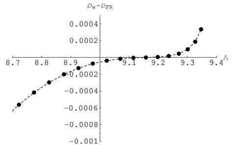
We denote the entropy of the FR branch and that of the warped branch as $S_{\mathrm{FR}}$ and $S_{\mathrm{w}}$, respectively. A difference between $S_{\mathrm{w}}$ and $S_{\mathrm{FR}}$ for various values of the total flux is shown in Fig. 4. It turns out that for $\Phi<32\sqrt{3}\pi^{2}\Lambda^{-3/2}$, or equivalently, for

the warped branch has larger entropy and thus is thermodynamically stable. On the other hand, for $\Phi>32\sqrt{3}\pi^{2}\Lambda^{-3/2}$, or equivalently, for $h^{2}>\frac{\Lambda}{18}$, the FR branch has larger entropy and is thermodynamically stable. At the critical point where two branches merge the solution is marginally stable.

It is worth noting that the thermodynamic stability investigated here agrees with the dynamical stability examined in Sec III. The FR branch has dynamical instability arising from inhomogeneous ($l=2$) excitation when $h^{2}<h^{2}_{\mathrm{c}(l=2)}$, where $h^{2}_{\mathrm{c}(l=2)}$ is given by (27). On the other hand, the warped branch is dynamically unstable for $h^{2}>h^{2}_{\mathrm{c}(l=2)}$. For $p=4$ and $q=4$, the critical value $h^{2}_{\mathrm{c}(l=2)}$ for the dynamical stability agrees with the critical value for the thermodynamic stability given in the right hand side of (47). Therefore, we again see complete agreement between thermodynamic and dynamical stabilities.

References

- [1] P. G. O. Freund and M. A. Rubin, Phys. Lett. B 97, 233 (1980).
- [2] R. Bousso, O. DeWolfe and R. C. Myers, Found. Phys. 33, 297 (2003) [arXiv:hep-th/0205080].
- [3] J. U. Martin, JCAP 0504, 010 (2005) [arXiv:hep-th/0412111].
- [4] T. Torii and T. Shiromizu, Phys. Lett. B 551, 161 (2003) [arXiv:hep-th/0210002].
- [5] C. Krishnan, S. Paban and M. Zanic, JHEP 0505, 045 (2005) [arXiv:hep-th/0503025].
- [6] S. Kinoshita, Phys. Rev. D 76, 124003 (2007) [arXiv:0710.0707 [hep-th]].
- [7] S. S. Gubser and I. Mitra, JHEP 0108, 018 (2001) [arXiv:hep-th/0011127].
- [8] S. S. Gubser and I. Mitra, arXiv:hep-th/0009126.
- [9] H. S. Reall, Phys. Rev. D 64, 044005 (2001) [arXiv:hep-th/0104071].
- [10] T. Prestidge, Phys. Rev. D 61, 084002 (2000) [arXiv:hep-th/9907163].
- [11] J. P. Gregory and S. F. Ross, Phys. Rev. D 64, 124006 (2001) [arXiv:hep-th/0106220].
- [12] V. E. Hubeny and M. Rangamani, JHEP 0205, 027 (2002) [arXiv:hep-th/0202189].
- [13] T. Hirayama, G. Kang and Y. Lee, Phys. Rev. D 67, 024007 (2003) [arXiv:hep-th/0209181].
- [14] U. Miyamoto and H. Kudoh, JHEP 0612, 048 (2006) [arXiv:gr-qc/0609046].
- [15] U. Miyamoto, Phys. Lett. B 659, 380 (2008) [arXiv:0709.1028 [hep-th]].
- [16] Y. Brihaye, T. Delsate and E. Radu, Phys. Lett. B 662, 264 (2008) [arXiv:0710.4034 [hep-th]].
- [17] S. Chen, K. Schleich and D. M. Witt, Phys. Rev. D 78, 126001 (2008) [arXiv:0809.1367 [hep-th]].
- [18] B. Kol, Phys. Rept. 422, 119 (2006) [arXiv:hep-th/0411240].
- [19] T. Harmark, V. Niarchos and N. A. Obers, Class. Quant. Grav. 24, R1 (2007) [arXiv:hep-th/0701022].
- [20] S. Kinoshita, Y. Sendouda and S. Mukohyama, JCAP 0705, 018 (2007) [arXiv:hep-th/0703271].