Transport properties of highly asymmetric hard sphere mixtures
Abstract
The static and dynamic properties of binary mixtures of hard spheres with a diameter ratio of and a mass ratio of are investigated using event driven molecular dynamics. The contact value of the pair correlation functions are found to compare favourably with recently proposed theoretical expressions. The transport coefficients of the mixture, determined from simulation, are compared to the predictions of revised Enskog theory, using both a third-order Sonine expansion and direct simulation Monte Carlo. Overall, Enskog theory provides a fairly good description of the simulation data, with the exception of systems at the smallest mole fraction of larger spheres () examined. A “fines effect” was observed at higher packing fractions, where adding smaller spheres to a system of large spheres decreases the viscosity of the mixture; this effect is not captured by Enskog theory.
pacs
Valid PACS appear hereI Introduction
Excluded volume interactions between molecules play a major role in determining the structure and properties of most fluids and colloidal systems. The hard sphere model, which captures the essence of these interactions, has played a central role in our understanding of the properties of fluids, serving as a starting point of perturbation theories for the description of real fluids [1]. Recently, there has been interest in binary hard sphere mixtures, where the diameters of the two components are very different. These systems serve as models for nanoparticle suspensions and colloid-polymer mixtures. In these systems, an entropically driven depletion force [2, 3] drives the larger particles to cluster. While there have been many studies on the structural (e.g., radial distribution function) and thermodynamic properties (e.g., equation of state) of these mixtures [4, 5, 6, 7, 8, 9, 10, 11, 15, 12, 13, 14], there have been relatively few studies on their dynamical properties.
Much of the previous simulation work for the dynamical properties of binary mixtures has focused on tracer particle studies [16, 17, 18], the velocity auto correlation functions, or the self-diffusion coefficients [19, 20], as these are relatively computationally inexpensive to determine. These studies have revealed that the dynamics of the larger particles deviates significantly from both the theoretical predictions of Brownian particles and of Enskog theory. Lue and Woodcock [8, 10] examined the self-diffusion coefficients of size asymmetric binary mixtures of hard spheres. They found a “fines effect” at high densities, where the addition of smaller spheres enhances the mobility of the larger spheres.
Significantly less data are available for other dynamical properties. Easteal and Woolf [21] have investigated the tracer diffusion coefficient for binary hard sphere mixtures. They observe an inverse isotopic mass effect, where heavier tracer particles diffuse faster beyond a certain solvent density than lighter tracer particles. Due to the computational cost of simulating highly size asymmetric systems, past studies have focused on small size disparity and/or moderate mole fractions of colloidal particles.
Erpenbeck [22, 23, 24] provided the first complete transport study, comparing predictions from Enskog theory and molecular dynamics results for binary hard sphere mixtures approximating a Helium-Xenon gas mixture. The mutual diffusion, thermal diffusion, thermal conductivity and shear viscosity are given over a range of state points. Enskog theory was found to provide a fairly good description of the transport properties for the conditions studied. Yeganegi and Zolfaghari [25] have investigated the thermal diffusion coefficient of binary hard spheres (for moderate size ratios) using non-equilibrium molecular dynamics. They observe a minimum in the thermal diffusion with density and good agreement with Enskog theory. Recently, Bastea [26] has investigated the viscosity and thermal conductivity of highly asymmetric “soft-sphere” mixtures at very low volume fractions of the larger spheres. Enskog theory was only able to qualitatively describe the results in that study.
In the present work, we perform event driven molecular dynamics simulations to study the static and transport properties of binary hard sphere mixtures with a diameter ratio of 0.1 and a mass ratio of 0.001. One of the motivations of this work is to further explore the “fines effect” revealed in these systems in a previous study by Lue and Woodcock [10]. Another aim of this work is to quantitatively test the predictive ability of the revised Enskog theory [27] for these binary hard sphere systems over a broad range of conditions. The remainder of this paper is organized as follows. Details of the hard sphere mixture model and the relation of the transport coefficients to the microscopic dynamics of the system are discussed in Section II. The details of the molecular dynamics calculations and the direct simulation Monte Carlo solution of the Enskog equation are provided in Section III. The simulation data for the static and the transport properties of the binary hard sphere mixtures are presented in Section IV, and the results are compared against the predictions of the Enskog theory. Finally, the main findings of this work are summarized in Section V.
II Theoretical background
We consider systems consisting of additive hard spheres with differing diameters and masses. Spheres of type have a diameter and a mass . The spheres are not permitted to overlap, and so the interaction potential between a sphere of type and a sphere of type is given by
where is the distance between the centers of the two spheres, and . Due to the simple nature of this interaction potential, all properties of hard sphere mixtures have a trivial dependence on the temperature.
One major advantage of the hard sphere model is the simplicity of its dynamics. The dynamics of hard sphere systems is driven by collisions between spheres. Between collisions, the spheres travel at constant velocity. The solution of the trajectory of the system then reduces to determining the sequence of collisions between the spheres. These collisions alter the velocities of the spheres but conserve their energy and momentum. After a collision between a sphere of type and a sphere of type , the velocities of the spheres become and
| (3) |
where and are the velocities of the spheres immediately before collision, is a unit vector pointing from the center of sphere to the center of sphere , is their relative velocity, and is the reduced mass.
II.1 Static properties
The pair correlation functions give an indication of the average local environment of the particles in a system. For hard sphere systems, the values of the pair correlation functions at contact play an important role. In particular, they are directly related to the collision rates between the spheres:
| (4) |
where is the number density of spheres of type , , is the Boltzmann constant, is the absolute temperature, and is the mean time between which a sphere of type undergoes collisions with a sphere of type . The quantity can be calculated from the number of - collisions that occur in a simulation of duration
| (5) |
where is the number of spheres of type in the system. An advantage of molecular dynamics simulations over Monte Carlo simulations is that the contact values of the pair correlation functions can be directly calculated from the times and does not require the extrapolation of the pair correlation to contact.
The contact values of the pair correlation functions are also directly related to the equation of state of the hard sphere system:
| (6) |
where is the system pressure, is the total number density of spheres, is the mole fraction of spheres of type , and the lowercase Latin indexes run over all species (i.e. and for a binary mixture) present in the system.
Due to the fundamental importance of the contact values of the pair correlation functions for hard sphere systems, there have been many efforts to develop expressions to describe them [5, 6, 9, 28]. One of the most popular is the Boublik-Mansoori-Carnahan-Starling (BMCSL) equation of state [29, 30], which is an interpolation between the virial and compressibility expressions of the Percus-Yevick theory [31]. This is given by
| (7) |
where is defined by
| (8) |
Note that the solid fraction occupied by the spheres is given by .
The BMCSL equation yields predictions that are generally in good agreement with simulation data for hard sphere mixtures over a broad range of diameters and compositions [4]. However, for highly size asymmetric binary systems at small mole fractions of the larger spheres (often referred to as the colloidal limit), the BMCSL significantly underpredicts the contact value of the pair correlation function between the larger spheres, as compared to simulation results [4, 8, 32].
Recently, there have been several efforts to correct this. Viduna and Smith [33, 34] have suggested a new expression, based on an empirical equation of state
| (9) |
This compact expression appears to compare well with simulation results. In the case of binary hard sphere mixtures, Henderson et al. [11] have suggested further modifications to the BMCSL and VS equations so that the contact value of the pair correlation function between the larger spheres yield the correct limiting behavior as the diameters of the larger spheres become infinite [32]. Their expressions for the pair correlation functions (which we denote as HC2) are given by
| (10) | ||||
| (11) | ||||
| (12) |
where refers to the larger spheres, refers to the smaller spheres, is the diameter ratio, and .
II.2 Calculation of transport coefficients
In the continuum description of fluids [35], balance equations are typically used to relate the conserved properties of the system (e.g., energy, momentum, and mass) to their fluxes. To close these equations, constitutive relations are required. These relations link the diffusive fluxes to gradients in the thermodynamic properties of the system. Transport coefficients are defined through the assumption that the diffusive fluxes depend linearly on the thermodynamic driving forces, which are gradients of local thermodynamic properties of the system.
There are several possible choices [35] for the thermodynamic forces and the diffusive fluxes . For NVE molecular dynamics simulations, the most convenient [22] choice is the “mainstream” (or “unprimed” [35, 22]) definition of the fluxes. These are defined as
| (13a) | ||||||
| (13b) | ||||||
where is the chemical potential, and is the diffusive flux of species , is the energy flux, is the thermal conductivity, is the mutual diffusion coefficient, and is the thermal diffusivity. The transport coefficients are defined through Eqs. (13).
The relationship between stress tensor and the strain rate in the fluid is defined in the standard manner:
| (14) |
where is the shear viscosity, is the bulk viscosity, and is the streamline velocity of the fluid. The quantity represents the unit matrix, and the superscript T indicates the transpose of a matrix.
The Onsager reciprocity relations ( and ), combined with the requirement that (due to the definition of the diffusive flux) which implies , reduce the number of independent transport coefficients to , , , , and . In the following section, we discuss how these transport coefficients can be determined from equilibrium molecular dynamics simulations.
II.3 Einstein forms of the Green-Kubo relations
The Green-Kubo formulas relate the time correlation functions of the microscopic fluxes directly to the transport coefficients [1]. However, the Green-Kubo relations are an unpopular method for obtaining the transport coefficients from molecular dynamics simulations, as they require long simulation times to obtain good statistics. This is not a significant issue in hard sphere systems, as long simulation times are more easily accessible. For systems with particles interacting with discontinuous potentials, the Einstein form of the Green-Kubo relations must be used, due to the impulsive nature of the interaction potential. The full derivation of the these formulas are already available [22, 1], and, therefore, only the final expressions are presented here for completeness.
The Einstein relations have the general form
| (15) |
where is a time dependent transport coefficient, is the volume of the system, and and are displacement functions corresponding to time integrals of the microscopic fluxes. The displacement functions for a system with zero total momentum in the microcanonical ensemble are given in Table 1. The pair of displacement functions that correspond to each of the transport coefficients are summarized in Table 2. In hydrodynamic regime, the transport coefficients are given by the infinite time limit of Eq. (15)
| (16) |
A sample of reduced correlators for a single molecular dynamics simulation run is plotted in Fig. 1. The function typically displays transient behavior for short times before changing to the linear, long-time regime. All the transport properties, with the exception of the bulk viscosity, rapidly transition to the linear regime within a few mean free times. The bulk viscosity, however, only slowly approaches the linear regime, and, consequently, the limiting values are difficult to extract. As a result, we do not present data for the bulk viscosity.
A time correlation function of a finite sized simulation is only representative of a bulk system for a limited duration. Beyond the time a sound wave takes to traverse the simulation box, the system size begins to affect the correlation function. The sound wave traversal time is determined directly from the speed of sound, . For a hard sphere system the speed of sound is given by
| (17) |
where is the compressibility factor, and is the mean particle mass. The HC2 equation of state (see Eqs. (6), (10), (11), and (12)) is used to estimate the speed of sound, via Eq. (17). Data for the time correlation functions are only collected for a duration of time shorter than the sound wave traversal time.
II.4 Enskog theory predictions for the transport coefficients
Revised Enskog theory (RET) [27, 36, 37, 38] is an extension of the highly successful Enskog theory to mixtures. This is the most widely applied kinetic theory of moderately dense fluids. In the Enskog approximation, all pre-collision correlations between particles are ignored, save for a single static structural correlation function. In a homogeneous system, this reduces to the values of the various pair correlation functions at contact, which govern the collision rates. Given these as input, Enskog theory yields predictions for the transport properties through the Chapman-Enskog expansion [39].
The standard method to solve to the Enskog equation is to expand the one-particle distribution function in a series of Sonine polynomials. Erpenbeck [22] has compiled the (corrected) Enskog expressions for all transport properties, excluding the bulk viscosity, of hard sphere mixtures. These expressions have been combined with the table of integrals given by Ferziger and Kaper [40] and a linear equation solver to evaluate Enskog theory to the third order in the Sonine expansion. We present results calculated from the BMCSL and HC2 equations to determine the effect of improved values for on the predictions of the transport properties.
II.5 DSMC solution of the Enskog equation
Another method for obtaining solutions to the Enskog equations is through the use of the direct simulation Monte Carlo (DSMC) method. This technique was originally developed for the Boltzmann equation but has recently been extended to the Enskog equation [41, 42, 43]. In this work, DSMC of the Enskog equation, in the style of Bird’s NTC method [44], is used to provide results. In this approach, the velocity distribution of each species is approximated using a set of samples
| (18) |
where is the number of samples of the velocity distribution of species . For simplicity, in the following expressions we assume each sample represents a single sphere. Other choices are possible; however, the difference merely affects the relative sample collision testing rates and time scale of the simulation.
The probability that a sample of species undergoes a collision event with species after a time step is [45]
| (19) |
where is a randomly chosen sample from species , is a randomly chosen relative orientation between the samples on collision, is the relative velocity, and is the Heaviside step function. The time step describes the rate at which samples in species are tested for collisions with a sample of species . For a DSMC calculation of a binary mixture, there are four rates, one for each pairing of the species (, , , and ).
The simplest DSMC algorithm proceeds by incrementing time to the next test for collisions between species and . Each sample of species is tested for an event with another sample , which is randomly selected. A collision is executed with a probability given by Eq. (19). This collision only affects sample and not the collision partner . This method is simple but inefficient because properties that are conserved on collision (e.g., momentum and energy) are only conserved on average. In addition, all samples in species are tested at each time step, which is computationally expensive, even though is selected to yield only a few events per time step.
An improved algorithm, based on Bird’s NTC method, executes symmetric species-species collision events simultaneously, and, therefore, there are three independent test rates for the binary system (, , and ). For a given time step, we assume there are a maximum of events that may occur for each species; the quantity is the maximum observed value of , which is updated, if required, during the course of a simulation. pairs of and samples are randomly selected at each time step. The probability of collision is then scaled to
| (20) |
where is the Kronecker delta. If the collision is accepted, then the velocities of both samples are updated according to the collision rule (see Eq. (3)). This conserves energy and momentum at all times and greatly improves the statistics of the simulation. Like Enskog theory, the DSMC calculations require as input, however, DSMC requires no polynomial expansion to make the problem tractable.
The transport coefficients are obtained through the use of the appropriate time correlation functions, as in the full molecular dynamics simulations (see Section II.2). DSMC provides an attractive method of numerically solving a kinetic equation, especially as computing power increases. Its results are still, however, limited by the approximations of the underlying kinetic equation.
III Simulation details
In this work, we examine the static and transport properties of highly asymmetric binary hard sphere mixtures. The larger spheres have a diameter and mass , and the smaller spheres have a diameter and mass . We consider systems with and , consistent with particles of the same density.
Discrete potentials, such as the hard sphere model, have an important advantage over more complex “soft” potentials. Between collisions the spheres or molecules experience no forces and travel on ballistic trajectories. The dynamics can be solved analytically, and the integration of the equations of motion is processed as a sequence of events. Current event driven molecular dynamics algorithms are now quite advanced and allow the simulation of large systems for the long times required to extract accurate transport properties.
III.1 MD Simulations
The basic event driven algorithm used in this work to perform the molecular dynamics simulations is fundamentally the same as the one originally described by Alder and Wainwright [46]. Neighbor lists and the delayed states algorithm [47] are included to optimize the calculations. These methods are combined with a new bounded priority queue, suggested by Paul [48], to remove the system size dependence of sorting the event queue. Finally, the interactions between the largest spheres are removed from the neighbor list and processed separately [12] to allow the use of a smaller cell size and reduced number of collision tests. This removal is restricted to low mole fractions of the larger spheres as the overhead of these removed interactions is of order in the number of large spheres.
A total of spheres in a cubic box of volume with standard periodic boundary conditions were used in all the simulations. The volume of the system and the relative number of large and small spheres (i.e., and ) were adjusted to obtain the required packing fraction and composition, respectively. For each of the systems examined, the initial configurations were equilibrated over a period of collisions and then run for trajectories of collisions to collect the collision statistics and time correlation functions.
The time correlation functions for the various transport properties were collected over approximately intervals of a mean free time, using the start time averaging method [49]. The last values of the correlator were fitted to a line to extract the long time limit of the transport coefficient.
III.2 DSMC simulations
DSMC simulations were performed using a total of samples of the velocity distribution. Each of the simulations was initially equilibrated for collisions. The time correlation functions were then collected over separate trajectories, each consisting of collisions, using intervals of a mean free time. The statistical uncertainty of the shorter DSMC calculations are smaller than the uncertainties of the MD simulations because Enskog theory neglects dynamical correlations.
IV Results and discussion
In this section, we present the results of the molecular dynamics simulations for the contact value of the pair correlation functions and the transport coefficients of binary hard sphere mixtures. A comparison of the predictions of the revised Enskog theory is also provided. All quantities are reported in reduced units, where the unit of mass is , the unit of length is , and the unit of energy is .
IV.1 Static properties
The variation of the pressure of the binary hard sphere mixtures with packing fraction and composition is shown in Fig. 2. The symbols are the data from the molecular dynamics simulations, and the lines are the predictions of the BMCSL (solid) and HC2 (dotted) equations of state. These equations of state provide an excellent description of the simulation data, with the exception of the very highest packing fractions where they overpredict the pressure. These deviations, however, are due to the onset of freezing of the larger spheres; the single component hard sphere fluid begins to freeze at a packing fraction of [50].
The contact values of the , , and pair correlation functions are plotted in Fig. 3 as a function of the total volume fraction of spheres for different mole fractions of the larger spheres . The simulation results for are well described by the BMCSL theory. This is in agreement with previous simulation studies of binary hard spheres mixtures [8, 13]. The VS predictions (not shown) provide equally accurate predictions for .
The BMCSL predictions for lie above the simulation results at high density for the lowest mole fraction studied. The HC2 predictions are higher still, however, the error is within a few percent. The corrections of Henderson et al. [11] to are small for the systems studied. The VS predictions (not shown) lie between the HC2 and the BMCSL results
For the contact value of pair correlation function between the larger spheres, the BMCSL predictions fall significantly below the simulation results at high density for the lowest mole fraction studied. The HC2 predictions are exceptionally accurate, even for the smallest mole fractions of the larger spheres. This is due to the success of the underlying VS equation (not shown), which give results that are nearly indistinguishable from the HC2 equation. At , for the system decreases significantly. This also occurs in the system at a higher packing fraction of . It appears that the larger component has frozen while the smaller spheres remain fluid.
Overall, the HC2 expression is accurate and provides excellent estimates for the contact values of the pair correlation functions for all the conditions studied in this work.
IV.2 Thermal conductivity
The thermal conductivity of the binary hard sphere mixtures is plotted in Fig. 4a with respect to the packing fraction and in Fig. 4b with respect to the pressure. The molecular dynamics simulation data are given by the filled symbols. The crosses are molecular simulation data for single component hard spheres, taken from Ref. 51. For single component hard sphere systems, the thermal conductivity increases with increasing packing fraction and pressure. The initial addition of smaller spheres to a system of larger spheres (i.e. decreasing ) significantly increases the thermal conductivity of the mixture. At the same packing fraction, a system with a lower mole fraction of larger spheres will have many more particles than a system with a higher mole fraction of larger spheres. These additional particles enhance the ability of system to transport energy. With the addition of smaller spheres to the large sphere system, we observe that the thermal conductivity no longer increases monotonically with the packing fraction (or the pressure). Rather, the thermal conductivity initially decreases with increasing packing fraction down to a minimum value, and then it increases. The packing fraction at the minimum increases as the fraction of smaller spheres increases.
Interestingly, at packing fractions below , the thermal conductivity of pure spheres (i.e., ) is lower than the thermal conductivity for the system, while for it is higher. This implies that at sufficiently low packing fraction (or pressure) the thermal conductivity of the system must have a maximum with respect to . Physically, this would correspond to a situation where the addition of larger spheres to a fluid of smaller hard spheres would enhance its thermal conductivity.
The solid lines in Fig. 4 are the predictions of Enskog theory within the third order Sonine approximation with the BMCSL expressions for the collision rates, while the dotted lines are the third order Enskog predictions with the HC2 expressions. The difference between using the BMCSL and HC2 expressions in Enskog theory is negligible, as the collisional contribution to the thermal conductivity is dominated by the and interactions (see Figs. 3b and c). The open symbols in Fig. 4 are from DSMC calculations using the HC2 expressions for the collision rates. These results are nearly identical to the third order Sonine approximation, indicating the accuracy of the approximation and validating the DSMC code.
The simulation results are well described by Enskog theory for the pure hard sphere systems (i.e. and ), as well as for mixtures with relatively high mole fractions of the larger spheres (). At high packing fractions, the Enskog predictions deviate slightly for the case ; however, this occurs at the conditions where component appears to freeze (see Fig. 3a), and the BMCSL and HC2 expressions for are not applicable for solid phases.
For , Enskog theory significantly underpredicts the thermal conductivity of the system. This deviation may be related to the enhanced mobility of the system due to the fines effect [10] and is a result of a dynamic process not captured by Enskog theory. Note, however, that Enskog theory provides good predictions for the thermal conductivity of one component hard sphere systems [51], so one expects that for vanishing amounts of the larger spheres (i.e. the limit where ), Enskog theory should again provide a fairly good description of the simulation data.
IV.3 Shear viscosity
The shear viscosity is plotted in Fig. 5. The viscosity of all the mixtures increases monotonically with the packing fraction of the spheres and the pressure of the system (see Fig. 5a-c). Unlike for the thermal conductivity, the Enskog theory predictions for the shear viscosity using the HC2 expression for the collision rates noticeably differ from the BMCSL results (see Fig. 5a); however, this only occurs in regions where Enskog theory poorly describes the simulation results (see Fig. 5b and c). Enskog theory captures the low density behavior of the viscosity quite well. For single component hard sphere systems, Enskog theory is known to underpredict the viscosity at high densities [52], due to its inability to account for correlated collisions resulting from the caging of spheres at these conditions. For the binary hard sphere mixtures that we study here, the Enskog theory underpredicts the viscosity, in general. However, the case is an exception, where Enskog theory actually overpredicts the viscosity at high packing fractions.
An interesting “fines” effect occurs in the viscosity of these systems. At low overall packing fractions (or pressures), the addition of smaller spheres to a system of larger spheres (i.e. decreasing ) increases the viscosity of the system. However, above a packing fraction of about , the curves for the viscosity crossover, and the addition of smaller spheres to a system of larger spheres decreases the viscosity of the system. This is highlighted in Fig. 5d where the viscosity is almost independent of composition at a packing fraction of . The “fines” effect is not captured by Enskog theory, which indicates its origin is in dynamical correlations between particles. In these systems, the presence of the smaller spheres leads to an attractive depletion force [2, 3] between the larger spheres, which is entropically driven. This force may disrupt the caging of larger spheres [10] by forcing them into closer contact, thereby creating a more open network and increasing the mobility of both species.
IV.4 Thermal diffusion coefficient
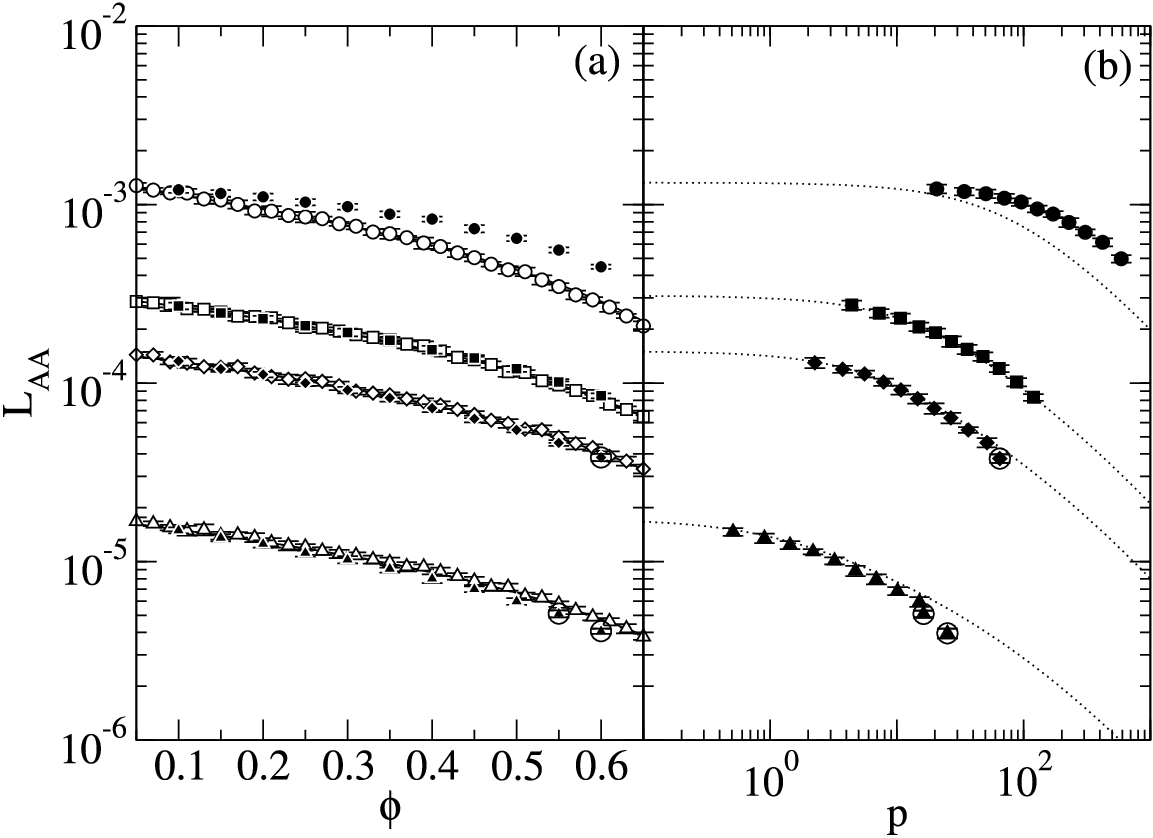
Figure 6 presents the thermal diffusivity of the larger spheres over a range of packing fractions and pressures. Because is negative, the larger species tends to move towards regions of higher temperature. Increasing the packing fraction, the pressure, or the fraction of larger spheres in the system decreases the magnitude of the thermal diffusivity. This general trend is in agreement with previous NEMD simulations [25].
The use of the HC2 expressions with Enskog theory offers no significant improvement on the BMCSL predictions, again due to the dominance of the small spheres in the energy transport. Enskog theory is in quantitative agreement with the simulation data over a broad range of conditions examined in this work. However, the main exception is for the composition , where it substantially underpredicts the at the higher packing fractions.
IV.5 Mutual diffusion coefficient
The mutual diffusion coefficient of the binary hard sphere mixtures is plotted in Fig. 7. The mutual diffusion coefficient behaves similarly to the thermal diffusivity. The displacement functions required to calculated this transport coefficient contain no potential terms, and therefore, they do not contain a collisional component of the flux (see Tables 1 and 2). Consequently, Enskog theory performs equally well with HC2 or BMCSL contact radial distribution values. Similar to the results for the thermal diffusivity, Enskog theory is in quantitative agreement with the simulation data over most of the conditions examined, with the exception of the systems, where it significantly underpredicts the diffusion coefficient.
V Conclusions
In this work, we examined the properties of binary mixtures of hard spheres with a diameter ratio of and a mass ratio of . The BMCSL equation of state is able to accurately describe the pressure for all the conditions that we investigated where the system did not freeze. However, it underpredicts the value of and , especially at high packing fractions and low mole fractions of the larger spheres. The recently developed HC2 equation, however, is able to quantitatively predict these quantities.
Enskog theory provides fairly accurate predictions for the transport coefficients of the systems that we studied in this work. The third order Sonine approximation and the DSMC results agree well with one another, both validating the DSMC code and demonstrating that the third order solution is sufficiently accurate over the conditions studied. At low mole fractions of the larger hard spheres, Enskog theory fails to capture the behavior of the transport properties, especially the shear viscosity. This may be due to the increased correlations in the collisions between the larger spheres caused by the depletion forces due to the presence of the smaller spheres.
DSMC provides a speed benefit over traditional molecular dynamics simulations where large size asymmetries and low mole fractions are computationally expensive. Unfortunately, this is where Enskog theory begins to break down in predicting the transport properties of the fluid. Extension of DSMC to other kinetic theories, such as ring theory, is necessary to capture this behavior, however, these techniques are yet to be developed.
We find a “fines” effect where the addition of smaller spheres to a larger hard sphere fluid decreases the viscosity of the system, which occurs at packing fractions greater than about 0.4. This effect is not captured by Enskog theory. With the addition of fines, the thermal conductivity of the mixture no longer monotonically increases with the packing fraction but instead initially decreases with increasing packing fraction to a minimum value and then increases. In addition, at low to moderate packing fractions, there is a region in where the thermal conductivity of the mixture is higher than thermal conductivity of either pure species.
Acknowledgements.
MN Bannerman acknowledges support from an EPSRC DTA.References
- [1] J. P. Hansen and I. R. McDonald, Theory of Simple Liquids (Academic Press, London, 1986), 2nd ed.
- [2] F. Oosawa and S. Asakura, J. Chem. Phys. 22, 1255 (1954).
- [3] A. Vrij, Pure Appl. Chem. 48, 471 (1976).
- [4] G. Jackson, J. S. Rowlinson, and F. van Swol, J. Phys. Chem 91, 4907 (1987).
- [5] D. H. L. Yau, K.-Y. Chan, and D. Henderson, Mol. Phys. 88, 1237 (1996).
- [6] D. H. L. Yau, K.-Y. Chan, and D. Henderson, Mol. Phys. 91, 1137 (1997).
- [7] D. Henderson, D. H. L. Yau, and C. Kwong-Yu, Mol. Phys. 88, 1237 (1996).
- [8] L. Lue and L. V. Woodcock, Mol. Phys. 96, 1435 (1999).
- [9] K.-Y. Chan and D. Henderson, Mol. Phys. 98, 1005 (2000).
- [10] L. Lue and L. V. Woodcock, Int. J. Thermophys. 23, 937 (2002).
- [11] D. Henderson, A. Trokhymchuk, L. V. Woodcock, and C. Kwong-Yu, Mol. Phys. 103, 667 (2005).
- [12] A. Vrabecz and G. Tóth, Mol. Phys. 104, 1843 (2006).
- [13] M. Alawneh and D. Henderson, Mol. Phys. 106, 607 (2008a).
- [14] M. Alawneh and D. Henderson, Mol. Phys. 106, 2407 (2008b).
- [15] A. Santos and M. L. López de Haro, J. Chem. Phys. 123, 234512 (2005).
- [16] P. T. Herman and B. J. Alder, J. Chem. Phys. 56, 987 (1972).
- [17] G. Subramanian, D. Levitt, and H. T. Davis, J. Chem. Phys. 60, 591 (1974).
- [18] B. J. Alder, W. E. Alley, and J. H. Dymond, J. Chem. Phys. 61, 1415 (1974).
- [19] V. Y. Rudyak, G. V. Kharlamov, and A. A. Belkin, Tech. Phys. Let. 26, 553 (2000).
- [20] V. Y. Rudyak, G. V. Kharlamov, and A. A. Belkin, High Temp. 39, 264 (2001).
- [21] A. J. Easteal and L. A. Woolf, Chem. Phys. Lett. 167, 329 (1990).
- [22] J. J. Erpenbeck, Phys. Rev. A 39, 4718 (1989).
- [23] J. J. Erpenbeck, Phys. Rev. A 45, 2298 (1992).
- [24] J. J. Erpenbeck, Phys. Rev. E 48, 223 (1993).
- [25] S. Yeganegi and M. Zolfaghari, Fluid Phase Equilibria 243, 161 (2006), ISSN 0378-3812.
- [26] S. Bastea, Phys. Rev. E 75, 031201 (2007).
- [27] M. López de Haro, E. G. D. Cohen, and J. M. Kincaid, J. Chem. Phys. 78, 2746 (1983).
- [28] D. V. Matyushov and B. Ladanyi, J. Chem. Phys. 107, 5815 (1997).
- [29] T. Boublik, J. Chem. Phys. 53, 471 (1970).
- [30] G. A. Mansoori, N. F. Carnahan, K. E. Starling, and T. W. Leland, J. Chem. Phys. 54, 1523 (1971).
- [31] J. K. Percus and G. J. Yevick, Phys. Rev. 110, 1 (1958).
- [32] R. Roth, R. Evans, and S. Dietrich, Phys. Rev. E 57, 6785 (2000).
- [33] D. Viduna and W. R. Smith, J. Chem. Phys. 117, 1214 (2002a).
- [34] D. Viduna and W. R. Smith, Mol. Phys. 100, 2903 (2002b).
- [35] S. de Groot and P. Mazur, Non-Equilibrium Thermodynamics (Dover, New York, 1984).
- [36] J. M. Kincaid, M. López de Haro, and E. G. D. Cohen, J. Chem. Phys. 79, 4509 (1983).
- [37] M. L. López de Haro and E. G. D. Cohen, J. Chem. Phys. 80, 408 (1984).
- [38] J. M. Kincaid, E. G. D. Cohen, and M. López de Haro, J. Chem. Phys. 86, 963 (1987).
- [39] S. Chapman and T. G. Cowling, The Mathematical Theory of Non-Uniform Gases (Cambridge, Cambridge, 1970), 3rd ed.
- [40] J. H. Ferziger and H. G. Kaper, Mathematical Theory of Transport Processes in Gases (North-Holland, London, 1972).
- [41] J. M. Montanero and A. Santos, Phys. Rev. E 54, 438 (1996).
- [42] J. M. Montanero and A. Santos, Phys. Fluids 9, 2057 (1997).
- [43] A. Frezzotti, Phys. Fluids 9, 1329 (1997).
- [44] G. A. Bird, Molecular gas dynamics and the direct simulation of gas flows (Oxford Science, 1994).
- [45] M. A. Hopkins and H. H. Shen, J. Fluid Mech. 244, 477 (1992).
- [46] B. J. Alder and T. E. Wainwright, J. Chem. Phys. 31, 459 (1959).
- [47] M. Marin, D. Risso, and P. Cordero, J. Comput. Phys. 109, 306 (1993).
- [48] G. Paul, J. Comp. Phys. 221, 615 (2007).
- [49] J. M. Haile, Molecular Dynamics Simulation - Elementary Methods (Wiley-Interscience, New York, 1997).
- [50] W. G. Hoover and F. H. Ree, J. Chem. Phys. 49, 3609 (1968).
- [51] L. Lue, J. Chem. Phys. 122, 044513 (2005).
- [52] L. Lue and M. Bishop, Phys. Rev. E 74, 021201 (2006).