For the 9th conference of Japanese Society for Artificial Intelligence, Special Interest Group on Data Mining and Statistical Mathematics
(JSAI SIG-DMSM) in Kyoto 2009, March 3,4.

We introduce a probabilistic model considered in this paper, MRF of binary states with pairwise interactions. Let $G:=(V,E)$ be a connected undirected graph, where $V=\{1,\ldots,N\}$ is a set of nodes and $E\subset\{(i,j);1\leq i<j\leq N\}$ is a set of undirected edges. We abbreviate undirected edges $(i,j)$ to $ij=ji$. Each node $i\in V$ is associated with a binary space $\chi_{i}=\{\pm 1\}$. We make a set of directed edges from $E$: $\vec{E}=\{(i,j),(j,i);(i,j)\in E\}$. The neighbors of $i$ is denoted by $N(i)\subset V$, and $d_{i}=|N(i)|$ is called the degree of $i$. A joint probability distribution on the graph $G$ is given by the form:

where $\psi_{ij}(x_{i},x_{j}):\chi_{i}\times\chi_{j}\rightarrow\mathbb{R}_{>0}$ and $\phi_{i}:\chi_{i}\rightarrow\mathbb{R}_{>0}$ are positive functions called compatibility functions. The normalization factor $Z$ is called the partition function. A set of random variables which has a probability distribution in the form of (1) is called a Markov random field (MRF) or an undirected graphical model on the graph $G$.

Without loss of generality, univariate compatibility functions $\phi_{i}$ can be neglected because they can be included in bivariate compatibility functions $\psi_{ij}$. This operation does not affect the Bethe approximation and the LBP algorithm given below; we assume it as per the following.

The LBP algorithm computes the Bethe approximation of the partition function and the marginal distribution of each node with the message passing method [9, 2, 3]. This algorithm is summarized as follows.

1. 1.

   Initialization:
   For all $(j,i)\in\vec{E}$, the message from $i$ to $j$ is a vector $m_{(j,i)}^{0}\in\large{\mathbb{R}}^{2}$. Initialize as

   $\displaystyle m_{(j,i)}^{0}(x_{j})=1\quad\forall x_{j}\in\chi_{j}.$

   (2)

2. 2.

   Message Passing:
   For each $t=0,1,\ldots$, update the messages by

   $$m^{t+1}_{(j,i)}(x_{j})=\omega\sum_{x_{i}\in\chi_{i}}\hskip-2.84526pt\psi_{ji}(x_{j},x_{i})\hskip-5.69054pt\prod_{k\in N(i)\backslash\{j\}}\hskip-11.38109ptm^{t}_{(i,k)}(x_{i}),$$

   (3)

   until it converges. Finally we obtain $\{m^{*}_{(j,i)}\}$.

3. 3.

   Approximated marginals and the partition function are computed by the following formulas:

   $$\hskip-65.44133ptb_{i}(x_{i}):=\omega\prod_{j\in N(i)}m^{*}_{(i,j)}(x_{i}),$$

   (4)

   $$b_{ji}(x_{j},x_{i}):=\omega\psi_{ji}(x_{j},x_{i})\hskip-5.69054pt\prod_{k\in N(j)\backslash\{i\}}\hskip-5.69054ptm^{*}_{(j,k)}(x_{j})\\ \prod_{k^{\prime}\in N(i)\backslash\{j\}}\hskip-5.69054ptm^{*}_{(i,k^{\prime})}(x_{i}),$$

   (5)

   $$\log Z_{B}:=\sum_{ji\in{E}}\sum_{x_{j},x_{i}}b_{ji}(x_{j},x_{i})\log\psi_{ji}(x_{j},x_{i})\\ -\sum_{ji\in{E}}\sum_{x_{j}x_{i}}b_{ji}(x_{j},x_{i})\log b_{ji}(x_{j},x_{i})\\ +\sum_{i\in V}(d_{i}-1)\sum_{x_{i}}b_{i}(x_{i})\log b_{i}(x_{i}),$$

   (6)

   where $\omega$ are appropriate normalization constants, $b_{i}$ are called beliefs, and $Z_{B}$ is called the Bethe approximation of the partition function.

In step 2, there is ambiguity as to the order of updating the messages. We do not specify the order, because the fixed points of LBP algorithm do not depend on its choice.

We normalize as $\sum_{x_{i},x_{j}}b_{ji}(x_{j},x_{i})=\sum_{x_{i}}b_{i}(x_{i})=1$, so that the relation $\sum_{x_{i}}b_{ji}(x_{j},x_{i})=b_{j}(x_{j})$ is always satisfied for all $ij\in E$.

First, we prove the following identity which plays a key role in our derivation. We define a set of polynomials $\{f_{n}(x)\}_{n=0}^{\infty}$ inductively by the relations $f_{0}(x)=1,f_{1}(x)=0$ and $f_{n+1}(x)=xf_{n}(x)+f_{n-1}(x)$. This polynomials are transformations of the Chebyshev polynomials of the second kind.

Secondly, we give a relation between the true partition function and the Bethe approximation.

Finally, we give the loop series expansion formula of the partition function [1, 7, 8].

Before accomplishing the proof, let us consider the meaning of the theorem. Equation (12) states that $\gamma_{i}$ is related to the bias of the approximated marginal $b_{i}(x_{i})$, and $\gamma_{i}=0$ if and only if $b_{i}(1)=b_{i}(-1)$. Equation (13) states that $\beta_{ij}$ is related to the correlation by $b_{ij}$. It is easy to see that $|\beta_{ij}|\leq 1$ and $\beta_{ij}=0$ if and only if $b_{ij}(x_{i},x_{j})=b_{i}(x_{i})b_{j}(x_{j})$.

The definitions and properties of these quantities $\beta_{ij}$ and $\gamma_{i}$, in the context of message passing procedures, are found in [1].

In (14), the summation runs over all subsets of $E$ including $s=\phi$. As $f_{1}(x)=0$, $s$ makes a contribution to the sum only if $s$ does not have a node of degree one in $s$. Such a subgraph $s$ is called a generalized loop [7, 8] or a closed graph [12, 13]. In the case that $G$ is a tree, there is no generalized loops, therefore $Z=Z_{B}$. This is an alternative proof of the well-known fact [9].

If $\beta_{ij}$ an $\gamma_{i}$ are sufficiently small, the first term $r(\phi)=1$ is mainly contribute to the sum, and $Z_{B}$ is close to $Z$.

In this subsection, we head for proving theorem 3. We define a set of polynomials $\{g_{n}(x)\}_{n=0}^{\infty}$ inductively by the relations $g_{0}(x)=x,g_{1}(x)=-2$ and $g_{n+1}(x)=xg_{n}(x)+g_{n-1}(x)$. This set of polynomials is a transformation of the Chebyshev polynomials of the first kind. We introduce the following lemma which is a modification of theorem 1.

A problem of finding an assignment that maximize the marginal probability $p_{1}$ is called maximum marginal assignment problem. This problem is especially important in the application of error correcting code [4, 5]. It is known that if the graph has one cycle and the concerning node $1\in V$ is on the unique cycle, then the assignment that maximize the belief $b_{1}$ gives the exact assignment [10]. With theorem 3, this fact is easily deduced as follows [1].

We append a comment on theorem 3. In the sum of (22), the contribution of $s=\phi$ is equal to $g_{0}(\gamma_{1})=\gamma_{1}$: this is proportional to $b_{1}(+)-b_{1}(-1)$. The assignment that maximize the belief $b_{1}$ can be regarded as the Bethe approximation in the view point of theorem 3.

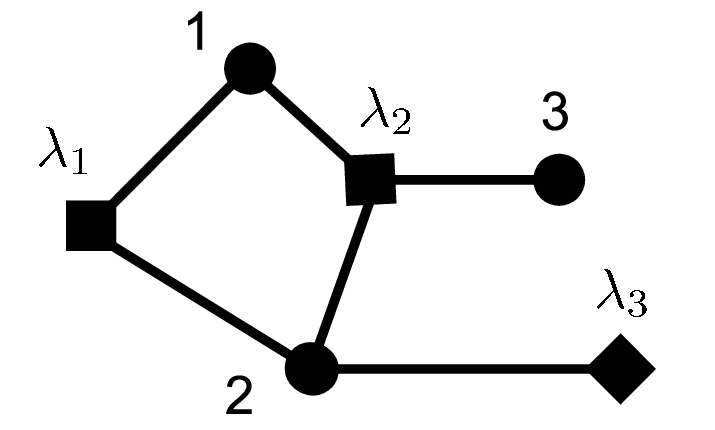
Let $H:=(V,F)$ be a hypergraph, that is, $V=\{1,\ldots,N\}$ is a set of nodes and $F\subset 2^{V}$ is a set of hyperedges. A hypergraph $H$ is represented by a bipartite graph $G_{H}=(V_{H},E_{H})$. Each type of node corresponds to elements of $V$ and $F$; the first type is called variable node and the second type is called factor node. For example, see figure 4. In this example, the hypergraph $H=(V,F)$ is given by $V=\{1,2,3\}$ and $F=\{\lambda_{1},\lambda_{2},\lambda_{3}\}$ ,where $\lambda_{1}=\{1,2\},\lambda_{2}=\{1,2,3\}$ and $\lambda_{3}=\{2\}$.

The joint probability distribution is given by the following form:

where $x_{\lambda}=\{x_{i}\}_{i\in\lambda}$. If each hyperedge $\lambda\in F$ consists of a pair of nodes, this class of probability distributions reduces to the pairwise MRF model.

For a node $i\in V$ and a hyperedge $\lambda\in F$ which satisfy $i\in\lambda$, messages $m_{(i,\lambda)}(x_{i})$ and $m_{(\lambda,i)}(x_{\lambda})$ are defined and updated by the following rules:

Beliefs are defined by

and

The Bethe approximation of the partition function is given by

To state factor graph version of theorem 2, we need a little complicated notations. For each hyperedge $\lambda\in F$ and $I\subset\lambda$, we introduce a variable $\beta^{\lambda}_{I}$. We use convention that $\beta^{\lambda}_{\phi}=1$ and $\beta^{\lambda}_{I}=0$ if $|I|=1$.

Theorem 1 is modified to the following identity:

where $I=\{i_{1},\ldots,i_{k}\}$ and $I_{\lambda}(s)$ is a set of variable nodes which connect to $\lambda$ by edges in $s$.

Lemma 1 is modified to

In the summation (33), only generalized loops in $G_{H}$ contribute to the sum. Therefore, this expansion is again called loop series expansion.

In the same way as section 3.2 we have the following theorem

In this subsection we explain that the function $\theta_{G}$ admits the contraction-deletion relation. If a function from graph satisfies the contraction-deletion relation and multiplicativity for disjoint unions of graphs, such a function is called the Tutte’s V-function [15]. Though the Tutte polynomial is the most famous example of the V-functions, $\theta_{G}$ is another interesting example of the V-functions.

The graph which is obtained by deleting an edge $e\in E$ is denoted by $G\backslash e$. The graph which is obtained by contracting $e$ is denoted by $G/e$. In this article, the operations of the contraction and the deletion are only applied to the non loop edges. Note that an edge $e\in E$ is called a loop if both ends of $e$ are connected to the same node.

The following formula of $f_{n}(x)$ is essential in the proof of the contraction-deletion relation.

At the point of $\xi=\sqrt{-1}$, $\theta_{G}$ has special and interesting properties. From (25), $\theta_{G}(1,\sqrt{-1})=0$. The following theorem asserts that $\theta(\beta,\sqrt{-1})$ can be divided by $(1-\beta)$ at $|E|-|V|$ times.

The value of $\omega_{G}$ at $\beta=1$ has a combinatorial interpretation.

We omit the proof of this theorem. The assumption that the graph is loop-less is not essential.

The polynomial $\omega_{G}(\beta)$, introduced in the previous section, is closely related to the matching polynomial.

A matching of $G$ is a set of edges in which any edges does not occupy a same node. If a matching consists of $k$ edges, it is called k-matching. Let $p_{G}(k)$ be the number of k-matchings of $G$. The matching polynomial $\alpha_{G}$ is defined by

We introduce two square matrices indexed by $V$. Let $\mathcal{A}$ be a adjacency matrix of the graph $G$ and let $\mathcal{D}$ be a diagonal matrix called degree matrix. In other words, for a function $\phi:V\rightarrow\mathbb{R}$,

We omit the proof of theorem 10. The following corollary shows that $\omega_{G}$ is a matching polynomial if $G$ is a regular graph.

References

• [1] Watanabe, Y., Fukumizu, K.: loop series expansion with propagation diagrams, J. Phys. A: Math. Theor Vol. 42, No. 045001, pp. 18 (2009)
• [2] Murphy, K., Weiss, Y. and Jordan, M.: Loopy belief propagation for approximate inference: An empirical study, Proc. of Uncertainty in AI Vol. 9, pp. 467–475 (1999)
• [3] Yedidia, J., Freeman, W. and Weiss, Y.: Generalized Belief Propagation, Adv. in Neural Information Processing Systems pp. 689–695 (2001)
• [4] Gallager, R.: Low-density parity-check codes, IEEE Trans. Inf. Theory vol. 8, No 1, pp. 21–28 (1962)
• [5] McEliece, R. and Cheng, D.: Turbo decoding as an instance of Pearl’s gbeliefpropagationh algorithm, IEEE J. Sel. Areas Commun. vol. 16, No. 2, pp. 140–152 (1998)
• [6] Freeman, W., Pasztor, E. and Carmichael, O.T.: Learning Low-Level Vision, Int. J. Comput. Vision vol. 16, No. 2, pp. 25–47 (2000)
• [7] Chertkov, M. and Chernyak, V.: Loop calculus in statistical physics and information science, Phys.Rev. E vol. 73, No. 6, pp. 65102 (2006)
• [8] Chertkov, M. and Chernyak, V. 2006 Loop series for discrete statistical models on graphs, J. Stat. Mech: Theory Exp. vol. 6, P06009 (2006)
• [9] Pearl J 1988 Probabilistic Reasoning in Intelligent Systems: Networks of Plausible Inference (San Mateo, CA: Morgan Kaufmann Publishers)
• [10] Weiss, Y.: Correctness of Local Probability Propagation in Graphical Models with Loops, Neural Computation vol. 12 pp. 1–41 (2000)
• [11] Sudderth, E.B. and Wainwright M.J.: Loop Series and Bethe Variational Bounds in Attractive Graphical Models, Advances in Neural Information Processing Systems (2007)
• [12] Nagle, J.F.: New Series-Expansion Method for the Dimer Problem, Phys.Rev. Vol. 152, No. 1, pp. 190–197 (1966)
• [13] Nagle, J.F.: A new subgraph expansion for obtaining coloring polynomial for graphs, J. Combin. Theory Ser. B vol. 10, pp. 42–59 (1971)
• [14] Birkhoff, G.D.: A determinant formula for the number of ways of coloring a map, Ann. Math vol. 14, pp. 42–46, (1912)
• [15] Tutte, W.T: A ring in graph theory, Proc. Camb. Phil. Soc vol. 43, pp. 26–40 (1947)
• [16] Godsil, C.D and Gutman, I.: On the theory of the matching polynomial Theory of matchings vol. 5, pp. 137–144 (1981)