Towards a Decentralized Algorithm for Mapping Network and Computational Resources for Distributed Data-Flow Computations

Shah Asaduzzaman Muthucumaru Maheswaran Affiliation: Advanced Networking Research Lab Affiliation: School of Computer Science Affiliation: McGill University Affiliation: Montreal, QC H3A 2A7, Canada Email: {asad,maheswar}@cs.mcgill.ca

Abstract

Several high-throughput distributed data-processing applications require multi-hop processing of streams of data. These applications include continual processing on data streams originating from a network of sensors, composing a multimedia stream through embedding several component streams originating from different locations, etc. These data-flow computing applications require multiple processing nodes interconnected according to the data-flow topology of the application, for on-stream processing of the data. Since the applications usually sustain for a long period, it is important to optimally map the component computations and communications on the nodes and links in the network, fulfilling the capacity constraints and optimizing some quality metric such as end-to-end latency. The mapping problem is unfortunately NP-complete and heuristics have been previously proposed to compute the approximate solution in a centralized way. However, because of the dynamicity of the network, it is practically impossible to aggregate the correct state of the whole network in a single node. In this paper, we present a distributed algorithm for optimal mapping of the components of the data flow applications. We propose several heuristics to minimize the message complexity of the algorithm while maintaining the quality of the solution.

1 . Introduction

Real-time processing of continuous data streams are becoming an important component of data-flow intensive distributed applications. In general these applications consist of a few cascades of computational operations on several streams of data originating from one or more sources and presenting a view of the processed data at one or more sink nodes. Applications such as continual query [4] on the stream of information sent by a network of sensors, composing a multimedia stream through several stages of encoding, decoding and embedding [3, 9], scientific workflow [6], etc. belong to this category. These applications require several computational resources along the path the data streams travel from the source to destination. In addition, as each of these computations generate new data streams that are to processed by other computations or to be delivered to the destination. Sufficient network link bandwidth must be provided to carry these data streams among source, destination and computational nodes, so that the computations can proceed seamlessly. In this paper, we deal with the problem of optimally allocating computational and network resources for these distributed applications.

Usually the distributed computation operates for a long time after being set up with all the necessary resources. So, it is important to optimally acquire the resources before the operation starts. When resources are requested for a distributed job, the topology that interconnect the component nodes of the flow, i.e. the data sources, the processing nodes and the destination, is known. In very general terms, the interconnection topology can be an acyclic graph. However, in most common cases the flow is a linear path or tree or a series-parallel graph. We show in Section 2.3 that even for a linear path-like flow, finding a mapping that computations on processing nodes and data transmissions on network paths, satisfying the processing capacity and bandwidth constraint, is an NP-complete problem. In this paper, we develop a scheme to solve the problem of mapping linear path-like computation on an arbitrary resource network.

The problem of establishing a path between a source and a destination node in an arbitrary network, subject to some end-to-end quality constraints, has been a topic for active research for a long time. If such path is to be established to satisfy one additive quality requirement such as delay or hop-count, the problem can easily be solved by Dijkstra’s shortest path algorithm. Even if some end-to-end min-max constraint such as bandwidth need to be satisfied, still the problem can be solved easily using Wang and Crowcroft’s shortest-widest path algorithm [10]. However, it is well known that establishing a path satisfying more than one additive quality constraints is an NP-hard problem [1, 8]. It is important to note that the problem of finding a mapping for a data-flow computation requires more than end-to-end constraints, because computational capacity of each of the nodes need to be individually satisfied.

Due to the inherent complexity of the optimization problem, several workable heuristic solutions have been proposed in different contexts. A recursive mapping on a hierarchy of node-groups in the resource networks is applied in [4]. In [9] and [3], mapping is performed after pruning the whole resource network into a subset of compatible resources. The solution by Liang and Nahrstedt [5] is closest to ours. One of the assumptions made by Liang and Nahrstedt was that the optimization algorithm was executed in a single node and complete state of the resource network is available to that node before execution. In a large scale dynamic network this assumption is hard to realize. If we assume that each node in the resource network is aware of the state of its immediate neighborhood only, we need to compute the solution using a distributed algorithm. In this paper we present a distributed algorithm to solve the problem, which is a dynamic programming based extension of the distributed Bellman-Ford algorithm.

The rest of the paper is organized as follows. In Section 2 of this paper we formally define the resource allocation problem as a constrained graph mapping problem. The Bandwidth Constrained Path Mapping (BCPM) problem that covers most of the practical applications, is then defined as a special case of the general graph mapping problem. We provide a formal proof of NP-completeness of the BCPM problem in the same section. In Section 3, centralized and decentralized algorithms to solve the BCPM problem are developed. A guideline for designing cost-effective heuristics to obtain approximate solutions to the problem is provided at the end of the same section. The discussion is then summarized with directions for possible future extensions in Section 4.

2 . Problem Formulation

In this section we formally define the problem of capacity constrained mapping of dataflow computations on arbitrary networks. Any distributed dataflow computation can be defined using three types of nodes and interconnection between them. Source nodes are the data sources originating the data streams. Computing nodes are places where some computational operation on one or more incoming data-stream is performed continually, and an output stream is generated. Sink nodes are the places where the resulting flow from the computation is presented. In a very general case, a dataflow computation consists of one or more source nodes, one or more sink nodes and zero or more computing nodes. The topology of data-flow among these nodes is a directed acyclic graph (DAG). Although, theoretically it is possible to have dataflow computations that have loops or cycles, there will be finite number of iterations of the data through the cycles and these iterations can be expanded into finite acyclic graphs. In most common cases however, the dataflow topology is a simple path consisting of a series of computing nodes, or a tree where data-streams from multiple sources merged through several steps and presented at a single sink.

The network of computing and data-forwarding resources where the distributed dataflow computation is to be instantiated can be represented by an arbitrary graph. We denote this graph as resource graph. Each node of the resource graph has a certain computational capacity and each edge (link) of the resource graph has certain data transmission capacity or bandwidth. In addition, each link may have one or more additive quality metric, such as latency, jitter, etc.

2.1 . Capacity Constrained Graph Mapping Problem

In order to launch the distributed application on the network of computers, we need to map the dataflow-DAG onto the resource graph such that the computational and transmission requirements are fulfilled. If there is more than one such feasible mapping, one would like to choose the mapping that has minimum end-to-end delay on the resource network.

More formally, we need to map a dataflow-DAG $G_{J}=(V_{J},E_{J})$ on to a resource graph $G_{R}=(V_{R},E_{R})$ . For each vertex $v_{R}\in V_{R}$ , an available computational capacity $C_{av}(v_{R})$ is given. For each edge $e_{R}\in E_{R}$ , an available bandwidth $B_{av}(e_{R})$ is given. In addition, each edge $e_{R}\in E_{R}$ has an additive weight. For each vertex $v_{J}\in V_{J}$ , a computational requirement $C_{req}(v_{J})$ , and for each edge $e_{J}\in E_{J}$ , a bandwidth requirement $B_{req}(e_{J})$ is defined. There is a set of designated source nodes $S_{J}\subset V_{J}=\{s_{1J},s_{2J},...,s_{mJ}\}$ and a set of sink nodes $T_{J}\subset V_{J}=\{t_{1J},t_{2J},...t_{nJ}\}$ , such that $S_{J}\cap T_{J}=\phi$ .

The bandwidth constrained DAG-mapping problem (BCDM) is to find a mapping $M:V_{J}\rightarrow V_{R}$ . For each source node $s_{iJ}$ , $M(s_{iJ})=s_{iR}$ and for each sink node $t_{iJ}$ , $M(t_{iJ})=t_{iR}$ are already given. It is important to note that multiple nodes of the dataflow-DAG can map onto single node of the resource graph and a single edge in the dataflow-DAG can span along a multi-hop path in the resource graph. So, defining the $V_{J}\rightarrow V_{R}$ mapping is not sufficient to define the mapping of complete dataflow-DAG. In addition to vertex mapping, another mapping $M_{e}:E_{J}\rightarrow P_{R}$ is needed, where $P_{R}$ is the set of all possible paths in the resource graphs, including zero length paths. Zero length paths are $(v,v)$ edges with infinite bandwidth and zero latency. Again, it is possible that for two different edges, $e_{1},e_{2}\in E_{J}$ , the mapped paths $p_{1}=M_{e}(e_{1})$ and $p_{2}=M_{e}(e_{2})$ may have some common edges.

The mapping should fulfill the following constraints –

	$\displaystyle\forall{v_{R}\in M(V_{J})}$
	$\displaystyle\sum_{\{v_{J}\|v_{J}\in V_{J},M(v_{J})=v_{R}\}}{C_{req}(v_{J})}$	$\displaystyle\leq$	$\displaystyle C_{av}(v_{R})$

\forall{e_{J}=(u,v)\in E_{J}},

B(e_{J})\leq min[B(e_{r}),e_{r}\in M_{e}(e_{J})]

We call this problem as Bandwidth Constrained DAG Mapping problem (BCDM).

When each edge $e_{r}\in E_{r}$ in the resource graph has an additive metric $D(v_{r})$ , such as delay, cost, jitter, etc., we would like to find the feasible mapping that minimizes the total cost

D=\sum_{u,v\in V_{j}}

Refer to caption — Figure 1: An example resource network

Figure 1 shows an example resource network of eight interconnected computing nodes. Computational capacity of each node is represented by a number inside the node. The link bandwidth and latency are mentioned on each edge. Figure 2 shows a dataflow-DAG containing $2$ source nodes $s_{1}$ and $s_{2}$ , $2$ computing nodes $x_{1}$ and $x_{2}$ , and one sink node $t$ . $s_{1}$ , $s_{2}$ , and $t$ must be mapped on resource node $A$ , $B$ , and $F$ , respectively. Each node in the dataflow-DAG has some processing capacity requirement which is mentioned inside the node. Each link is also annotated with a bandwidth requirement. A feasible mapping of this dataflow-DAG on the resource graph is –

\displaystyle M(s_{1})

\displaystyle=

\displaystyle A

\displaystyle M(s_{2})

\displaystyle=

\displaystyle B

\displaystyle M(x_{1})

\displaystyle=

\displaystyle E

\displaystyle M(x_{2})

\displaystyle=

\displaystyle G

\displaystyle M(t)

\displaystyle=

\displaystyle H

\displaystyle M_{e}(s_{1},x_{1})

\displaystyle=

\displaystyle(A,C,E)

\displaystyle M_{e}(s_{2},x_{1})

\displaystyle=

\displaystyle(B,D,E)

\displaystyle M_{e}(x_{1},x_{2})

\displaystyle=

\displaystyle(E,G)

\displaystyle M_{e}(s_{1},x_{2})

\displaystyle=

\displaystyle(A,C,G)

\displaystyle M_{e}(x_{2},t)

\displaystyle=

\displaystyle(G,H,F)

2.2 . Constrained Path Mapping Problem

Although in very general terms the dataflow computation resembles a DAG topology, in most practical cases the topology is a simple path. Given that the mapping of a DAG efficiently on the resource network with all the constraints satisfied is hard to solve, it is useful to to tackle the simpler problem of bandwidth constrained path mapping problem (BCPM) first. In BCPM, the topology of the data flow computation is restricted to a directed loop-free path, with a single source and a single sink.

Precisely, we are given a dataflow path $P_{J}=(V_{J},E_{J})$ , $V_{J}={v_{0}=s,v_{1},v_{2},...,v_{m}=t}$ and $E_{J}=\{e_{i}=(v_{i},v_{i+1})|0\leq i<m\}$ to map on the resource graph $G_{R}=(V_{R},E_{R})$ defined in the previous section. Each node $v_{i},0\leq i\leq m$ of the program path has a computational capacity requirement $C_{req}(v_{i})$ , and each edge $e_{i}=(v_{i},v_{i+1}),0\leq i<m$ has a bandwidth requirement $B_{req}(e_{i})$ . We need to find the mappings $M:V_{J}\rightarrow V_{R}$ and $M_{e}:E_{J}\rightarrow E_{R}$ that satisfies the constraints. Mapping of $s$ and $t$ is already given.

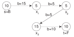
An example dataflow path with one source $s$ , one sink $t$ and three computational nodes $x_{1}$ , $x_{2}$ , $x_{3}$ is shown in Figure 3, with the node capacity and bandwidth requirements. $s$ and $t$ must be mapped on $B$ and $F$ , respectively. There can be many feasible mappings of this dataflow computation on the resource graph in Figure 1. One of them is –

\displaystyle M(s)

\displaystyle=

\displaystyle B

\displaystyle M(x_{1})

\displaystyle=

\displaystyle B

\displaystyle M(x_{2})

\displaystyle=

\displaystyle B

\displaystyle M(x_{3})

\displaystyle=

\displaystyle D

\displaystyle M(t)

\displaystyle=

\displaystyle F

\displaystyle M_{e}(s,x_{1})

\displaystyle=

\displaystyle(B,B)

\displaystyle M_{e}(x_{1},x_{2})

\displaystyle=

\displaystyle(B,B)

\displaystyle M_{e}(x_{2},x_{3})

\displaystyle=

\displaystyle(B,D)

\displaystyle M_{e}(x_{3},t)

\displaystyle=

\displaystyle(D,F)

which is also optimal in terms of total end-to-end latency of the resource nodes $M(s)$ and $M(t)$ .

2.3 . Computational Complexity of the Problem

We will now prove that BCPM problem is NP-complete. Since, BCPM is a special case of BCDM, NP-completeness of BCPM iplies that BCDM is an NP-hard problem. The NP-completeness proof of the BCPM problem is constructed by transformation of the Longest Path problem [2]. Definition of the decision version of the Longest Path problem is as follows -

Instance: A graph $G=(V,E)$ , a length function $l:E\rightarrow Z^{+}$ , specified vertices $s,t\in V$ and a positive integer $K$ . Question: Is there an $(s\leadsto t)$ simple path $P\subseteq G$ such that $\sum_{e\in P}{l(e)\geq K}$ ?

It is known that Longest Path problem is NP-complete, even for a special case, where $\forall_{e\in E}l(e)=1$ [2]. We will show that any instance of this special Longest Path problem can be polynomially transformed into an instance of BCPM.

2.3.1 . Longest Path $\propto$ BCPM

We construct an instance of BCPM as follows -

We take $G_{R}(V_{R},E_{R})=G(V,E)$ , $\forall_{v\in V_{R}}C_{av}(v)=1$ , $\forall_{e\in E_{R}}B_{av}(e)=1$ . Take a simple path $P_{J}=(V_{J},E_{J})$ such that $|V_{J}|=K$ , $\forall_{v\in V_{J}}C_{req}(v)=1$ and $\forall_{e\in E_{J}}B_{req}(e)=1$ .

Now, if there is a simple $(s\leadsto t)$ path of length $\geq K$ in G, then that path must have K hops, since $\forall_{e\in E}l(e)=1$ . Therefore, we can map $P_{J}$ along the corresponding path $P_{J}\prime$ in $G_{R}$ . If $|P_{J}\prime|>K$ , then we can map first $K-1$ nodes of $P_{J}$ on $P_{J}\prime$ and map the remaining edge $u_{K-1},u_{K}$ on the $v\leadsto t$ subpath of $P_{J}\prime$ , where $u_{K-1}$ is mapped on $v$ .

Given a mapping of the path $P_{J}$ on a path $P_{J}\prime\subseteq G_{R}$ that satisfies the capacity and bandwidth requirement constraints, $|P_{J}\prime|$ must be $>=K$ , because no two vertices of $P_{J}$ can be mapped on a single vertex of $|P_{J}\prime|$ given the abovementioned capacity constraints.

2.3.2 . BCPM $\in$ NP

Given an arbitrary mapping $M:V_{J}\rightarrow V_{R}$ one can polynomially verify -

•

Whether $C_{req}(v)\leq C_{av}(M(v))$ , for all $v\in V_{J}$ .
•

For each edge $(u,v)\in P_{J}$ , whether there is a $(M(u)\leadsto M(v))$ path in $G_{R}$ that satisfies the bandwidth constraint of $(u,v)$ (Similar to bandwidth constrained shortest path problem [10]).

This completes the proof that $BCPM\in NP$ - $C$ .

3 . Algorithm for path mapping problem

To solve the BCPM problem, we developed an algorithm using the the Bellman-Ford relaxation scheme. First, we present the centralized version of the algorithm, where the whole mapping is computed by a single node that has knowledge of the state of the whole network of nodes. Later, we explain the development of the distributed algorithm based on this centralized one.

This algorithm works by relaxing along each edge of the resource graph $N-1$ times, where $N=|V_{R}|$ , the number of nodes in the resource graph. For each node $u$ of the resource graph, a set of feasible mappings of different length prefixes of the dataflow-path on any resource path from the source node $s$ to the current node, is maintained. In each relaxation along an $(u,v)$ edge, any new feasible map on $(s\leadsto u)$ is extended in all possible ways, to complete the list of feasible maps of dataflow path-prefixes on the resource path $(s\leadsto u,v)$ and these new partial mappings are added to the set maintained for node $v$ . After $N-1$ iterations of relaxation of all edges, the map set maintained for terminal node $t$ contains all the feasible mappings of the dataflow-path on any $(s\leadsto t)$ resource path. The algorithm is presented in Algorithm 1, 2 and 3. A formal proof of the correctness of the algorithm is presented in the following sub-section. Lines $10$ - $12$ of the subroutine Relax is added to terminate the algorithm as soon as one feasible $(s\leadsto t)$ mapping is found. These lines should be omitted when optimal mapping is sought.

We have computed the computational complexity of the algorithm in Section 3.2. The complexity is bounded by polynomial of the size of the partial map set $S$ , although the set size is exponential. The problem being NP-hard, it is impossible to have a polynomially bounded optimal algorithm. However, heuristics may be applied to produce sub-optimal solutions within a tractable amount of complexity. A good way of designing such heuristics is to restrict the size of the map-set in some way. In Section 3.4 we have discussed several possible heuristics to solve the BCPM problem. Note that because the set of partial map is stored in each node, the memory complexity of the algorithm becomes exponential too. This can be avoided by omitting the storage of partial maps. Each partial map need to be stored for one iteration of relaxation only. If partial maps are deleted after relaxation, the set size never grows beyond $O(dp)$ , where, $d$ is the average indegree of a node in resource graph and $p=|P_{J}|$ is the number of nodes in the dataflow path.

1: for

x=0

|P_{J}|-1

2: if

\sum_{0\leq k\leq x}{C_{req}(k)}\leq C_{av}(s)

then

M(s,x)=\{m|m

maps initial

x

nodes of

P_{J}

s\}

4: else

5: break

6: end if

7: end for

8: for each vertex

v\in V_{R}-{s}

9: for

i=0

|P_{J}|

10:

M(v,i)=\phi

11: end for

12: end for

13: for

i=1

|V_{R}|-1

14: for each edge

e=(u,v)\in E_{R}

15: Relax(u,v)

16: end for

17: end for

Algorithm 1 Pathmap(

P_{J}

G_{R}

)

1: for

j=0

|P_{J}|

M_{tmp}(j)=null

3: end for

4: for

j=0

|P_{J}|-1

5: if

B_{req}(j,j+1)\leq B_{av}(u,v)

then

6: for each new mapping

m\in M(u,j)

in the last iteration do

7: if

v==t

then

m_{x}=

Extend(

m

, j,

|P_{J}|-j

, v)

M(v,|P_{J}|)=M(v,|P_{J}|)\cup m_{x}

10: if

M(v,|P_{J}|)\neq\phi

then

11: terminate the algorithm with

M(v,|P|)

as result

12: end if

13: else

14: for

x=0

|P_{J}|-j-1

15:

m_{x}=

Extend(m, j, x, v)

16: if

m_{x}\neq null

then

17:

M(v,j+x)=M(v,j+x)\cup m_{x}

18: else

19: break

20: end if

21: end for

22: end if

23: mark

m

as old

24: end for

25: end if

26: end for

Algorithm 2 subroutine Relax(u,v)

1: if

\sum_{1\leq k\leq x}{C_{req}(j+k)}\leq C_{av}(v)

then

2: extend

m

by putting computations

\{j+1,j+2,...,j+x\}

in node

v

3: let

m_{x}

be the extended mapping

4: else

m_{x}=null

6: end if

7: return

m_{x}

Algorithm 3 subroutine Extend(m, j, x, v)

3.1 . Correctness of BCPM algorithm

In this section we give a formal proof that when BCPM algorithm terminates, $M(t,|P_{J}|)$ always contains a feasible mapping of $P_{J}$ on $G_{R}$ if and only if such a feasible mapping exists.

Lemma 3.1.

If $M(u)=\bigcup_{\forall{j}}M(u,j)$ contains all feasible mappings of different length prefixes of $P_{J}$ on an path $(s\leadsto u)\in G_{R}$ , then after computing $\textbf{Relax}(u,v)$ , $M(v)$ includes all feasible mappings of different length prefixes of $P_{J}$ on the path $(s\leadsto u,v)\in G_{R}$ .

Proof.

By the construction of the $\textbf{Relax}(u,v)$ subroutine, each mapping $m\in M(u,j)$ , of a $j$ -length prefix of $P_{J}$ on a $(s\leadsto u)$ path, is extended over the $(u,v)$ edge exactly once. Any possible mapping of a $k$ -length prefix of $P_{J}$ on the $(s\leadsto u,v)$ path can be divided into 2 sub-mappings: a mapping of $j$ -length prefix $(j\leq k)$ of $P_{J}$ on $(s\leadsto u)$ path and a mapping of the following $k-j$ vertices of the $k$ -length prefix on $v$ . Since all feasible sub-mappings of the first kind is included in $M(u)$ and all the extensions of the second kind is considered in lines $8$ to $14$ and $15$ to $22$ of $\textbf{Relax}(u,v)$ , $M(v)$ contains all feasible mappings of any prefix of $P_{J}$ on $(s\leadsto u,v)$ paths. ∎

Lemma 3.2.

For any node $v\in V_{R}$ if there is a $s\leadsto v$ path $(v_{0}=s,v_{1},v_{2},...,v_{k}=v)$ of length $k$ , after $k$ th iteration of the outer for loop in line $7$ of the $PathMap$ algorithm, all feasible mappings of different length prefixes of $P_{J}$ on the $(v_{0}\leadsto v_{k})$ path has been recorded in $M(v)$ .

Proof.

We will prove by induction on $k$ . When $k=0$ , i.e. after the initialization phase, $M(v_{0},i)$ or $M(s,i),0\leq i\leq|P_{J}|$ contains the feasible $i$ -length prefix with first $i$ vertices of $P$ mapped on $s$ . So the basis is true.

Now let us assume that after $i-1$ iterations, $0<i\leq k$ , $M(v_{i-1})$ contains all feasible mappings of different lengths on the $(s\leadsto v_{i-1})$ portion of the $(s\leadsto v_{k})$ path. Since each edge in $E_{R}$ is considered once in each iteration, $Relax(v_{i-1},v_{i})$ must be called in the $i$ th iteration too. So, by Lemma 3.1, we can conclude that all feasible prefix mappings of $P_{J}$ on the $(s\leadsto v_{i})$ path is included in $M(v_{i})$ . ∎

Theorem 3.3.

After $|V_{R}|-1$ iterations of the outer loop in line $7$ algorithm $Pathmap$ , for each node $v\in V_{R}$ , $M(v)$ contains all feasible mappings of different length prefixes of $P_{J}$ on all possible $s\leadsto v$ paths.

Proof.

Since there is no simple path longer than $|V_{R}|-1$ , according to Lemma 3.2, all such paths will be covered by the $Relax$ procedure after $|V_{R}|-1$ iterations. ∎

The fact that after termination of $Pathmap$ , $M(t)$ contains all the feasible maps of $P_{J}$ on possible $(s\leadsto t)$ paths, follows directly from Theorem 3.3 with inclusion of lines $7$ to $12$ in the Relax procedure.

3.2 . Complexity of the algorithm

The problem size parameters are $|V_{R}|\equiv n$ , $|E_{R}|\equiv e$ and $|P_{J}|\equiv p$ . The outer loop of Pathmap is iterated $n-1$ times and each iteration considers each of the $e$ edges exactly once. So, the Relax procedure is called $ne$ times. In each relaxation over an edge $(u,v)$ , each of the $p$ prefix mappings from $M(u)$ is tried for relaxation into some of the $p$ mappings in $M(v)$ . A $j$ length prefix in $M(u,j)$ is tried for relaxation into $p-j$ of the $M(u,i),j\leq i\leq p$ , and each trial requires $(i-j)$ computations of constant complexity for the extension. Let $S$ be the maximum number of entries in the set of mappings $M(u,j),u\in V_{R},0\leq j\leq p$ . Note that only the new entries are relaxed in each iteration. However, the upper bound on the number of entries relaxed per $M(u,j)$ will be $S$ . So, the complexity of Relax(u,v) is –

	$\displaystyle S\sum_{j=0}^{p-1}{\left(\sum_{x=1}^{p-j-1}{x}+1\right)}$	$\displaystyle=$	$\displaystyle S\left(\frac{5}{12}p^{3}+\frac{1}{4}p^{2}+\frac{2}{3}p\right)$
		$\displaystyle=$	$\displaystyle O\left(\frac{5}{12}p^{3}{S}\right)$

So, the overall time complexity of the algorithm becomes $O(nep^{3}S)$ . We see that the sets $M(u,j)$ are creating the major load on both time and memory complexity of the algorithm. Therefore, restricting the growth of $S$ within polynomial limit would possibly result in a polynomial time approximation algorithm.

3.3 . Distributed version of the algorithm

The centralized algorithm can be easily extended to a distributed version, where each node $u$ in the resource network $G_{R}$ will maintain the data structure $M(u)$ of partially computed mappings. Also, node $u$ will be responsible for computing the relaxation to each of its neighbors $v$ in $G_{R}$ . The extended mappings are then transmitted to $v$ . The relaxation procedure is invoked by a node $u$ when any new mapping arrives from any of its incoming neighbors. The algorithm is formally laid out in Algorithm 4. Upon arrival of a map message $m$ , a node $u$ process the message using the algorithm ProcessMap(u, m). It follows from the correctness of the centralized algorithm that the distributed mapping completes after at most $N-1$ ProcessMap invocation by each node in the graph. The distributed mapping algorithm can be terminated by force as soon as the terminal nodes receives a complete mapping. Otherwise, the algorithm terminates after all the outstanding ProcessMap have been completed. Since cycles are avoided during extension, an initial mapping may be extended at most $N-1$ times. Thus there will be a finite number of ProcessMap invocation and the algorithm will terminate after a finite amount of time.

1: Map message contains the mapping of computation nodes

0

1

2

, … ,

j

on resource nodes. The first message to a node contains the requirement definition of the computation too

j=|m|

3: if

u==t

then

m_{x}=

Extend(

m

, j,

|P_{J}|-j

, u)

5: if

m_{x}\neq null

then

6: terminate the algorithm with

m_{x}

as result

7: end if

8: else

9: for

x=0

|P_{J}|-j-1

10:

m_{x}=

Extend(m, j, x, u)

11: if

m_{x}\neq null

then

12: for each neighbor

v

u

that is not already in

m

13: if

B_{req}(j+x,j+x+1)\leq B_{av}(u,v)

then

14: extend

m_{x}

m_{x}x

by appending a map of

0

computations on node

v

15: send

m_{x}x

v

16: end if

17: end for

18: end if

19: end for

20: end if

Algorithm 4 ProcessMap(u, m)

3.4 . Heuristic Approaches to Reduce Complexity

Computational complexity of both the centralized and the distributed path mapping algorithm grows exponentially with the problem size. Therefore, for practical deployment, we need some heuristic that produces good approximation to the optimal result. Here we discuss three possible heuristics that modifies the original algorithm to reduce computational, messaging and memory complexity.

3.4.1 . LeastCostMap

One major source of growth in complexity of the algorithm is the exponential growth of the set of partial maps maintained for each node. In the LeastCostMap heuristic, only one partial map of each prefix-length is maintained for each node. If a new map is generated, the cost of the new map in terms of the additive quality metric is compared with that of the already stored one, and the map with higher cost is discarded. This policy reduces the complexity to $O(p^{3})$ .

Similar policy can be applied to the distributed version of the algorithm. However, in the distributed case, a map message is expanded to its neighbors as soon as the message is received. So, if a higher cost map message is arrived before a lower cost one, the processing of the higher cost message cannot be pruned. However, in most cases, higher cost messages arrive later, so they are pruned.

We have implemented both the centralized and distributed version of the original algorithm and also the LeastCostMap heuristic. The algorithms are then applied on random topologies generated by the BRITE Internet topology generator [7] and randomly generated dataflow paths. Due to the huge computational complexity of the exact algorithm, it was not possible to run it for networks larger than $50$ nodes. For these networks, the heuristic is able to find the optimal solution in $99\%$ of the cases, with $100$ to $1000$ fold reduction in the size of the set of partial maps. For similar topologies, the distributed version of the heuristic produced optimal result in more than $99\%$ cases and total number of message exchange was reduced approximately $100$ fold.

3.4.2 . AnnealedLeastCostMap

One way of trading off between optimality and complexity of the LeastCostMap heuristic is to apply a simulated annealing approach to decide whether to discard a higher cost partial map from the set in presence of a lower cost map. As the temperature of the process anneals, i.e. at the later iterations, the probability of keeping a non-minimal partial solution will decrease. Definitely this approach increases the computation and message complexity. However, this allows some of the non-minimal partial solutions to grow and possibly lead to a better complete solution.

3.4.3 . RandomNeighbor

Another way of restricting the message complexity is to extend any partial map to a randomly chosen subset of $k$ neighbors instead of expanding to all of them. Higher values of $k$ increases the chance of getting the optimal solution. The RandomNeighbor heuristic with $k=1$ did not produce results as good as LeastCostMap, although number of messages were reduced dramatically. Further investigation need to be done to determine a suitable value of $k$ .

4 . Conclusion

In this paper we have developed and explained a decentralized algorithm to compute the optimal mapping of computational capacity and network bandwidth requirement of a data-flow computation. Many high-throughput scientific research platforms need to support applications that resemble data-flow computation. The discussion presented in this paper provides in-depth understanding of the resource allocation problem for such computations and demonstrates the way to develop cost-effective solutions. At this point, the algorithm supports computations with path-topology only. Several interesting applications such as complex continual queries on data stream originating from multiple sites, resemble a tree topology. A possible extension of this work is to modify the algorithm such that mapping of flow-computations with different topologies can be obtained.

References

[1] S. Chen and K. Nahrstedt. On finding multi-constrained paths. In Proc. IEEE ICC, pages 874–879, Jun. 1998.
[2] M. R. Garey and D. S. Johnson. Computers and Intractability: A Guide to the Theory of NP-Completeness. W H Freeman Co., NY, USA, 1979.
[3] X. Gu and K. Nahrstedt. Distributed multimedia service composition with statistical QoS assurances. IEEE Trans. Multimedia, 8(1):141–151, 2006.
[4] V. Kumar, B. F. Cooper, Z. Cai, G. Eisenhauer, and K. Schwan. Resource aware distributed stream management using dynamic overlays. In Proc. 25th IEEE ICDCS, pages 783–792, Jun. 2005.
[5] J. Liang and K. Nahrstedt. Service composition for generic service graphs. Multimedia Systems, 11(6):568–581, 2006.
[6] B. Ludscher, I. Altintas, C. Berkley, D. Higgins, E. Jaeger, M. Jones, E. A. Lee, J. Tao, and Y. Zhao. Scientific workflow management and the kepler system. Concurrency and Computations: Practice and Experience, 18(10):1039–1065, 2006.
[7] A. Medina, A. Lakhina, I. Matta, and J. Byers. BRITE: an approach to universal topology generation. In Proc. 9th Intl. Symp. on Modeling, Analysis and Simulation of Computer and Telecommunication Systems, pages 346–353, Aug. 2001.
[8] M. Song and S. Sahni. Approximation algorithms for multiconstrained quality-of-service routing. IEEE Trans. Computers, 55(5):603–617, 2006.
[9] M. Wang, B. Li, and Z. Li. sFlow: Towards resource-efficient and agile service federation in service overlay networks. In Proc. 24th IEEE ICDCS, pages 628–635, Mar. 2004.
[10] Z. Wang and J. Crowcroft. Quality of service routing for supporting multimedia applications. IEEE J. Selected Areas in Communications, 14(7):1228–1234, 1996.

Towards a Decentralized Algorithm for Mapping Network and Computational Resources for Distributed Data-Flow Computations

Abstract

1 . Introduction

2 . Problem Formulation

2.1 . Capacity Constrained Graph Mapping Problem

2.2 . Constrained Path Mapping Problem

2.3 . Computational Complexity of the Problem

2.3.1 . Longest Path ∝\propto BCPM

2.3.2 . BCPM ∈\in NP

3 . Algorithm for path mapping problem

3.1 . Correctness of BCPM algorithm

Lemma 3.1.

Proof.

Lemma 3.2.

Proof.

Theorem 3.3.

Proof.

3.2 . Complexity of the algorithm

3.3 . Distributed version of the algorithm

3.4 . Heuristic Approaches to Reduce Complexity

3.4.1 . LeastCostMap

3.4.2 . AnnealedLeastCostMap

3.4.3 . RandomNeighbor

4 . Conclusion

References

2.3.1 . Longest Path $\propto$ BCPM

2.3.2 . BCPM $\in$ NP