Stability of marginally outer trapped surfaces and symmetries
Abstract
We study properties of stable, strictly stable and locally outermost marginally outer trapped surfaces in spacelike hypersurfaces of spacetimes possessing certain symmetries such as isometries, homotheties and conformal Killings. We first obtain results for general diffeomorphisms in terms of the so-called metric deformation tensor and then particularize to different types of symmetries. In particular, we find restrictions at the surfaces on the vector field generating the symmetry. Some consequences are discussed. As an application we present a result on non-existence of stable marginally outer trapped surfaces in slices of FLRW.
1 Introduction
Trapped surfaces, and their various relatives, are fundamental objects in Classical General Relativity. Being quasilocal versions of black holes, their study is essential in order to understand how black holes evolve when no global assumptions are made in the spacetime, for instance in order to address the cosmic censorship conjecture (see e.g. [1]). They are also widely used in numerical relativity.
It is often the case that trapped surfaces (which will always be taken to be closed in this paper) have to be studied in spacetimes possessing some kind of symmetry. This is the case, for instance, when configurations of equilibrium are considered, or in spherically symmetric or axially symmetric configurations. However, not only isometries are important in this respect. For instance, critical collapse is a universal feature of many matter models and the critical solution, which separates those configurations that disperse from those that form black holes, is known to admit either a continuous or a discrete self-similarity. This makes it interesting to study trapped surfaces in spacetimes with homothetic Killing vectors. Many relevant spacetimes admit other types of symmetries, like for instance conformal symmetries, e.g. in FLRW cosmologies. Therefore, it becomes interesting to study the relationship between trapped surfaces and special types of vectors. A recent example of this interplay has been given in [2], [3], where the localization of the boundary of the set containing trapped surfaces, which is a natural candidate for the ”surface of an evolving black hole”, was analyzed in the Vaidya spacetime, which is one of the simplest dynamical situations. In this analysis the presence of a so-called Kerr-Schild symmetry (see e.g. [4]) turned out to be fundamental.
In the important case of isometries, general results on the relationship between trapped surfaces and Killing vectors were discussed in [5]. The first variation of area was used to obtain several restrictions on the existence of trapped and marginally trapped surfaces in spacetime regions possessing a causal Killing vector. More specifically, if the Killing vector is timelike in some region, then no trapped surface can exist there, and marginally trapped surfaces can only exist if their mean curvature vanishes identically. By obtaining a general identity for the first variation of area in terms of the deformation tensor of an arbitrary vector (see below for the definition) similar restrictions were obtained for spacetimes admitting other types of symmetries, like conformal Killing vectors or Kerr-Schild vectors. The same idea was also applied in [6] to obtain analogous results in spacetimes with vanishing curvature invariants.
The interplay between isometries and dynamical horizons (which are spacelike hypersurfaces foliated by marginally trapped surfaces) was considered in [7] where it was proven that regular dynamical horizons cannot exist in spacetime regions containing a nowhere vanishing causal Killing vector, provided the spacetime satisfies the null energy condition (NEC).
One of the most relevant variants of trapped surfaces are the so-called marginally outer trapped surfaces (MOTS), where only the expansion along the outer null vector becomes restricted. The relation between stable MOTS and isometries was considered in [8], where it was shown that, given a strictly stable MOTS in a hypersurface (not necessarily spacelike), any Killing vector tangent to on must in fact be tangent to .
MOTS in stationary or static spacetimes play a particularly relevant role. Indeed, MOTS are believed to be good replacements of black holes, so a natural question arises of whether or not some version of the black hole uniqueness theorems also holds for asymptotically flat equilibrium configurations containing MOTS. This was answered in the affirmative by P. Miao [9] in the static, vacuum case when the MOTS lies in a time symmetric slice (hence, it is a minimal surface) and bounds a domain. A general study of MOTS in stationary and static spacetimes with arbitrary matter contents satisfying NEC was performed in [10]. In the stationary case, it was proven that, on an arbitrary spacelike hypersurface , no bounding MOTS lying in the exterior region where the Killing field is causal can penetrate into the timelike region. This result was strengthened for static Killing vectors: no bounding MOTSs can penetrate in the exterior region where the static Killing vector is timelike. The underlying idea of [10] was to take the outermost MOTS and construct another weakly outer trapped surface which lies outside of , at least partially, thus contradicting the outermost property of . The new surface was constructed by first moving to the past of along the integral lines of the Killing vector some amount and then back to along the outgoing future null geodesics. The intersection of this hypersurface with defines a new surface , which is automatically located partially outside of if the Killing is timelike somewhere on . Furthermore, the shift of along the isometry obviously gives a new MOTS, while the outer expansion cannot increase in the translation along the null geodesics, due to the Raychaudhuri equation. Hence the whole procedure gives a weakly outer trapped surface, and therefore a contradiction.
In the present work, we will study the interplay between stable and outermost properties of marginally outer trapped surfaces in spacetimes possessing special types of vector fields, including isometries, homotheties, conformal Killing vectors and many others. In fact, we will find several results involving completely general vector fields . The initial idea is to analyze in detail the geometric construction of outlined above in order to find restrictions on on an outermost MOTS in a given spacelike hypersurface , or alternatively, forbid the existence of a MOTS in certain regions where fails to satisfy those restrictions. The collection of defines a variation of within . The corresponding first order variation of the outer null expansion is an elliptic operator acting on a function which is precisely the function which, at first order, determines whether lies outside of or not. This observation, as such, is of little use until the operator can be directly linked to the vector field , and more specifically, to its deformation tensor. The standard expression for the stability operator (see e.g. [8]) has a priori nothing to do with the properties of the vector field . The first task is, therefore, to obtain an alternative (and completely general) expression for in terms of the deformation tensor of . We devote Section 3 to do this. The result, given in Proposition 1 below, is thoroughly used in this paper and also has independent interest.
With this expression at hand, we can already analyze under which conditions the procedure above gives restrictions on . In Sect.4 we concentrate on the case where has a sign everywhere on . It turns out that the results obtained by the geometric construction above can, in most cases, be sharpened considerably by using the maximum principle of elliptic operators. This also allows one to extend the validity of the results from the outermost case to the case of stable and strictly stable MOTS. The main result of Sect.4 is given in Theorem 1, which holds for any vector field . This result is then particularized to conformal Killing vectors (including homotheties and Killing vectors). Under the additional restriction that the homothety or the Killing vector is everywhere causal and future (or past) directed, strong restrictions on the geometry of the MOTS are derived (Corollary 3). As a consequence, we prove that in a plane wave spacetime any stable MOTS must be orthogonal to the direction of propagation of the wave. Marginally trapped surfaces are also discussed in this section.
As an explicit application of the results on conformal Killing vectors, we show, in subsection 4.1, that MOTS which are stable with respect to any spacelike direction cannot exist in FLRW cosmological models provided the density and pressure satisfy the inequalities , and . This includes, for instance, all classic models of matter and radiation dominant eras and also those models with accelerated expansion which satisfy NEC. Subsection 4.2 deals with one case where, in contrast with the standard situation, the geometric construction does in fact give sharper results than the elliptic theory.
In the case when is not assumed to have a definite sign, the maximum principle looses its power. However, the geometric construction can still be used despite the fact that the surfaces are necessarily not weakly outer trapped (for small enough). This is studied in Section 5, where we exploit a smoothing argument by Kriele and Hayward [11] which allows one to construct, out of two intersecting surfaces, a smooth surface which lies outside of them and has smaller outer expansion than the original ones. This gives a result (Theorem 5) which holds for general vector fields on any locally outermost MOTS. As in the previous section, we then particularize to conformal Killing vectors, and then to causal Killing vectors and homotheties which, in this case, are allowed to change their time orientation on .
We start with the basic definitions and results needed for this work.
2 Basics
Consider a spacetime and a vector field defined on it. The Lie derivative describes how the metric is deformed along the local group of diffeomorphisms generated by . We thus define the metric deformation tensor associated to , or simply deformation tensor, as
| (1) |
Special forms of define special types of vectors. In particular, ( a scalar function) defines a conformal Killing vector, ( a constant) corresponds to a homothety and defines a Killing vector.
As described in the Introduction, we want to relate the deformation tensor of special vectors to the stability and outermost properties of MOTS. We will denote by a smooth, closed (i.e. compact and without boundary) and orientable surface embedded in a spacelike hypersurface . The future directed unit vector normal to will be called and the unit vector orthogonal to along is called . The null vectors and are a null basis of the normal bundle of , and satisfy (scalar product with the spacetime metric is denoted by ). These vectors are univocally defined once a choice of orientation for is made.
The first fundamental form of is a Riemannian metric which we denote by . At any point , the tangent space decomposes as the direct sum of the tangent and normal vector spaces to . This splits any vector as . The second fundamental form vector of is defined as where is a basis of . Finally, the mean curvature vector is the trace of the second fundamental form, . Being a normal vector, it can be expanded in the null basis as
where the coefficients define the null expansions , of along and , respectively. Similarly, the expansion along any normal direction is defined as and the second fundamental form along is .
A useful classification of surfaces arises depending on the causal character of or on the sign of one of the expansions. Assume that one preferred orientation of can be selected geometrically. We call this the outer direction. The corresponding null vector is the outer null direction. If, furthermore, separates in two regions, we will call “exterior” the portion to which the outer direction points.
The types of surfaces that will play a role in this paper are (see [12] for an exhaustive classification): is marginally future (past) trapped if points along one of the null normals, or , and is future (past) pointing at each point (in our convention, the vanishing vector is both future and past null), is weakly outer trapped if and is marginally outer trapped surface (MOTS) provided .
This work basically deals with properties of (strictly) stable and locally outermost MOTSs, defined as follows [13]. is stable11 1 Strictly speaking we should say stable in . However, we will only deal with one hypersurface at a time, and no confusion should arise. if there exists a function , on such that the variation of along , denoted by , is non-negative. is strictly stable if, moreover, somewhere on . As described in [13], the variation gives a linear second order elliptic operator acting on , which we will denote by . The explicit form of this operator appears in equation (1) of [13]. It is also well-known [13, 8] that stability can be rephrased in terms of the sign of principal eigenvalue of (defined to have the smallest real part, and which is always real): is stable if and strictly stable if .
A MOTS is locally outermost if there exists a two-sided neighbourhood of on whose exterior part does not contain any weakly outer trapped surface. We will denote by the interior part of this two-sided neighbourhood.
The relationship between these types of surfaces is the following [13]: (i) a strictly stable MOTS is necessarily locally outermost, (ii) a locally outermost MOTS is necessarily stable, and (iii) none of the converses is true in general.
The results obtained in Sect.4 below use the following version of the maximum principle for second order linear elliptic operators [8] (recall that the eigenspace corresponding to the principal eigenvalue is one-dimensional and no function in this space can change sign).
Lemma 1
Consider a second order linear elliptic operator on a compact manifold with principal eigenvalue and principal eigenfunction and let be a smooth function satisfying ().
- 1.
If , then and for some constant
- 2.
If and , then () all over .
- 3.
If and , then .
As mentioned in the Introduction, the idea we want to apply in order to obtain restrictions on a given vector field on a MOTS consists in moving first along the integral lines of a parametric amount . This gives a new surface . Take the null normal on this surface which coincides with the continuous deformation of and consider the null hypersurface generated by null geodesics with tangent vector . This hypersurface is smooth close enough to . Being null, its intersection with the spacelike hypersurface is transversal and hence defines a smooth surface (for sufficiently small). By this construction, a point on describes a curve in . The tangent vector of this curve on , denoted by , will define the variation vector generating the deformation of . Figure 1 gives a graphic representation of this construction.
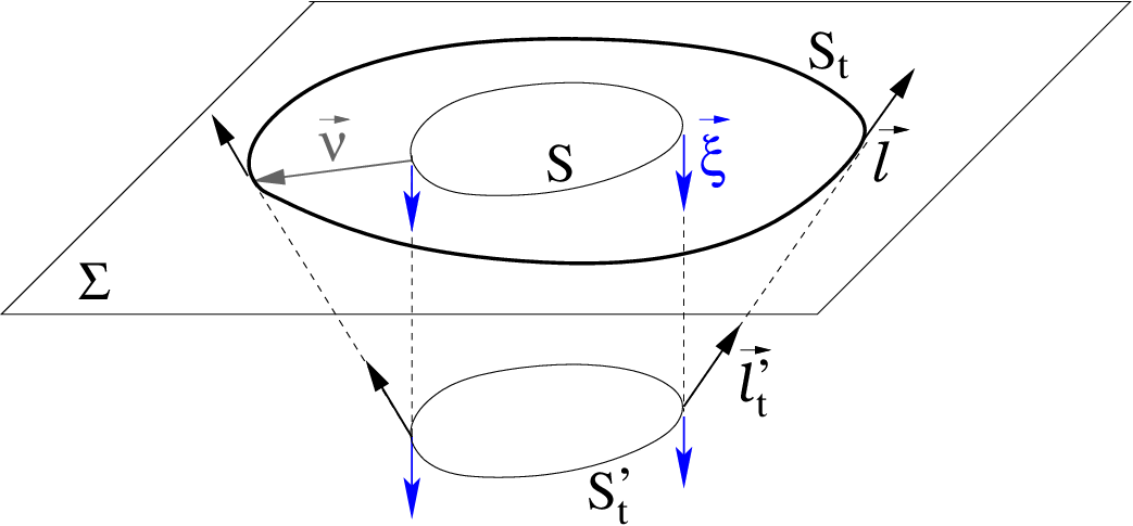
As usual, we decompose the vector into normal and tangential components with respect to , as . On we will further decompose in terms of a tangential component , and a normal component , i.e. , where is the value of on the surface. Since defines the variation of to first order, we only need to evaluate the vector to zero order in , which obviously coincides with . It follows that is a linear combination (with functions) of and . The amount we need to move in order to go back to can be determined by imposing to be tangent to . This gives , where
| (2) |
Since the tangential part of does not affect the variation of along for a MOTS, it follows that . Then, a direct application of Lemma 1 for a MOTS with stability operator leads to the following result.
Lemma 2
Let be a stable MOTS on a spacelike hypersurface . If () and not identically zero, then ().
Furthermore, if is strictly stable and () then () and it vanishes at one point only if it vanishes everywhere on .
This result will be used in Sect.4 to obtain restrictions on the vector field on stable and strictly stable MOTS. The idea is to use the deformation tensor to obtain an independent expression for . Consider the simplest example of a Killing vector . Since the null expansion does not change under an isometry, it follows that the surface is also a MOTS. Moving back to along the null hypersurface gives a contribution to which, from the Raychaudhuri equation, is easily computed to be , where we have introduced the shorthand notation
| (3) |
with being the Einstein tensor of and the square of the second fundamental form along , which coincides with the square of the shear along in the case of MOTS. Note that is non-negative provided the null energy condition (NEC) holds. i.e. for any null vector . It is clear that under NEC Lemma 2 implies restrictions on any Killing vector on a stable MOTS.
However, obtaining the result directly from the explicit form of the elliptic operator is not trivial because the condition of being a Killing vector does not give obvious restrictions on the coefficients of this operator. In the case of Killing vectors, the point of view of moving along and then back to gives a simple method of calculating . For more general vectors, however, the motion along will give a non-zero contribution to which needs to be computed (for Killing vectors this term was known to be zero via a symmetry argument, not from a direct computation). In order to do this, it becomes necessary to have an alternative, and completely general, expression for directly in terms of the deformation tensor of .
3 Variation of the expansion and the metric deformation tensor
The aim of this section is to derive an identity for in terms of . This result will be important later on in this paper, and may also be of independent interest. We derive this expression in full generality, i.e. without assuming to be a MOTS and for the expansion along any normal vector of , not necessarily a null normal.
To do this calculation, we need to take derivatives of tensorial objects defined on each one of . For a given point , these tensors live on different spaces, namely the tangent spaces of , where is the local diffeomorphism generated by . In order to define the variation, we need to pull-back all tensors to the point before doing the derivative. We will denote the resulting derivative by . This is, in fact, an abuse of notation because we are not taking Lie derivatives of tensor fields on the manifold (they are tensorial objects on each but these surfaces may perfectly well intersect each other). Nevertheless, it is a useful notation because when acting on spacetime tensor fields (e.g. the metric ) the operation involved is really the standard Lie derivative along . This will simplify the calculation considerably.
Notice in particular that the definition of depends on the choice of on each of the surfaces . Thus will necessarily include a term of the form which is not uniquely defined (unless can be uniquely defined on each which is usually not the case). Nevertheless, for the case of MOTS and when this a priori ambiguous term becomes determined, as we will see. The general expression for is given in the following proposition.
Proposition 1
Let be a surface on a spacetime , a vector field defined on with deformation tensor and a vector field normal to . Then, the variation along of the expansion on reads
| (4) |
where .
Proof. Since , the variation we need to calculate involves three terms
| (5) |
In order to do the calculation, we will choose as the basis of tangent vectors at . This entails no loss of generality and implies , which makes the calculation simpler. Our aim is to express each term of (5) in terms of . For the first term, we need to calculate . We start with , which immediately implies , so that the first term in (5) becomes
| (6) |
where capital Latin indices are lowered and raised with and its inverse.
The second term is more complicated. It is useful to introduce the projector to the normal space of , . From the previous considerations, it follows that , which implies
| (7) |
where we have used the fact that is orthogonal to , so its contraction with vanishes.
Therefore we only need to evaluate . It is well-known (and in any case easily verifiable) that for an arbitrary vector field , the commutation of the covariant derivative and the Lie derivative introduces a term involving the Riemann tensor of , as follows
This expression is still true for the variational derivative we are calculating. Thus, we have
| (8) |
It only remains to express the quantity in terms of . To that aim, we take a derivative of equation (1) and use the Ricci identity to get
Now, write the three equations obtained from this one by cyclic permutation of the three indices. Adding two of them and subtracting the third one we find, after using the first Bianchi identity,
Substituting (8) and this expression into (7) yields
| (9) |
We can now particularize to the outer null expansion in a MOTS.
Corollary 1
If is a MOTS then
| (10) |
Proof. The normal vector defined on each of the surfaces is null. Therefore, using ,
| (11) |
Since, on a MOTS , it follows , and the corollary follows from (4).
Remark. From the proof, it is clear that we have only used at . Therefore formula (10) holds in general for arbitrary surfaces at any point where .
4 Results provided has a sign on
The most favorable case to obtain restrictions on the generator on a given MOTS is when the surfaces constructed by the procedure above are weakly outer trapped. This is guaranteed for small enough when is strictly negative everywhere, because then this first order term becomes dominant. Suppose that in addition of being a MOTS is also outermost, in the intuitive sense that no other weakly outer trapped surface can penetrate in its exterior (we will give a more precise definition below). Since the direction to which a point moves is determined to first order by the vector , it is clear that at any point implies that for small enough , lies partially in the exterior of . Combining these facts, it follows that everywhere and somewhere is impossible for an outermost MOTS. This argument is intuitively very clear. However, this geometric method does not provide the most powerful way of finding this type of restrictions. Indeed, when the first order term vanishes at some points, then higher order coefficients come necessarily into play, which makes the geometric argument involved. It is remarkable that using the elliptic results described in Sect. 2, most of these situations can be treated in a satisfactory way. Furthermore, since the elliptic methods only use infinitesimal information, there is no need to restrict oneself to outermost MOTS, and the more general case of stable or strictly stable surfaces can be considered. In this section we will give several results along these lines. The general idea is to combine Lemma 2 with the general calculation for the variation of obtained in the previous section to get restrictions on special types of generators on a stable or strictly stable MOTS.
Our first result is fully general in the sense that it is valid for any generator .
Theorem 1
Let be a stable MOTS on a spacelike hypersurface and a vector field on with deformation tensor . With the notation above, define
| (12) |
and assume everywhere on .
- (i)
If somewhere, then everywhere.
- (ii)
If is strictly stable, then everywhere and vanishes at one point only if it vanishes everywhere.
Remark. The theorem also holds if all the inequalities are reversed. This follows directly by replacing .
Proof. Consider the first variation of defined by the vector . From the definition of stability operator [8], we have . On the other hand, linearity of this variation gives . Using now the Raychaudhuri equation (see (3)) and the identity (10) gives . Since , the result follows directly from Lemma 2.
This theorem gives information about the relative position between the generator and the outer null normal and has, in principle, many potential consequences. Specific applications require considering spacetimes having special vector fields for which sufficient information about its deformation tensor is available. Once such a vector is known to exist, the result above can be used either to restrict the form of in stable or strictly stable MOTS or, alternatively, to restrict the regions of the spacetime where such MOTS are allowed to be present.
Since conformal vector fields (and homotheties and isometries as particular cases) have very special deformation tensors, the theorem above gives interesting information for spacetimes admitting such symmetries.
Corollary 2
Let be a stable MOTS in a hypersurface of a spacetime which admits a conformal Killing vector , (including homotheties , and isometries ).
- (i)
If and not identically zero, then .
- (ii)
If is strictly stable and then and vanishes at one point only if it vanishes everywhere
Remark. As before, the theorem is still true if all inequalities are reversed.
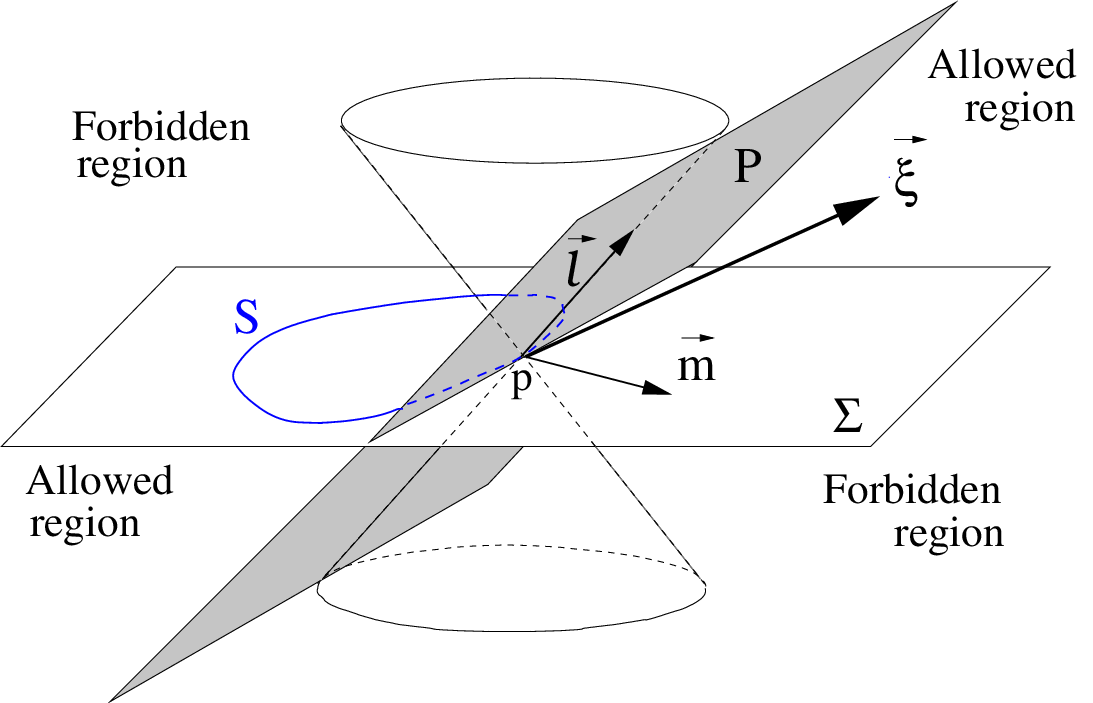
Remark. In the case of homotheties and Killing vectors, the condition of the theorem demands that . Under NEC, this holds provided , i.e. when points below everywhere on (where the term “below” includes also the tangential directions). For strictly stable , the conclusion of the theorem is that the homothety or the Killing vector must lie above the null hyperplane defined by the tangent space of and the outer null normal at each point . If the MOTS is only assumed to be stable, then the theorem requires the extra condition that points strictly below at some point with . However, the conclusion is also stronger and forces to lie strictly above the null hyperplane everywhere. By changing the orientation of , it is clear that similar restrictions arise when is assumed to point above . Figure 2 summarizes the allowed and forbidden regions for in this case.
Proof. We only need to show that for conformal Killing vectors. This follows at once from (12) and after using orthogonality of and . Notice in particular that is the same for isometries and for homotheties.
This corollary has an interesting consequence in spacetime regions where there exists a Killing vector or a homothety which is causal everywhere.
Corollary 3
Let a spacetime satisfying NEC admit a causal Killing vector or homothety which is future (past) directed everywhere on a stable MOTS . Then,
- (i)
The second fundamental form along and vanish identically on every point where .
- (ii)
If is strictly stable, then everywhere.
Remark. If we assume that there exists an open neighbourhood of in where the Killing vector or homothety is causal and future (past) directed everywhere then the conclusion (i) can be strengthened to say that and vanish identically on . The reason is that such a cannot vanish anywhere in this neighbourhood (and consequently neither on ). For Killing vectors this result is proven in Lemma 3.2 in [14] and a simple generalization shows that the same holds for homothetic Killing vectors.
Proof. We can assume, after reversing the sign of if necessary, that is past directed, i.e. .
Under NEC, is the sum of two non-negative terms, so in order to prove (i) we only need to show that on points where , i.e. at points where . Assume, on the contrary, that and happen simultaneously at a point . It follows that everywhere and non-zero at . Thus, we can apply statement (i) of Corollary 2 to conclude everywhere. Hence and not identically zero on . Recalling the decomposition , the square norm of this vector is
| (13) |
This is the sum of non-negative terms, the first one not identically zero. This contradicts the condition of being causal.
To prove the second statement, we notice that point (ii) in Corollary 2 implies , and hence . The only possibility how (13) can be negative or zero, is , i.e. .
This corollary extends Theorem 2 in [5] to the case of stable MOTS and implies, for instance, that any strictly stable MOTS in a plane wave spacetime (which by definition admits a null and nowhere zero Killing vector field ) must be aligned with the direction of propagation of the wave (in the sense that must be one of the null normals to the surface). It also implies that any spacetime admitting a causal and future directed Killing vector (or homothety) whose energy-momentum tensor does not admit a null eigenvector (e.g. a perfect fluid) cannot contain any stable MOTS.
The results above hold for stable or strictly stable MOTS. Among such surfaces, marginally trapped surfaces are of special interest. Our next result restricts (and in some cases forbids) the existence of such surfaces in spacetimes admitting Killing vectors, homotheties or conformal Killings.
Theorem 2
Let be a stable MOTS in a spacelike hypersurface of a spacetime which satisfies NEC and admits a conformal Killing vector with conformal factor (including homotheties with and Killing vectors). Suppose furthermore that either (i) or (ii) is strictly stable and . Then the following holds.
- (a)
If then cannot be a marginally future trapped surface, unless . The latter case is excluded if .
- (b)
If then cannot be a marginally past trapped surface, unless . The latter case is excluded if .
Remark. The statement obtained from this one by reversing all the inequalities is also true. This is a direct consequence of the freedom in changing .
Proof. We will only prove case (a). The argument for case (b) is similar. The idea is taken from [5] and consists of performing a variation of along the conformal Killing vector and evaluate the change of area in order to get a contradiction if is marginally future trapped. The difference is that here do not make any a priori assumption on the causal character for . Corollary 2 provides us with sufficient information for the argument to go through.
As before, let be the collection of surfaces obtained by displacing with the local diffeomorphism generated by a parametric amount . We denote by their corresponding areas. The first variation of area (see e.g. [5]) gives
| (14) |
where is the volume form of and we have used . Now, since , and furthermore either hypothesis (i) or (ii) holds, Corollary 2 implies that .
On the other hand, being a conformal Killing vector, the induced metric on is related to the metric on by conformal rescaling. A simple calculation gives (see e.g. [5])
| (15) |
This quantity is non-negative due to and not identically zero if somewhere. Combining (14) and (15) we conclude that if (i.e. is marginally future trapped) then necessarily vanishes identically (and so does ). Furthermore, if is non-zero somewhere, then must necessarily be positive somewhere, and cannot be future marginally trapped.
4.1 An application: No stable MOTSs in FLRW
In this subsection we apply Corollary 2 to show that a large subclass of Friedmann-Lemaître-Robertson-Walker (FLRW) spacetimes do not admit stable MOTS on any spacelike hypersurface. Obtaining the corresponding results for round spheres only requires a straightforward calculation, and is therefore simple. The power of the method is that it provides a general result involving no assumption on the geometry of the MOTS or on the spacelike hypersurface where it is embedded. The only requirement is that the scale factor and its time derivative satisfy certain inequalities. This includes, for instance all FLRW cosmologies satisfying NEC and with accelerated expansion, as we shall see in Corollary 4 below.
Recall that the FLRW metric is
where is the scale factor and for respectively. The Einstein tensor of this metric is of perfect fluid type (see e.g. [15]) and reads
| (16) |
where dot stands for derivative with respect to .
Theorem 3
There exists no stable MOTS in any spacelike hypersurface of a FLRW spacetime satisfying
| (17) |
Remark. In terms of the energy-momentum contents of the spacetime, these three conditions read, respectively, , and . As an example, in the absence of a cosmological constant they are satisfied as soon as energy conditions are imposed and the pressure is not too large (e.g. for the matter and radiation dominated eras). The class of FLRW satisfying (17) is clearly very large. We also remark that Theorem 3 agrees with the fact [16] that the causal character of the hypersurface which separates the trapped from the non-trapped spheres in FLRW spacetimes depends precisely on the quatity .
Proof. The FLRW spacetime admits a conformal Killing vector with conformal factor . Since this vector is timelike and future directed, it follows that for any spacelike surface embedded in a spacelike hypersurface . If we can show that , and non-identically zero for any , then point (i) in Corollary (2) implies that cannot be a stable MOTS, thus proving the result. The proof therefore relies on finding conditions on the scale factor which imply the validity of this inequality on any . First of all, we notice that the second fundamental form can be made as small as desired on a suitably chosen . Thus, the inequality that needs to be satisfied is
| (18) |
and positive somewhere. In order to evaluate this expression recall that . Let us write , where is unit and let be the hyperbolic angle of in the basis , i.e. . It follows immediately that and . Furthermore, multiplying by the normal vector to the surface we find , where is the angle between and . With this notation, let us calculate the null vector . Writing , with orthogonal to , it follows from the condition of being null. On the other hand we have the decomposition . Multiplying by we immediately get , and since only depends on
| (19) |
The following expression for follows directly from and (16),
| (20) |
Inserting (19) and (20) into (18) and dividing by (which is positive) we find the equivalent condition
| (21) |
and non-zero somewhere. The dependence on only arises through the function . Rewriting this as it is immediate to show that takes all values in . Hence
In order to satisfy (21) on all this range, it is necessary and sufficient that the two inequalities in (17) are satisfied
The following Corollary gives a particularly interesting case where all the conditions of Theorem 3 are satisfied.
Corollary 4
Consider a FLRW spacetime satisfying NEC. If , then there exists no stable MOTS in any spacelike hypersurface of
Proof. The null energy condition gives . This implies the first two inequalities in (17) if . The remanining condition is also obviously satisfied provided .
4.2 A consequence of the geometric construction of
We have emphasized at the beginning of this section that the restrictions obtained directly by the geometric procedure of moving along and then back to are intuitively clear but typically weaker than those obtained by using elliptic theory results. There are some cases, however, where the reverse actually holds, and the geometric construction provides stronger results. We will present one of these cases in this subsection.
Corollary 2 gives restrictions on for Killing vectors and homotheties in spacetimes satisfying NEC, provided is future or past directed everywhere. However, when vanishes identically, the result only gives useful information in the strictly stable case. The reason is that implies and, for marginally stable surfaces (i.e. ), the maximum principle is not strong enough to conclude that must have a sign. There is at least one case where marginally stable surfaces play an important role, namely after a jump in the outermost MOTS in a 3+1 foliation of the spacetime (see [17] for details). As we will see next, the geometric construction does give restrictions in this case even when vanishes identically. Let us start by recalling the definition of outermost MOTS.
Let be a spacelike hypersurface whose boundary consists of the union of two disjoint sets . We take to be disjoint to its boundaries and assume that has compact closure. Endow with an outer normal pointing outside and with an outer normal pointing inside . Assume that the outer boundary is outer untrapped and that the inner boundary is weakly outer trapped . Under these conditions, Theorem 7.3 of [18] asserts that there always exists a unique outermost MOTS homologous to (i.e. such that together with the outer boundary it bounds an open domain ). Outermost means that no weakly outer trapped surface contained in and homologous to the outer boundary can intersect . Obviously, the outermost MOTS is locally outermost and hence necessarily stable. When requiring a surface to be outermost, we will implicitly assume all the above conditions on .
We can now state the following result
Theorem 4
Consider a spacetime possessing a Killing vector or a homothety and satisfying NEC. Let be the outermost MOTS on a spacelike hypersurface defined locally by a level function with to the future of . If on some spacetime neighbourhood of , then everywhere on .
Remark. As usual, the theorem still holds if all the inequalities are reversed.
Remark. The simplest way to ensure that on some neighbourhood of is by imposing a condition merely on , namely , because then lies strictly below on and this property is obviously preserved sufficiently near (i.e. points strictly below the level set of on a sufficiently small spacetime neighbourhood of ).
Proof. The idea is to use the geometric procedure described above to construct and use the fact that is outermost to conclude that () cannot have points outside . Here we move a small but finite amount , in contrast to the elliptic results before, which only involved infinitesimal displacements. We want to have information on the sign of the outer expansion of in order to make sure that a weakly outer trapped surface forms. The first part of the displacement is along and gives . Let us first see that all these surfaces are MOTS. For Killing vectors, this follows at once from symmetry arguments. For homotheties () we have the identity
| (22) |
which follows directly from (4) with after using , see (11). Expression (22) holds for each one of the surfaces , independently of them being MOTS or not. Since this variation vanishes on MOTS and the starting surface has this property, it follows that each surface () is also a MOTS. Moving back to along the null hypersurface introduces, via the Raychaudhuri equation, a non-positive term in the outer null expansion, provided the motion is to the future. Hence, for small but finite is a weakly outer trapped surface provided moves to the past of . This is ensured if near , because cannot become positive for small enough . On the other hand, since a point moves initially along the vector field , where as usual, it follows that somewhere implies (for small enough ) that the weakly outer trapped surface has a portion lying strictly to the outside of , which is a contradiction to being outermost. Hence everywhere and the theorem is proven.
It should be remarked that the assumption of being a Killing vector or a homothety is important for this result. Trying to generalize it for instance to conformal Killings fails in general because then the right hand side of equation (22) has an additional term , not proportional to . This means that moving a MOTS along a conformal Killing does not lead to another MOTS in general. The method can however, still give useful information if has the appropriate sign, so that is in fact weakly outer trapped. We omit the details.
So far, all the results we have obtained require that the quantity does not change sign on the MOTS . In the next section we will relax this condition.
5 Results regardless of the sign of
When changes sign on , the elliptic methods exploited in the previous section loose their power. Moreover, for sufficiently small , the surface defined by the geometric construction above necessarily fails to be weakly outer trapped. Thus, obtaining restrictions in this case becomes a much harder problem.
However, for locally outermost MOTS , an interesting situation arises when lies partially outside and happens to be weakly outer trapped in that exterior region. More precisely, if a connected component of the subset of which lies outside turns out to have non-positive outer null expansion, then using a smoothing result by Kriele and Hayward [11], we will be able to construct a new weakly outer trapped surface outside , thus leading to a contradiction with the fact that is locally outermost (or else giving restrictions on the generator ).
The result by Kriele and Hayward states, in rough terms, that given two surfaces which intersect on a curve, a new smooth surface can be constructed lying outside the previous ones in such a way that the outer null expansion does not increase in the process. The precise statement is as follows.
Lemma 3
Let be smooth two-sided surfaces which intersect transversely on a smooth curve . Assume it is possible to choose one connected component of each set and , say and respectively, such that the outer normal of and the vector orthogonal to , tangent to and pointing towards satisfy everywhere on . Then, for any neighbourhood of in there exists a smooth surface and a continuous and piecewise smooth bijection such that
- 1.
,
- 2.
, where is the null expansion of and is the null expansion of .
Moreover lies in the connected component of into which points.
This result will allow us to adapt the arguments above without having to assume that has a constant sign on . The argument will be again by contradiction, i.e. we will assume a locally outermost MOTS and, under suitable circumstances, we will be able to find a new weakly outer trapped surface lying outside . Since the conditions are much weaker than in the previous section, the conclusion is also weaker. It is, however, fully general in the sense that it holds for any vector field on . Recall that is defined in equation (12).
Theorem 5
Let be a locally outermost MOTS in a spacelike hypersurface of a spacetime . Denote by a connected component of the set . Assume and that its boundary is either empty, or it satisfies that the function has a non-zero gradient everywhere on , i.e. .
Then, there exists such that .
Proof. As mentioned, we will use a contradiction argument. Let us therefore assume that
| (23) |
The aim is to construct a weakly outer trapped surface near and outside of it. This will contradict the condition of being locally outermost.
First of all we observe that cannot be negative everywhere on , because otherwise Theorem 1 (recall that outermost MOTS are always stable) would imply everywhere and would be empty against hypothesis. Consequently, under (23), cannot coincide with and . Since and, by assumption, it follows that is a smooth embedded curve. Taking to be a local coordinate on , it is clear that are coordinates of a neighbourhood of in . We will coordinate a small enough neighbourhood of in by Gaussian coordinates such that on and on its exterior.
By moving along a finite but small parametric amount and back to with the outer null geodesics, as described in Section 2, we construct a family of surfaces . The curve that each point describes via this construction has tangent vector on . In a small neighbourhood of , the normal component of this vector, i.e. , is smooth and only vanishes on . This implies that for small enough , are graphs over near . We will always work on this neighbourhood, or suitable restrictions thereof. In the Gaussian coordinates above this graph is of the form . Since the normal unit vector to is simply in these coordinates and the normal component of is , the graph function has the following Taylor expansion
| (24) |
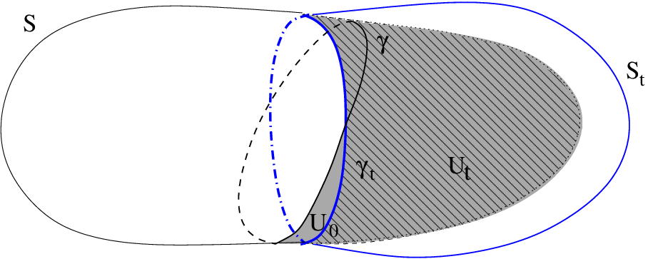
Our next aim is to use this expansion to conclude that the intersection of and near is an embedded curve for all small enough . To do that we will apply the implicit function theorem to the equation . It is useful to introduce a new function , which is still smooth (thanks to (24)) and vanishes at only on the curve . Moreover, its derivative with respect to is nowhere zero on , in fact for all . The implicit function theorem implies that there exist a unique function which solves the equation , for small enough . Obviously, this function is also the unique solution near of for . Consequently, the intersection of and () lying in the neighbourhood of where we are working on is an embedded curve . This curve divides into two connected components (because does). Let us denote by the connected component of which has near (i.e. that lies in the exterior of near ). This connected component in fact lies fully outside of , not just in a neighborhood of , as we see next. First of all, recall that is the boundary of a connected set where is strictly positive. We have just seen that is a continuous deformation of . Let us denote by the domain obtained by deforming when the boundary moves from to (See Fig.3). It is obvious that is obtained by moving first along an amount and the back to by null hypersurfaces. The closed subset of lying outside the tubular neighbourhood where we applied the implicit function theorem is, by construction a proper subset of . Consequently, on this closed set is uniformly bounded below by a positive constant. Given that is the first order order term of the normal variation, all these points move outside of . This proves that is fully outside for sufficiently small . Incidentally this also shows that is a graph over .
The next aim is to show that the outer null expansion of is non-positive everywhere on . To that aim, we will prove that, for small enough , is strictly negative everywhere on . Since is the first order term in the variation of , this implies that the outer null expansion of satisfies for small enough.
By assumption (23), is strictly negative on . Therefore, this quantity is automatically negative in the portion of lying in (in particular, outside the tubular neighbourhood where we applied the the implicit function theorem). The only difficulty comes from the fact that may move outside at some points and we only have information on the sign of on . To address this issue, we first notice that defines a distance function to (because vanishes on and its gradient is nowhere zero). Consequently, the fact that is strictly negative on (by assumption (23)) and that this curve is compact imply that there exists a such that, inside the tubular neighbourhood of , implies . Moreover, the function , which defines , is such that it vanishes at and depends smoothly in . Since takes values on a compact set, it follows that for each , there exists an , independent of such that implies . By taking , it follows that, for , is contained in a -neighbourhood of (with respect to the distance function ) and consequently on this set, as claimed. We restrict to from now on.
Summarizing, so far we have shown that lies fully outside and has . The final task is to use Lemma 3 to construct a weakly outer trapped surface strictly outside . Indeed, the curve divides the locally outermost MOTS in two connected components. Since is locally outermost, there is a two-sided neighbourhood of in . Following the notation in Section 2, we call the interior part of this two-sided neighbourhood. Denote by the complementary of in . By construction, bounds a domain which contains . Now, let be the vector normal to and tangent to that points to the interior of and let be the vector normal to which points to the exterior of . Since lies outside and it is a graph on near , it follows immediately that holds everywhere on . Therefore, Lemma 3 guarantees that there exists a weakly outer trapped surface lying outside , leading to a contradiction. .
Remark. As always, this theorem also holds if all the inequalities are reversed. Note that in this case is defined to be a connected component of the set . For the proof simply take instead of (or equivalently move along instead of ).
Similarly as in the previous section, this theorem can be particularized to the case of conformal Killing vectors, as follows
Corollary 5
Under the assumptions of Theorem 5, suppose that is a conformal Killing vector with conformal factor (including homotheties and isometries ).
Then, there exists such that
If the conformal Killing is in fact a homothety or a Killing vector and it is causal everywhere, the result can be strengthened considerably. The next result extends in a suitable sense Corollary 3 to the cases when the generator is not assumed to be either future or past everywhere. Since its proof requires an extra ingredient we write it down as a theorem
Theorem 6
In a spacetime satisfying NEC and admitting a Killing vector or homothety , consider a locally outermost MOTS in a spacelike hypersurface . Assume that is causal on and that everywhere. Define and assume that this set is neither empty nor covers all of . Then, on each connected component of there exist a point with
Remark. The same conclusion holds on the boundary of each connected components of the set . This is obvious since can be changed to .
Remark. The case , excluded by assumption in this theorem, can only occur if is future or past everywhere on . Hence, this case is already included in Corollary 3.
Proof. We first show that on any point in we have , which has as an immediate consequence that on any point in . The former statement is a consequence of the decomposition , where . The condition that is causal then implies . This can only happen at a point where (i.e. on ) provided there. Moreover, if at any point on the boundary we have , then necessarily the full vector vanishes at this point. This implies, in particular, that the geometric construction of has the property that remains invariant.
Having noticed these facts, we will now argue by contradiction, i.e. we will assume that there exists a connected component of such that everywhere. In this circumstances, we can follow the same steps as in the proof of Theorem 5 to show that, for small enough the surface has a portion lying in the exterior of and which, in the Gaussian coordinates above, is a graph over a subset with is a continuous deformation of . Moreover, the boundary of is a smooth embedded curve . The only difficulty with this construction is that we cannot use everywhere on , in order to conclude that , as we did before. The reason is that there may be points on where . However, as already noted, these points have the property that do not move at all by the construction of , i.e. the boundary (which is the intersection of and ) can only move outside of at points where is strictly negative. Hence on the interior points of we have everywhere, for sufficiently small . Consequently the first order terms in the variation of , namely , is strictly negative on all the interior points of . This implies that has negative outer null expansion everywhere except possibly on its boundary . By continuity, we conclude everywhere. We can now apply Lemma 3 to (where, as before, is the complementary of in ) to construct a smooth weakly outer trapped surface outside the locally outermost MOTS . This gives a contradiction. Therefore, there exists such that , as claimed.
Remark The assumption is a technical requirement for Lemma 3. This is why we had to include an assumption on in Theorem 5 and also that the conclusion of Theorem 6 is stated in terms of the existence of critical points for . If Lemma 3 could be strengthened so as to remove this requirement, then Theorem 6 could be rephrased as stating that any outermost MOTS in a region where there is a causal Killing vector (irrespective of its future or past character) must have at least one point where the shear and the energy “density” along vanish simultaneously.
In any case, the existence of critical points for a function in the boundary of every connected component of and every connected component of is obviously a highly non-generic situation. So, locally outermost MOTS in regions where there is a causal Killing vector or homothety can at most occur under very exceptional circumstances.
Acknowledgments
We are grateful to M. Sánchez, J.M.M. Senovilla and W. Simon for useful comments on the manuscript. We acknowledge financial support under the projects FIS2006-05319 of the Spanish MEC, SA010CO5 of the Junta de Castilla y León and P06-FQM-01951 of the Junta de Andalucía. AC acknowledgments a Ph.D. grant (AP2005-1195) from the Spanish MEC.
References
- [1] Dafermos, M. (2005) Spherically symmetric spacetimes with a trapped surface. Class. Quantum Grav., 22, 2221–2232.
- [2] Bengtsson, I. and Senovilla, J. The boundary of the region with trapped surfaces in spherical symmetry. in preparation.
- [3] Senovilla, J. On the boundary of the region containing trapped surfaces. arXiv: 0812.2767.
- [4] Coll, B., Hildebrandt, S., and Senovilla, J. (2001) Kerr-schild symmetries. Gen. Rel. Grav., 33, 649–670.
- [5] Mars, M. and Senovilla, J. (2003) Trapped surfaces and symmetries. Class. Quantum Grav., 20, L293–L300.
- [6] Senovilla, J. (2003) On the existence of horizons in spacetimes with vanishing curvature invariants. J. High Energy Physics, 11, 046.
- [7] Ashtekar, A. and Galloway, G. (2005) Some uniqueness results for dynamical horizons. Adv. Theor. Math. Phys., 9, 1–30.
- [8] Andersson, L., Mars, M., and Simon, W. (2008) Stability of marginally outer trapped surfaces and existence of marginally outer trapped tubes. Adv. Theor. Math. Phys., 12, 853–888.
- [9] Miao, P. (2005) A remark on boundary effects in static vacuum initial data sets. Class. Quantum Grav., 22, L53–L59.
- [10] Carrasco, A. and Mars, M. (2008) On marginally outer trapped surfaces in stationary and static spacetimes. Class. Quantum Grav., 25, 055011.
- [11] Kriele, M. and Hayward, S. (1997) Outer trapped surfaces and their apparent horizon. J. Math. Phys., 38, 1593–1604.
- [12] Senovilla, J. (2007) Classification of spacelike surfaces in spacetime. Class. Quantum Grav., 24, 3091–3124.
- [13] Andersson, L., Mars, M., and Simon, W. (2005) Local existence of dynamical and trapping horizons. Phys. Rev. Lett., 95, 111102.
- [14] Beem, J., Ehrlich, P., and Markvorsen, S. (1988) Timelike isometries and killing fields. Geom. Dedicata, 26, 247–258.
- [15] Wald, R. (1984) General Relativity. Chicago University Press.
- [16] Senovilla, J. (1997) Singularity theorems and their consequences. Gen. Rel. Grav., 29, 701–848.
- [17] Andersson, L., Mars, M., Metzger, J., and Simon, W. (2009) The time evolution of marginally trapped surfaces. arXiv: 0811.4721.
- [18] Andersson, L. and Metzger, J. (2007) The area of horizons and the trapped region. arXiv: 0708.4252.