Switcher-random-walks: a cognitive-inspired mechanism for network exploration
Abstract
Semantic memory is the subsystem of human memory that stores knowledge of concepts or meanings, as opposed to life specific experiences. The organization of concepts within semantic memory can be understood as a semantic network, where the concepts (nodes) are associated (linked) to others depending on perceptions, similarities, etc. Lexical access is the complementary part of this system and allows the retrieval of such organized knowledge. While conceptual information is stored under certain underlying organization (and thus gives rise to a specific topology), it is crucial to have an accurate access to any of the information units, e.g. the concepts, for efficiently retrieving semantic information for real-time needings. An example of an information retrieval process occurs in verbal fluency tasks, and it is known to involve two different mechanisms: ‘clustering’, or generating words within a subcategory, and, when a subcategory is exhausted, ‘switching’ to a new subcategory. We extended this approach to random-walking on a network (clustering) in combination to jumping (switching) to any node with certain probability and derived its analytical expression based on Markov chains. Results show that this dual mechanism contributes to optimize the exploration of different network models in terms of the mean first passage time. Additionally, this cognitive inspired dual mechanism opens a new framework to better understand and evaluate exploration, propagation and transport phenomena in other complex systems where switching-like phenomena are feasible.
Keywords: random-walks; complex-networks; information retrieval; cognitive systems; switching-clustering;
I Introduction
Semantic memory is a distinct part of the declarative memory system [Tulving 1978] comprising knowledge of facts, vocabulary, and concepts acquired through everyday life [Squire 1987]. Contrary to episodic memory, which stores life experiences, semantic memory is not linked to any particular time or place. In a more restricted definition, it is responsible for the storage of semantic categories and naming of natural and artificial concepts [Budson & Price 2005]. It is known that this memory involves distinct brain regions and its impairment in neurodegenerative diseases such as fronto-temporal dementia [Libon, Xie, Moore, Farmer, Antani, McCawley, Cross, & Grossman 2007], multiple sclerosis [Henry & Beatty 2006] and Alzheimer’s disease [Rogers & Friedman 2008] produce verbal fluency deficits. For this reason, lexical access, the cognitive information-retrieval process in charge of retrieving concepts, has been widely explored through semantic verbal fluency tasks in the context of neuropsychological evaluation [Lezak 1995]. These tests require the generation of words corresponding to a specific semantic category, typically animals, fruits or tools, for a given time. Although the task is easy to explain, it actually results in a complex challenge where retrieving as many concepts as possible in a limited time depends more on cognitive mechanisms than on the knowledge itself. According to the two-component model proposed by A. Troyer [Troyer, Moscovitch, & Winocur 1997], optimal fluency performance involves a balance between two different processes: ‘clustering’, or generating words within a subcategory, and, when a subcategory is exhausted, ‘switching’ to a new subcategory. In the case of naming animals, clustering produces semantically related transitions (e.g. lion-tiger) and switching is a mechanism that allows to jump or shift to different semantic fields (e.g. tiger-shark). While the former is attached to the temporal lobe of the brain, the latter has been associated to a frontal lobe activity [Troyer, Moscovitch, Winocur, Alexander, & Stuss 2002]. Evidences of the interaction between these two regions of the brain during language related tasks has led a number of studies to refer to a fronto-temporal modulation or interaction [Poldrack, Wagner, Prull, Desmond, Glover, & Gabrieli 1999; Troyer, Moscovitch, Winocur, Alexander, & Stuss 2002].
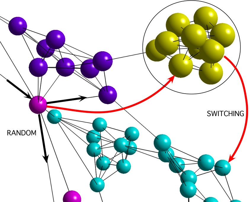
In this paper, the cognitive paradigm that consists of retrieving words from a semantic network [Thornton, Raz, & Tucke 2002; Rogers & Friedman 2008] was generalized to an exploration task on a network. Clustering was modeled as a random-walker constrained to the topology of the network and switching as an extra-topological mechanism that is able to move from any node to any node (see figure 2). The combination of these two processes gave rise to a dual mechanism denoted here as switcher-random-walker (SRW), i.e. a random-walker with the additional ability of switching. The combination of switching and clustering, i.e., free jumping and random walking, was ruled by a parameter , which is the probability of switching at every step, and thus is the parameter that metaphorically rules the fronto-temporal modulation. Therefore the complementary is the probability of clustering at every step, and can be interpreted as the strength of the local perseverance of the exploration before moving somewhere else within the network (specially for those networks with either high clustering coefficient or high modularity). This cognitive inspired paradigm gives rise to the following question: how does switching and its modulation affect random exploration of different network models?
Search, propagation and transport phenomena have been studied in networks [Bollt & Ben-Avraham 2005], where it is crucial to define whether the full topology is known. When it is known, the ease to reach any node from any node is measured by the shortest path length [Watts & Strogatz 1998; B.Tadic & Rodgers 2002]. When it remains unknown, exploration is modeled by random walks along the network [Noh & Rieger 2004]. This is the case of retrieving concepts since the subject is not aware of his full semantic network when naming them. In this kind of cases reachability of nodes is measured with the mean first passage time (MFPT), i.e. the averaged number of steps needed to visit a node for the first time, starting from a node [Snell 1959; Catral, Neumann, & Xu 2005]. Given its relevance in complex media, this paradigm has been recently revisited in a number of studies [Noh & Rieger 2004; Catral, Neumann, & Xu 2005; Condamin, Bénichou, Tejedor, Voituriez, & Klafter 2007].
While different derivations of random-walkers have been recently used to infer the underlying topological properties of complex networks [da Fontoura Costa & Travieso 2007; Ramezanpour 2007; Gómez-Gardeñes & Latora 2008], our aim was to evaluate how SRW (and in particular, the effect of different levels of switching) contributes to the exploration of network models with well known topological properties. Different models which were not necessarily lexico-conceptual architectures were explored by a SRW and its performance was measured by the MFPT (detailed in section II.3). Going back to the cognitive paradigm, retrieving plenty of words in a semantic verbal fluency test not only depends on the number of concepts that the subject knows, but also on an equilibrium between the underlying semantic topology that organizes those concepts and the frequency of switching [Troyer, Moscovitch, & Winocur 1997]. For example, two different studies [Boringa, Lazeron, Reuling, Adèr, Pfennings, Lindeboom, de Sonneville, Kalkers, & Polman 1982; Sepulcre, Vanotti, & et al. 2006] reported that their respective groups of healthy participants produced and animals during seconds. There are two remarkable aspects in these figures. First, participants obviously knew many more animals than those said and, second, there is a high heterogeneity in the number of words. Hence, even though all participants only named a low fraction of the animals they knew, some of them had much more success than others when retrieving them.
II A Markov model of SRW
As introduced in the previous section, our approach for a clustering step consists of a walker unaware of the full network moving from one node to any of its neighbors with no preferential gradients among neighbors. Such exploration task was modeled by the well known random-walker (RW). Switching was implemented as a mechanism where the walker moves to any other node following different probabilistic approaches. Summarizing SRW can be defined as a random- walker with the capability of rendering random shifts.
II.1 Markov Chains
A finite Markov chain is a special type of stochastic process which can be described as follows. Let
| (1) |
be a finite set whose members are the states of the system, which we label . The process moves through these states in a sequence of steps. If at any time it is in state , it moves to a state on the next step with some probability, , where is the set of matrices of non-negative entries where the sum of every row is 1. These probabilities define a square, matrix, :
| (2) |
which we call the matrix of transition probabilities. The importance of matrix theory to Markov chains comes from the fact that the th entry of the th power of , represents the probability that the process will be in state after steps considering that it was started in state . The study of a general Markov chain can be reduced to the study of two special types of chains. These are absorbing chains and ergodic chains (also known as irreducible). The former contain at least one absorbing state, i.e. a state constituted by a proper subset of the whole by which, once entered it cannot be left, and furthermore, which is reachable from every state in a finite number of steps. The latter are those chains where is possible to go from any state to any other state in a finite number of steps and are called regular chains when
For regular chains, the th entry of becomes essentially independent of state as is larger. In the case of regular chains, we can define a stationary probability matrix [Snell 1959] as:
| (3) |
Note that for non regular Markov processes this limit might not exist. For instance .
The matrix consists of a row probability vector which is repeated on each row. This vector can be obtained as the only probability vector satisfying [Grinstead & Snell 1952]. For the case of regular Markov processes obtained from random walks on graphs, this indicates that in the long run, the probability to be in a node is independent of the node where the process started.
II.2 Graph Characterization
This section is devoted to the characterization of the underlying object over which we apply our algorithm of exploration, a graph. Beyond its main features, we discuss the consequences of connectedness in order to clearly define the frameworks over which the SRW algorithm can be defined. Finally, we briefly define the graph models studied numerically in section III.

Let us suppose that our Markov chain is defined by some graph topology. A graph is defined by a set of nodes, , and a set of links , being a subset of . In our approach, the graph is undirected and we avoid the possibility that a node contains auto-loops or that two links are connecting the same nodes. The size of the graph is , i.e. the cardinal of the set of vertices. Its average connectivity is defined as:
| (4) |
The topology of our graph is completely described by a symmetrical, matrix, , the so-called adjacency matrix, whose elements are defined as:
The connectivity of the node , is the number of links departing from and it can be easily computed from the adjacency matrix as:
| (8) |
Following the characterization, we now define the degree distribution, which is understood as the probability that a randomly chosen node displays a given connectivity. In this way, we define the elements of such a probability distribution, as:
| (9) |
The above defined measures are the identity card of a given graph . One could think that it is enough because our main goal is to describe and characterize an exploration algorithm over . However, specially in the models of random graphs, we cannot be directly sure that our adjacency matrix defines a fully connected graph, i.e, that there exists, with probability a path from any node to any node . In deterministic graphs, we can solve this problem by assuming, a priori, that our combinatorial object is fully connected. Furthermore, we could agree that, when performing rewirings at random, we impose the condition of connectedness. The case of pure random graphs is a bit more complicated. Indeed, a random graph is obtained by a stochastic process of addition or removal of links [Bollobas 2001]. Thus, we need a criteria to ensure that our graph is connected or, at least, to work over the most representative component of the obtained object. Full connectedness is hard to ensure in a pure random graph. Instead, what we can find is a giant connected component, . Informally speaking, we can imagine an algorithm spreading at random links among a set of predefined nodes, the so-called Erdös-Rényi graph process. The growing graph displays, at the beginning, a myriad of small clusters of a few nodes and, when we overcome some threshold in the number of links we spread at random, a component much bigger than the others emerges, i.e. the [Erdös & Rényi 1960]. In this way, M. Molloy and B. Reed [Molloy & Reed 1995] demonstrated that, given a random graph with degree distribution , if
| (10) |
then, there exists, with high probability, a giant connected component. The first condition we need to assume is thus, that the studied graphs satisfy inequality (10). Beyond this assumption, we impose the following criteria when studying our model networks:
- 1.
In a deterministic graph (for example, a chain or a lattice) where we perform random re-wirings, we do not allow re-wirings that break the graph.
- 2.
If a graph is the result of an stochastic process, the exploration algorithm is defined only over the (this could imply the whole set of nodes).
- 3.
The adjacency matrix is the adjacency matrix of the . We remove the nodes that, in the beginning, participated in the process of construction of but fell outside the .
All the model graphs studied in this work satisfy the above conditions.
In order to enable useful comparative analysis, we built different networks, all of them with nodes and links. The results were averaged after instances per network model. Let us briefly define the models we will study with our exploration algorithm.
Watts-Strogatz Small-World Network. We built an annulus with nodes in such a way that every node is connected to different nodes (2000 undirected links) [Watts & Strogatz 1998]. Once the annulus was constructed, every link suffered a random re-wiring with connectivity .
Erdös Rényi Graph. Over a set fo nodes we spread at random links, avoiding duplication and self-interaction. It can be shown that the obtained graph displayed a binomial degree distribution [Erdös & Rényi 1960]:
| (11) |
being the probability of two nodes being connected. Its value corresponds to
| (12) |
Random-Modular. We built different components of nodes and links, spread at random (as explained for Erdös Rényi graphs) among the nodes of every component. In this case, we ensure connectedness of such components. Once the ten components are constructed, every link suffers a random rewiring with a node either from the same component or not, with probability .
Preferential Attachment. We provide a seed of connected nodes. Every new node was connected to of the existing nodes with probability proportional to the connectivity of the existing nodes, i.e., suppose that, at time a new node comes in to the graph. At this time step, the graph will display an adjacency matrix .
| (13) |
where
| (14) |
This operation is repeated in an iterative fashion (i.e., updating ) times per node. It can be shown that, at the limit of a large number of nodes the outcome of this algorithm generates a graph whose degree distribution is a power law [Barabasi & Albert 1999]:
| (15) |
with . It is worth noting that such an algorithm avoids the possibility of unconnected components.
II.3 Random walk over a graph as a Markov Process
In this framework, the transition from node to is just the probability that a random-walker starts from some node and reaches the node , after some steps. Consistently, the probability that being in we reach the node in a single step (i.e, ) is:
| (16) |
This is the general form for a Markov formalization of a random-walker within a graph defined by its adjacency matrix . Throughout this work we assume that our graphs define regular Markov processes (see section II.1). Under the above definition of , regularity is assured if and only if the graph is not bipartite (i.e., it contains, at least, one loop containing an odd number of nodes). To see that bipartite graphs are not regular, it is enough to notice that for any pair of nodes there are only either odd or even paths joining them, but not both. Hence if then and therefore the process cannot be regular.
Summarizing, despite that connectedness ensures that the process is ergodic,
it does not ensure regularity and therefore the might not exist. The existence of an odd loop breaks such parity problem and enables to stabilize to a specific matrix of stationary probabilities when . Thus, we must impose another assumption to our studied graphs: Our algorithm works over non-bipartite graphs which satisfy the criteria imposed in section II B. It is straightforward to observe that, if the assumption of regularity holds, the above Markov process has a stationary state with associated probabilities proportional to the connectivity of the studied node [Noh & Rieger 2004]:
| (17) |
From now on, we will refer to the transition matrix above defined as , since it denotes the probabilities of the movements related to clustering.
II.4 Switcher-random-walker
In the retrieval model introduced here, the matrix of transition probabilities is a linear combination of the switching transition probabilities and the clustering transition probabilities , as defined in the above section. The Markov process is a switcher-random-walker and the states represent the location of such walker in the network.
The matrix is ergodic and regular since all entries are strictly greater than zero, and has equal rows, i.e. constant columns. The reason is that the probability of reaching a node through switching is independent of the source node . In this way, we could consider that we define a scalar field over the nodes of the graph:
| (18) |
Consistently,
| (19) |
We can define this field in many different ways. As the more representative, we revise several scalar fields that can provide us interesting information about the process:
| (20) |
In the first and most simple case switching to any other node is a random uniform process, and we refer to this process as uniformly distributed switching. The second case corresponds to the situation where the probability to reach a given node through switching is proportional to its connectivity, which we call positive degree gradient switching. The last one assumes that is and corresponds to the situation where the switcher jumps with more probability to weakly connected nodes, and we refer to it as negative degree gradient switching. These three variants of switching were studied when combined with a random-walker within the above graph topologies (see fig.(3)). They were denoted by , and respectively.
The matrix defined in the above section is ergodic and regular but restricted to the transitions allowed by the adjacency matrix of the network of study. We modeled as equi-probable the transitions among linked nodes of the network. Hence the probability of moving from a node to a a node through clustering for a given graph with an adjacency matrix , is
| (21) |
Thus, is defined as:
| (22) |
where is the probability of switching. Consistently, the entries of are given by:
| (23) |
We observed that is also ergodic and regular. This follows from the fact that has already all entries strictly greater than zero, and thus will have all entries greater than zero for any . For the case of , is just which we assumed to be regular.
Among other interesting descriptive random variables that can be evaluated for regular chains, the matrix of the mean first passage time (MFPT) is a matrix , crucial for measuring the retrieval or exploratory performance of any stochastic strategy; the MFPT needed to go from a node to a node is denoted by [Noh & Rieger 2004] and represents the time (in step units) required to reach state for the first time starting from state . It is important to note that is not necessarily equal to , i.e. it might happen that the time required to go from state to state is different to the time required to go from state to state .
In order to obtain the analytical expression of MFPT, we must define first a fundamental matrix [Grinstead & Snell 1952] which is given by
| (24) |
where
| (25) |
and is the identity matrix of size .
In this case the entry of can be understood as a measure of the deviations of the th entry of from their limiting probabilities , which, as commented in section II.1, is any of the equal rows of . From and we can obtain the analytical derivation of (for more details see [Grinstead & Snell 1952]):
| (26) |
Finally, we denote as the averaged value of all entries for a switcher random walker exploring a network . Since it is not necessarily symmetrical, we must take into account all the entries outside the main diagonal. The main diagonal was not taken into account, since it represents the returning time, which we do not consider as a part of the exploration of the net. Thus,
| (27) |
This measure provides a general evaluation of how reachable is, on average, any node from any other node in a specific network using a switcher random-walker. It is interesting to notice that such measure has an upper bound which is precisely the size of the net. Indeed, let us suppose we have a clique of size , i.e., a graph, , where equals and every node is connected to itself and to all remaining nodes. It corresponds to the case where the probability of switching is . Let be a random variable whose outcomes are such that, :
| (28) |
We define a stochastic process, namely, the realizations of through different time steps, Let us define another random variable, , namely the number of realizations of needed to ensure that there has been one realization of equal to :
| (29) |
Clearly, and due to the symmetry of our experiment, all the nodes behave in the same way. Furthermore,
| (30) |
i.e., we need, in average realizations of in order to obtain, at least, one realization , . We observe that the above random experiment is exactly a random switching over a graph containing nodes, and that is the of this process. Let us suppose we have a . This implies that, in average
| (31) |
which is a contradiction, since the graph has nodes. Thus, for a given graph :
| (32) |
This value represents an horizontal asymptote in the model of SRW as increases, and it is clearly defined in our model experiments (see figure 3).
III Results and discussion
Our main result was that SRW exploration, a cognitive inspired strategy that combines random-walking with switching for random exploration of networks, decreased the of all models for all SRW variants. This means that, on average, the number of steps needed to travel between every pair of nodes decreases and thus the overall exploration abilities of a SRW within the networks improves respect to RW.
Regarding (Fig. 3A), exploration performance of random-modular and small-world networks severely improves, overtaking scale-free at . Moreover, at all the networks but scale-free converged, leading to a remarkable scenario where modularity and high clustering coefficients are not topological handicaps for an efficient information retrieval.
Switching in severely improves in modular and small-world networks while hardly decreases it in scale-free and random. The reason is that a random-walker on both kind of networks already shows a gradient to visit highly connected nodes [Noh & Rieger 2004], and a positive-degree switching supported rather than compensated this effect due to redundancy on hubs 3B).
In , intermediate values of q (around for all but scale-free models) showed optimal performance with a similar effect to the one produced by . However, it only partially succeeded in compensating the already commented natural RW gradient for hubs. (Fig. 3C). Interestingly, those values close to produced an inverse situation where hubs are so unlikely to be reached that the overall exploration performance decreased for all the models but dramatically for scale-free model, where the degree heterogeneity is specially high. On the contrary, small-world model showed a very similar performance when explored by any of the three SRW variants. The reason is that in this model, the degree distribution is very homogeneous, and thus different degree gradients of switching produced very little differences.
The approximate convergence of the exploration efficiency (for most of the topologies when using or with a moderate switching rate) allows a system to organize information or to evolve without compromising exploration and retrieval efficiency. In this sense, semantic memory might be organizing information in a strongly modular or locally clustered way without compromising retrieval performance of concepts. In a more general perspective, the addition of a switching mechanism and its interaction with random-walker dynamics opens a new framework to understand processes related to information storage and retrieval. Indeed, switching not only mitigates exploration deficits of certain network topologies but also might provide certain robustness to the system. For instance, the rewired links (known as short-cuts) in both small-world and random-modular models are contributing to facilitate access to different regions of the network. Those short-cuts might compensate a switching impairment or dysfunction and vice versa, i.e. switching would ensure an accurate exploration of the network even though a targeted attack removed those short-cuts permanently.
Similar mechanisms to switching have been observed in the context of information networks. In particular, the iterative algorithm PageRank estimates a probability distribution used to represent the likelihood that a person randomly clicking on links will arrive at any particular page for a hyper-linked set of documents (e.g. the world-wide-web) [Brin & Page 1998]. The user is supposed to be a random-surfer who begins at a random web page and keeps clicking on links but never hitting back. The damping-factor is an additional item that includes the fact that the user can get bored and start on another random page. The combination of these two processes is used by the Google Internet search engine to estimate the relevance of different links (PageRank values). Interestingly, while the objective (rank link targets) and the framework (hyper-linked documents, i.e. directed graphs) are not the same, the cognitive-inspired SRW described here and PageRank algorithm combine random-walks restricted to a topology with an extra-topological mechanism in order to evaluate tasks in complex networks.
The model proposed here could have implications in other systems that usually have a conflict between organization and retrieval or spreading efficiency. It will be object of further studies in other phenomena unrelated to cognitive processes such as infection epidemiology, information spreading or energy landscapes.
Acknowledgments
JG is a fellow of the Government of Navarra. IM is a fellow of the Caja Madrid Foundation. This work was supported by James McDonnell Foundation to BCM, MEC of Spain BFM2006-03036 to SAT and the European Commission (NEST-Pathfinder: ComplexDis contract number: 043241) to PV. Thanks to Ricard V. Solé for his useful comments and support in the design of figures.
References
- Barabasi & Albert [1999] Barabasi, A.-L., & Albert, R. (1999). Emergence of scaling in random networks. Science, 286, 509–512.
- Bollobas [2001] Bollobas, B. (2001). Random Graphs. Cambridge University Press.
- Bollt & Ben-Avraham [2005] Bollt, E. M., & Ben-Avraham, D. (2005). What is special about diffusion on scale-free nets? New Journal of Physics, 7, 26–47.
- Boringa et al. [1982] Boringa, J., Lazeron, R., Reuling, I., Adèr, H., Pfennings, L., Lindeboom, J., de Sonneville, L., Kalkers, N., & Polman, C. (1982). The brief repeatable battery of neuropsychological tests: normative values allow application in multiple sclerosis clinical practice. Multiple Sclerosis, 7(4), 263–267.
- Brin & Page [1998] Brin, S., & Page, L. (1998). The anatomy of a large-scale hypertextual web search engine. Proceedings of the seventh international conference on World Wide Web, 7, 107–117.
- B.Tadic & Rodgers [2002] B.Tadic, & Rodgers, G. (2002). Packet transport on scale free networks. Advances in Complex Systems, 5, 445–456.
- Budson & Price [2005] Budson, A. E., & Price, B. H. (2005). Memory dysfunction. The New England Journal of Medicine, 352(7), 692–699.
- Catral et al. [2005] Catral, M., Neumann, M., & Xu, J. (2005). Matrix analysis of a markov chain small-world model. Linear Algebra and its Applications, 409, 126–146.
- Condamin et al. [2007] Condamin, S., Bénichou, O., Tejedor, V., Voituriez, R., & Klafter, J. (2007). First-passage times in complex scale-invariant media. Nature, 450(7166), 77–80.
- da Fontoura Costa & Travieso [2007] da Fontoura Costa, L., & Travieso, G. (2007). Exploring complex networks through random walks. Physical Review E, 75(016102).
- Erdös & Rényi [1960] Erdös, P., & Rényi, A. (1960). On the evolution of random graphs. Publ. Math. Inst. Hung. Acad. Sci, 5, 17–61.
- Gómez-Gardeñes & Latora [2008] Gómez-Gardeñes, J., & Latora, V. (2008). Entropy rate of diffusion processes on complex networks. Physical Review E, 78, 065102.
- Grinstead & Snell [1952] Grinstead, C. M., & Snell, J. L. (1952). Markov chains. In AMS (Ed.) Introduction to probability. AMS.
- Henry & Beatty [2006] Henry, J., & Beatty, W. (2006). Verbal fluency deficits in multiple sclerosis. Neuropsychologia, 44, 1166–1174.
- Lezak [1995] Lezak, M. (1995). Neuropsychological assessment. 3rd edition. New York: Oxford University Press.
- Libon et al. [2007] Libon, D., Xie, S., Moore, P., Farmer, J., Antani, S., McCawley, G., Cross, K., & Grossman, M. (2007). Patterns of neuropsychological impairment in frontotemporal dementia. Neurology, 68, 369–375.
- Molloy & Reed [1995] Molloy, M., & Reed, B. A. (1995). A critical point for random graphs with a given degree sequence. Random Structures and Algorithms, 6, 161–180.
- Noh & Rieger [2004] Noh, J. D., & Rieger, H. (2004). Random walks on complex networks. Physical Review Letters, 92(11), 118701.
- Poldrack et al. [1999] Poldrack, R., Wagner, A., Prull, M., Desmond, J., Glover, G., & Gabrieli, J. (1999). Functional specialization for semantic and phonological processing in the left inferior prefrontal cortex. Neuroimage, 10(1), 15–35.
- Ramezanpour [2007] Ramezanpour, A. (2007). Intermittent exploration on a scale-free network. Europhysics Letters, 77, 60004.
- Rogers & Friedman [2008] Rogers, S. L., & Friedman, R. B. (2008). The underlying mechanisms of semantic memory loss in alzheimer’s disease and semantic dementia. Neuropsychologia, 46(1), 12–21.
- Sepulcre et al. [2006] Sepulcre, J., Vanotti, S., & et al., R. H. (2006). Cognitive impairment in patients with multiple sclerosis using the brief repeatable battery-neuropsychology test. Multiple Sclerosis, 12, 187–195.
- Snell [1959] Snell, J. L. (1959). Finite markov chains and their applications. The American Mathematical Monthly, 66(2), 99–104.
- Squire [1987] Squire, L. (1987). Memory and Brain. New York: Oxford University Press.
- Thornton et al. [2002] Thornton, A., Raz, N., & Tucke, K. (2002). Memory in multiple sclerosis: contextual encoding deficits. Journal of International Neuropsychology, 8(3), 395–409.
- Troyer et al. [1997] Troyer, A. K., Moscovitch, M., & Winocur, G. (1997). Clustering and switching as two components of verbal fluency: Evidence from younger and older healthy adults. Neuropsychology, 11(1), 138–146.
- Troyer et al. [2002] Troyer, A. K., Moscovitch, M., Winocur, G., Alexander, M., & Stuss, D. (2002). Clustering and switching on verbal fluency: the effects of focal frontal- and temporal-lobe lesions. Neuropsychologia, 40(5), 562–566.
- Tulving [1978] Tulving, E. (1978). Episodic and semantic memory. In Organization and memory, (pp. 381–403). New York and London: Academic Press.
- Watts & Strogatz [1998] Watts, D., & Strogatz, S. (1998). Collective dynamics of ’small-world’ networks. Nature, 4(393), 440–442.