When all the quartic couplings between $H_{1}$ and $H_{2}$ vanish (except $\lambda_{5}$ which we take tiny but non vanishing to avoid the direct detection problem above), all states are degenerate at tree-level. At one-loop, the neutral states remain exactly degenerate due to the Peccei-Quinn symmetry, up to the very small $\lambda_{5}$ contribution, and a splitting $m_{H^{+}}-m_{H_{0}}\simeq 350$ MeV is induced between the charged and the neutral states[25]. Because of the smallness of these splittings for the annihilation cross-section, it is a very good approximation to consider all states as exactly degenerate and all quartic couplings as vanishing. In this limit, the DM species (co)annihilate into either known gauge bosons or fermions through an intermediate gauge boson. The corresponding Feynman diagrams are shown in Fig. 10 and Fig. 12 of the Appendix B. The only free parameter is the DM mass, so that there is a one-to-one correspondence between the DM mass and the relic density.

Let $\sigma_{0}\simeq A_{0}/v+B_{0}\,v$ be the effective cross-section in this limit, it is given by the average of the cross-sections for all the annihilation and coannihilation processes relevant for the relic density calculation. We obtain, at leading order,

where $\alpha_{2}=g^{2}/4\pi$ is the weak coupling constant, $s_{w}\equiv\sin\theta_{W}$, and $c_{w}\equiv\cos\theta_{W}$. The zero velocity term $A_{0}$ agrees with the result for $n=2$ of Eq. (12) in Ref. [25], up to a factor one half²² 2 The extra factor $1/2$ in Ref. [25] could be due to a convention in the definition of the thermal average.. The velocity dependent term is mainly due to coannihilations, its coefficient $B_{0}$ is of the same order of magnitude as $A_{0}$. The analytical expression for $B_{0}$ will not be given here, but we took it into account in numerical evaluations.

It is interesting to notice that all the (co)annihilation cross-sections fall as $m_{H_{0}}^{-2}$, as required by unitarity constraints. For annihilations into gauge bosons, this behavior is achieved after the cancellation of various diagrams whose amplitudes are connected by gauge invariance. Let us for instance examine in more details the process $H_{0}H_{0}\rightarrow ZZ$. Naively, the contribution from the longitudinal modes $Z_{L}$ to the amplitude is enhanced by a factor $m_{H_{0}}^{2}/m_{Z}^{2}$ compared to the contribution from the transverse modes $Z_{T}$. This would lead to an unacceptable behavior of the cross-section, $\sigma\sim m_{H_{0}}^{2}$. Actually, a cancellation of the longitudinal parts occurs between the $t$ and the $u$-channels on one hand, and the point-like interaction diagram (”$p"-$channel) on the other hand. Notice that the $t$ and the $u$-channels involve the propagator of $A_{0}$. When quartic couplings vanish, all DM states are degenerate, so that this cancellation is almost exact in the sense that the residual amplitude to longitudinal modes is given by

For the two transverse modes, there is no cancellation, their amplitude amounts to

In the high mass regime, ${\cal M}_{L}\ll{\cal M}_{Ti}$. For e.g. $m_{H_{0}}\simeq 550$ GeV, ${\cal M}_{L}/{\cal M}_{Ti}\simeq 1.4~\%$. As $\sigma(H_{0}H_{0}\rightarrow ZZ)\propto\Sigma_{i}|{\cal M}_{Ti}|^{2}+|{\cal M}_{L}|^{2}$, we see that the residual longitudinal amplitude is totally negligible. Therefore, in the pure gauge limit, gauge bosons produced by the annihilations of $H_{0}$ are almost purely transverse.

In Fig. 1, we have plotted the DM relic density as a function of mass, assuming zero quartic couplings between $H_{1}$ and $H_{2}$. The solid and the dashed curves correspond to the instantaneous freeze-out approximation with and without velocity dependent terms in $\langle\sigma v\rangle$. As can be seen, these terms shift down the value of $\Omega_{\rm DM}h^{2}$ by only $\sim 4\%$. Also shown are more exact points from a full integration of the Boltzmann equation, obtained with the MicrOMEGAs program [39]. The latest 5-years WMAP results, combined with baryon acoustic oscillations and supernovae data yield $\Omega_{\rm DM}h^{2}=0.1131\pm 0.0034$ [40]. We see that, in the absence of quartic couplings, the DM mass is determined by the relic density,

in agreement with the results of Ref. [25], up to the update of $\Omega_{\rm DM}h^{2}$. At $3\sigma$ the DM mass cannot be lighter than $508$ GeV. It is worth noticing that the value of $m_{H_{0}}$ is quite sensitive to the precision at which $\Omega_{\rm DM}h^{2}$ is determined. Also, the approximate solid curve from Fig. 1 gives a slightly higher mass range, $m_{H_{0}}=553\pm 8.5$ GeV. The discrepancy is attributable to the instantaneous freeze-out approximation rather than to the values of the cross-sections in Eq. (25).

When the scalar quartic couplings between $H_{1}$ and $H_{2}$ are switched on, the cross-section is affected in two ways. First, non-zero mass splittings between members of the inert doublet, Eq. (6) will modify the amplitude of pure gauge diagrams of both annihilation and coannihilation processes. Second, a series of new annihilation and coannihilation processes which involve the usual Higgs particle appear, see Fig. 12 of the Appendix B.

It is instructive to analyze how cross-sections grow with the quartic couplings. As a generic example, let us consider again the process $H_{0}H_{0}\rightarrow ZZ$. When a non zero mass splitting between $H_{0}$ and $A_{0}$ exists, the amplitudes to longitudinal modes from the $t$, $u$ and $p$-channels do not cancel exactly anymore and is not suppressed anymore by a $m^{2}_{Z}/m^{2}_{H_{0}}$ as in Eq. (26). Instead, a contribution proportional to $(m_{A_{0}}^{2}-m_{H_{0}}^{2})$ remains (in the high-mass regime squared mass splittings are small with respect to $m^{2}_{H^{0}}$ but not necessarily with respect to $m^{2}_{Z}$, as we will see),

Furthermore, there is also a new contribution from the Higgs exchange in the $s$-channel $H_{0}H_{0}\rightarrow h^{*}\rightarrow ZZ$. The amplitude of the $s$-channel is proportional to $\lambda_{H_{0}}v_{0}^{2}=(m_{H_{0}}^{2}-\mu_{2}^{2})$. When added to the $t$, $u$ and $p$-channels, a further cancellation takes places, and the total amplitude to longitudinal modes due to quartic couplings is finally given by

to be compared with Eqs. (26-27). Corrections to transverse modes are negligible, because they are smaller by a factor $m_{Z}^{2}/m_{H_{0}}^{2}$. Therefore, gauge bosons produced by the scalar quartic couplings are almost purely longitudinal in the high mass regime, whereas those from the gauge interactions alone are almost purely transverse. As a consequence, the annihilation cross-section can only grow (if we neglect the tiny residual amplitude of Eq. (26)) when scalar quartic couplings are switched on. The scalar coupling contribution to the cross-section $\sigma(H_{0}H_{0}\rightarrow ZZ)$ becomes comparable to the gauge one for $\lambda_{A_{0}}\simeq g^{2}/(2\sqrt{2}c_{w}^{2})\simeq 0.2$. This corresponds to a small value of the splitting $|m_{A_{0}}-\mu_{2}|\sim m_{W}^{2}/\mu_{2}$.

The above analysis for the process $H_{0}H_{0}\rightarrow ZZ$ serves as a demonstration that the various (co)annihilations cross-sections can only grow with the splittings between $\mu_{2}$, $H_{0}$, $A_{0}$ and $H_{c}$ ($H_{c}$ stands for $H_{\pm}$). To further check this conclusion, we will make use of an expansion of the cross-sections that is valid in the asymptotic high-mass regime we consider here. The cross-sections are simultaneously expanded in $m^{2}_{W,Z,h}/m^{2}_{H_{0}}$ and in $\lambda_{H_{0},A_{0},H_{c}}v_{0}^{2}/m_{H_{0}}^{2}$ (except maybe for the top quark, the corrections induced by the fermion masses of the SM are really negligible in this regime). The orders of magnitude of these parameters which give the correct relic abundance will serve as an a posteriori justification for the use of this expansion, as we will see. We separate the various inclusive (co)annihilation cross-sections into $\lambda$ independent and $\lambda$ dependent terms as

with $\{i,j=0,1,2,3\}$ corresponding to $\{H_{0},A_{0},H^{+},H^{-}\}$. Only the expressions of the dominant velocity independent terms will be given here. To leading order, for $\sigma_{0}^{ij}$, we have

The $\lambda$ dependent cross-sections can be written in a compact way as

with the coefficients $\Lambda^{ij}=\Lambda^{ji}$ given by

As we can see, the cross-sections $\sigma^{ij}$ can only increase when the scalar quartic couplings are switched on. The values of the $\lambda$ corresponding to a constant cross-section $\sigma^{00}$ (or $\sigma^{11}$) lie on an ellipsoid. For the others $\sigma^{ij}$, the ellipsoid is degenerate in a cone ($\Lambda^{02}$ or $\Lambda^{23}$), or in a plane ($\Lambda^{22}$). We can notice in Eq. (34) that the coannihilations cross-sections $\sigma_{\lambda}^{01}$, $\sigma_{\lambda}^{02}$ and $\sigma_{\lambda}^{12}$ are determined by the mass splittings between $H_{0}$, $A_{0}$ and $H_{c}$, while the annihilation cross-sections $\sigma_{\lambda}^{00}$, $\sigma_{\lambda}^{11}$ and $\sigma_{\lambda}^{23}$ also depend on the splitting between $H_{0}$, $A_{0}$, $H_{c}$ and the scale $\mu_{2}$.

From the positivity of the coefficients $\Lambda^{ij}$ in Eq. (34), we can expect that the relic density will decrease when the quartic couplings are turned on. As shown by the instantaneous freeze-out approximation, the final relic abundance is actually controlled by the effective thermal cross-section Eq. (19), where Boltzmann suppression factors $e^{-(m_{i}-m_{0})/T}$ appear when the mass splittings differ from zero. The net result between this thermal damping effect and the rise of each cross-section with $\lambda$ turns out to be positive. Therefore, even in the presence of non zero scalar couplings, the lower bound $m_{H_{0}}\geq m^{*}$ for the relic density, with

remains valid. Above this threshold, the scalar coupling contribution to the cross-section has to become progressively dominant over the gauge one in order to obtain the correct relic density set by WMAP. It can be seen from Fig. 1 or Eq. (25) that both contributions become equal for $m_{H_{0}}\simeq\sqrt{2}m^{*}=755$ GeV. For $m_{H_{0}}\geq 1.7$ TeV, the gauge contribution falls below 10%.

For a given mass $m_{H_{0}}$, it is clear that the values of the quartic couplings that are compatible with WMAP are bounded. As we will see, due to Eq. (34), they form approximately an ellipsoid in the parameter space $\{\lambda_{H_{0}},\lambda_{A_{0}},\lambda_{H_{c}}\}$. Mass splittings are also limited, because

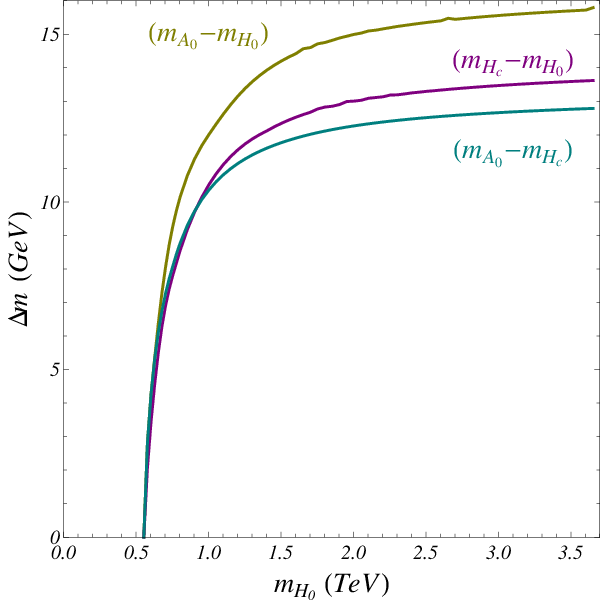
Upper bounds for each $|\lambda|$ and for each mass splitting are shown in Fig. 2, as a function of $m_{H_{0}}$. We see that large values of $\lambda\simeq{\cal O}(1)$ are permitted, the upper bound for each $\lambda$ (or a linear combination of them) grows linearly with the DM mass when $m_{H_{0}}\gg m^{*}$. We have noticed earlier that the coannihilation cross-sections are determined by the mass splittings. It turns out that coannihilations involving the charged component are stronger for a given mass splitting. This explains why the maximum mass splittings between $H_{c}$ and $H_{0}$ (or $A_{0}$) are slightly smaller than the maximum splitting $m_{A_{0}}-m_{H_{0}}$. Also the maximum $m_{H_{c}}-m_{H_{0}}$ is larger than the maximum $m_{A_{0}}-m_{H_{c}}$ because we have assumed that $H_{0}$ is the lightest DM particle. As $\Delta m_{ij}\simeq(m_{i}^{2}-m_{j}^{2})/2\mu_{2}\simeq(\lambda_{i}-\lambda_{j})v_{0}^{2}/2m_{H_{0}}$ and $\lambda_{i}-\lambda_{j}\propto m_{H_{0}}$ for $m_{H_{0}}\gg m^{*}$, each mass splitting is bounded by an asymptotic value. Numerically, we find

These small splittings serve as an a posteriori justification of the pertinence of the joint expansion in $m^{2}_{W,Z,h,f}/m^{2}_{H_{0}}$ and in $\lambda_{H_{0},A_{0},H_{c}}v_{0}^{2}/m_{H_{0}}^{2}$ we made. They also imply that corrections to EWPT observables are negligible in the high mass regime of the IDM (see Eq. (8)).

On Fig. 3, two sections in the parameter region allowed by WMAP are shown for three values of the DM mass $m_{H_{0}}=600,\,1000,\,3000$ GeV, they correspond to the two cases $m_{A_{0}}=m_{H_{0}}$ and $m_{H_{c}}=(m_{A_{0}}+m_{H_{0}})/2$. The contours were obtained using the instantaneous freeze-out approximation and for a $1\sigma$ variation of $\Omega_{\rm DM}h^{2}$. We have checked that the results agree very well with the output of MicrOMEGAs. Ellipsoidal contours are superimposed on these figures in red dashed line. They correspond to an expansion in terms of $\Delta m_{ij}/T$ up to quadratic terms of the Boltzmann exponential factors in the effective thermal cross-section. This ellipsoidal approximation is not accurate when the mass splittings are not negligible compared to the temperature around freeze-out, as can be seen for example in the right panel of Fig. 3 when $m_{H_{0}}=600$ GeV.

We can conclude that the relic abundance required by WMAP can be naturally achieved in the large mass regime of the inert doublet model. A viable DM candidate with a mass in the multi-TeV range only requires at least one of the scalar quartic couplings to be of order 1. In this case, there is no need for any fine-tuning in the parameters of the lagrangian. Moreover, the relic density constraint does not put a lower bound on any of the quartic couplings (or a linear combination of them). For any value of the DM mass above the limit of Eq. (28), one or two of them can even be zero accidentally or if some symmetry is added to the model.

The growth of the values of $\lambda$ with mass as needed by WMAP imposes an upper bound on the mass of the DM candidate because of unitarity considerations. If we require all the physical quartic couplings $\lambda_{H_{0}}$, $\lambda_{A_{0}}$ and $\lambda_{H_{c}}$ in Eq. (2) to be smaller than $4\pi$, we get the bound

while for $2\pi$ instead of $4\pi$ we get $m_{H_{0}}<30$ TeV. This is in agreement with the general unitarity bound which holds on any thermal DM relic whose relic density proceed from the freeze-out of its annihilation [41].

We have shown that the inert doublet model in the high mass regime can provide a viable DM candidate for a very large range of the DM mass. However, for large masses above $\sim 5$ TeV, the freeze-out will occur before the onset of the electroweak phase transition. In this case, all DM components have the same mass $m_{0}=\mu_{2}$ at the epoch of freeze-out, so that deviations from the previous analysis are expected. They annihilate into components of the usual Higgs doublet $H_{1}$ in the unbroken phase. The threshold between the unbroken and the broken phases occurs at a temperature $T_{c}\simeq 200$ GeV. Although the electroweak phase transition in the SM is second order the phase transition, it occurs rather quickly (see e.g. [42] and Refs. therein) and for simplicity we will assume a sharp threshold for the freeze-out of our DM candidate. This means that the freeze-out will be assumed to be in the broken (unbroken) phase for $m_{H_{0}}\leq(>)5$ TeV.

In the unbroken phase, the scalar coupling part of the effective annihilation cross-section relevant for the relic density is modified as³³ 3 We assume that all the components of the Higgs doublet have masses much smaller than $m_{0}$.

the pure gauge part of the cross-section is still given by Eq. (25), in the limit $s_{w}\rightarrow 0$. The WMAP constraint determines $r_{\lambda}$, we get

Note that $r_{\lambda}=4\pi$ for $m_{0}=46$ TeV and $r_{\lambda}=2\pi$ for $m_{0}=22.5$ TeV. The DM mass range is therefore slightly reduced.

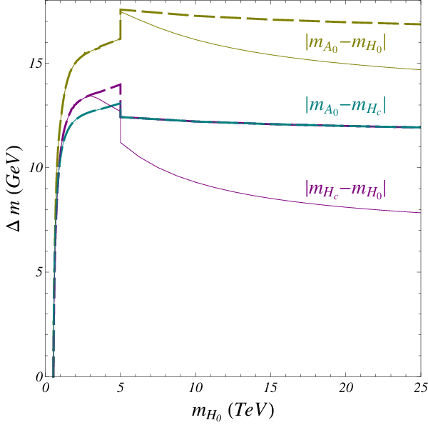
The maximal values of the scalar quartic couplings and the mass splittings allowed by WMAP corresponding to a freeze-out in the unbroken phase are shown in Fig. 4. We see that $|\lambda_{H_{0}}|$ and $\lambda_{A_{0}}$ are increased while $\lambda_{H_{c}}$ is reduced. However, if the stability conditions are taken into account, the maximum of $|\lambda_{H_{0}}|$ is given by the positive branch $\lambda_{H_{0}}>0$ which is smaller. Also, the maximum mass splitting $|m_{H_{0}}-m_{A_{0}}|$ can be slightly higher if the freeze-out occurs during the unbroken phase of the SM. We get

Finally, as it can be seen on Fig. 4, the vaccum stability conditions affect significantly the maximal values of $|m_{A_{0}}-m_{H_{0}}|$ and $|m_{H_{c}}-m_{H_{0}}|$.

It is worth emphasizing that the stability conditions do not constrain the mass range of the DM candidate. To fulfill them, it suffices for $\lambda_{3}$ to be positive and larger in absolute value than $\lambda_{4}+\lambda_{5}$. Therefore, these conditions do not put a stringent constraint on the possibility of having a very heavy DM candidate with the correct relic abundance.

In the following we consider only the case of real multiplets. As explained in section 2.2, for complex multiplets one just must divide the mass obtained with a real multiplet by $\sqrt{2}$. At tree-level, all the components of a real multiplet have the same mass $m_{0}$. As the mass splittings induced at one-loop are very small (see Eq. (15)), it is a very good approximation to consider all states as exactly degenerate. The effective cross-section used for the calculation of the relic density is therefore the average of all annihilation and coannihilation cross-sections between the odd particles composing the multiplet. The Feynman diagrams of all the relevant processes are depicted in the figures of Appendix B.2.

For higher multiplets, the only scalar quartic coupling that has an influence on the relic density is $\lambda_{3}$. As for the inert doublet, we can develop the cross-sections in a simultaneous expansion in $m^{2}_{W,Z,h,f}/m^{2}_{0}$ and in $\lambda_{3}v_{0}^{2}/m_{0}^{2}$. At leading order, the dominant velocity independent terms of the effective annihilation cross-section $\sigma^{(n)}v=\sigma^{(n)}_{0}v+\sigma^{(n)}_{\lambda}v$ are⁴⁴ 4 Like in the doublet case, the expression of $A_{0}^{(n)}$ in Eq. (41) differs from the result of Ref. [25] by a factor $1/2$.

They drop as $m_{0}^{-2}$, as expected from unitarity considerations. In the pure gauge limit $\lambda_{3}=0$, the odd DM components annihilate almost exclusively into gauge bosons. Coannihilations into fermion final states are $p$-wave suppressed. When $\lambda_{3}\neq 0$, new channels of (co)annihilation are opened, through a Higgs particle, or into Higgs particles. Expressions for the velocity dependent terms in the cross-section will not be given, as they are subdominant. We have checked numerically that they lead to a maximal correction smaller than about $5\%$. They have been taken into account in a numerical evaluation of the relic density with the instantaneous freeze-out approximation.

Notice that for high multiplets ($n>2$), the high mass regime we consider ($m_{DM}>m_{W}$) is the only possibility for a successful DM phenomenology. Below $m_{W}$, given the collider bounds on the charged multiplet component and given the small neutral-charged component mass splittings, coannihilation cross sections would be far too large to account for WMAP DM abundance.

The relic density in both real and complex models with $n=3,5,7$ has been computed using MicrOMEGAs [39], and compared to the result of the instantaneous freeze-out approximation. The agreement between the two approaches is better than $4.5\,\%$. For a real multiplet of a given dimension $n$, the relic abundance $\Omega_{\rm DM}h^{2}$ depends only on the two free parameters of the model, the mass of the DM candidate $m_{0}$ and the coupling $\lambda_{3}$. Therefore the WMAP constraint on the relic density determines $\lambda_{3}$ as a function of $m_{0}$, or vice-versa. The values of $m_{0}$ corresponding to $\lambda_{3}=0,\,2\pi,\,4\pi$ are given in Table 1. We find threshold masses (i.e. for $\lambda_{3}=0$) that are systematically smaller than the values obtained in Ref. [25] by $\sim 10\%$.

The values of the parameters $m_{0}$ and $\lambda_{3}$ that are in agreement with the WMAP constraint at $1\,\sigma$ level are shown on Fig. 5 for all real multiplet models. Similarly to the doublet case, the following mass-coupling relations hold: $(m_{0}-m_{0}^{*})\propto\lambda_{3}^{2}$ for $m_{0}$ close to the threshold value $m_{0}^{*}$, while $\lambda_{3}\propto m_{0}$ for $m_{0}\gg m_{0}^{*}$. This behaviour is easily recovered from the analytic expression of the effective cross-section, Eq. (41), because the WMAP constraint fixes its value. More precisely, we see that for $m_{0}\gg m_{0}^{*}$, the DM mass scales like $m_{0}\sim\lambda_{3}/\sqrt{n}$, which explains the different slopes of the linear part of the function $m_{0}(\lambda_{3})$ (see Fig. 5).

An upper bound on $m_{\rm DM}$ can be obtained by demanding that the theory stays perturbative. Values of $m_{0}$ corresponding to $\lambda_{3}=2\pi$ and $\lambda_{3}=4\pi$ are given in Table 1. For higher multiplet models, the allowed DM mass is in the multi-TeV range, even when the Sommerfeld corrections are not included. For all candidates with a mass higher than around 5 TeV, the freeze-out will occur in the unbroken phase of the SM. Unlike the doublet case, the expressions for the effective cross-sections given by Eqs. (41) for the broken phase remain valid in the unbroken one, although the detailed (co)annihilation processes are different. Therefore, the behaviour of $m_{0}$ as a function of $\lambda_{3}$ given in Fig. 5 is still valid. For higher multiplets, the so-called Sommerfeld effect plays however a significant role.

At small relative velocity, the interaction between two particles becomes long range if the mass of the particle exchanged in the interaction is much smaller than the two interacting particles masses. This leads to a non perturbative enhancement of the annihilation cross-sections of very heavy DM candidates, known as the Sommerfeld effect [43]. For an abelian vector interaction, the two parameters which determine the strength of the enhancement are $\alpha/\epsilon\equiv m_{DM}/(m_{V}/\alpha)$ and $\alpha/\beta$, where $m_{V}$ is the mass of the vector particle, $\alpha$ is the coupling constant and $\beta$ is the DM velocity. For non abelian interactions, the general trend of the enhancement is controlled by the same parameters than in the abelian case, but is complicated by the possibility of resonances [44]. It has been shown in Ref. [28] that Sommerfeld effect corrections affect both the relic density calculations and the present day annihilation cross-sections relevant for indirect detection signals.

A full treatment of the Sommerfeld corrections is beyond the scope of the present paper. In the case of heavy scalar dark matter candidates, corrections to both weak and scalar interactions are a priori expected. However, given the fact that the scalar interactions give contributions either pointlike or, from the exchange of a Higgs boson, suppressed by a $v^{2}_{0}/m_{DM}^{2}$ factor, in what follows, we will only take into account the Sommerfeld corrections due to gauge bosons, which has been calculated in details in Ref. [28]. As their full computation shows, away from resonances, the enhancement factor at the time of freeze-out is almost constant. Moreover, this factor strongly depends on the multiplet dimension. For the doublet, it is negligible (a few percent), but it increases rapidly for higher multiplets. The first result can be understood by the fact that thermal contributions to the gauge boson masses were included. If $m_{V}\propto gT$, the parameter $\alpha/\epsilon$ is roughly constant at the time of freeze-out $T\simeq m_{DM}/x_{F}$. The second result can be understood by the fact that (co)annihilation cross-sections grow roughly as $n^{2}$ with the dimension of the multiplet (see Eq. (58) for the annihilation of $\Delta_{0}$). Effectively, the coupling constant is therefore enhanced by the size of the multiplet. Numerically, we find that $n^{2}-1=8,~24,~48$ for $n=3,~5,~7$ scales well as the enhancement factor $\simeq 1.6,~4.1,~8.0$.

In Fig. 5, we show how the Sommerfeld effect modifies the relation between $m_{0}$ and $\lambda_{3}$ for all higher multiplets. Following the line of reasoning of the last paragraph, a simple approximation has been used. A constant cross-section enhancement factor is taken for each multiplet. It is chosen so as to reproduce the threshold masses given in Ref. [28] (see Table 1) when Sommerfeld corrections are taken into account. Resonances as well as the possible enhancement factor from scalar couplings have been neglected in this simple treatment. Such effects would push the DM mass to even higher values for a given value of $\lambda_{3}$.

References

- [1] H. Goldberg. Constraint on the photino mass from cosmology. Phys. Rev. Lett., 50:1419, 1983.
- [2] John R. Ellis, J. S. Hagelin, Dimitri V. Nanopoulos, Keith A. Olive, and M. Srednicki. Supersymmetric relics from the big bang. Nucl. Phys., B238:453–476, 1984.
- [3] Gerard Jungman, Marc Kamionkowski, and Kim Griest. Supersymmetric dark matter. Phys. Rept., 267:195–373, 1996, hep-ph/9506380.
- [4] Geraldine Servant and Timothy M. P. Tait. Is the lightest Kaluza-Klein particle a viable dark matter candidate? Nucl. Phys., B650:391–419, 2003, hep-ph/0206071.
- [5] Hsin-Chia Cheng, Jonathan L. Feng, and Konstantin T. Matchev. Kaluza-Klein dark matter. Phys. Rev. Lett., 89:211301, 2002, hep-ph/0207125.
- [6] Dan Hooper and Stefano Profumo. Dark matter and collider phenomenology of universal extra dimensions. Phys. Rept., 453:29–115, 2007, hep-ph/0701197.
- [7] John McDonald. Thermally generated gauge singlet scalars as self- interacting dark matter. Phys. Rev. Lett., 88:091304, 2002, hep-ph/0106249.
- [8] C. P. Burgess, Maxim Pospelov, and Tonnis ter Veldhuis. The minimal model of nonbaryonic dark matter: A singlet scalar. Nucl. Phys., B619:709–728, 2001, hep-ph/0011335.
- [9] C. Boehm and Pierre Fayet. Scalar dark matter candidates. Nucl. Phys., B683:219–263, 2004, hep-ph/0305261.
- [10] Celine Boehm, Yasaman Farzan, Thomas Hambye, Sergio Palomares-Ruiz, and Silvia Pascoli. Is it possible to explain neutrino masses with scalar dark matter? Phys. Rev., D77:043516, 2008.
- [11] J. R. Espinosa, T. Konstandin, J. M. No, and M. Quiros. Some Cosmological Implications of Hidden Sectors. Phys. Rev., D78:123528, 2008, 0809.3215.
- [12] Vernon Barger, Paul Langacker, Mathew McCaskey, Michael J. Ramsey-Musolf, and Gabe Shaughnessy. LHC Phenomenology of an Extended Standard Model with a Real Scalar Singlet. Phys. Rev., D77:035005, 2008, 0706.4311.
- [13] Sarah Andreas, Thomas Hambye, and Michel H. G. Tytgat. WIMP dark matter, Higgs exchange and DAMA. JCAP, 0810:034, 2008, 0808.0255.
- [14] Carlos E. Yaguna. Gamma rays from the annihilation of singlet scalar dark matter. 2008, 0810.4267.
- [15] Maxim Pospelov, Adam Ritz, and Mikhail B. Voloshin. Secluded WIMP Dark Matter. Phys. Lett., B662:53–61, 2008, 0711.4866.
- [16] Genevieve Belanger, Alexander Pukhov, and Geraldine Servant. Dirac Neutrino Dark Matter. JCAP, 0801:009, 2008, 0706.0526.
- [17] Nilendra G. Deshpande and Ernest Ma. Pattern of Symmetry Breaking with Two Higgs Doublets. Phys. Rev., D18:2574, 1978.
- [18] Ernest Ma. Verifiable radiative seesaw mechanism of neutrino mass and dark matter. Phys. Rev., D73:077301, 2006, hep-ph/0601225.
- [19] Riccardo Barbieri, Lawrence J. Hall, and Vyacheslav S. Rychkov. Improved naturalness with a heavy Higgs: An alternative road to LHC physics. Phys. Rev., D74:015007, 2006, hep-ph/0603188.
- [20] Debasish Majumdar and Ambar Ghosal. Dark Matter candidate in a Heavy Higgs Model - Direct Detection Rates. Mod. Phys. Lett., A23:2011–2022, 2008, hep-ph/0607067.
- [21] Laura Lopez Honorez, Emmanuel Nezri, Josep F. Oliver, and Michel H. G. Tytgat. The inert doublet model: An archetype for dark matter. JCAP, 0702:028, 2007, hep-ph/0612275.
- [22] Michael Gustafsson, Erik Lundstrom, Lars Bergstrom, and Joakim Edsjo. Significant gamma lines from inert Higgs dark matter. Phys. Rev. Lett., 99:041301, 2007, astro-ph/0703512.
- [23] Thomas Hambye and Michel H. G. Tytgat. Electroweak Symmetry Breaking induced by Dark Matter. Phys. Lett., B659:651–655, 2008, 0707.0633.
- [24] Mario Kadastik, Kristjan Kannike, and Martti Raidal. Less-dimensions and matter parity as the origin of Dark Matter. 2009, 0903.2475.
- [25] Marco Cirelli, Nicolao Fornengo, and Alessandro Strumia. Minimal dark matter. Nucl. Phys., B753:178–194, 2006, hep-ph/0512090.
- [26] Rouven Essig. Direct Detection of Non-Chiral Dark Matter. Phys. Rev., D78:015004, 2008, 0710.1668.
- [27] Junji Hisano, Shigeki Matsumoto, Minoru Nagai, Osamu Saito, and Masato Senami. Non-perturbative Effect on Thermal Relic Abundance of Dark Matter. Phys. Lett., B646:34–38, 2007, hep-ph/0610249.
- [28] Marco Cirelli, Alessandro Strumia, and Matteo Tamburini. Cosmology and Astrophysics of Minimal Dark Matter. Nucl. Phys., B787:152–175, 2007, 0706.4071.
- [29] Michael Edward Peskin and Tatsu Takeuchi. Estimation of oblique electroweak corrections. Phys. Rev., D46:381–409, 1992.
- [30] W. M. Yao et al. Review of particle physics. J. Phys., G33:1–1232, 2006.
- [31] Prateek Agrawal, Ethan M. Dolle, and Christopher A. Krenke. Signals of Inert Doublet Dark Matter in Neutrino Telescopes. 2008, 0811.1798.
- [32] Sarah Andreas, Michel H. G. Tytgat, and Quentin Swillens. Neutrinos from Inert Doublet Dark Matter. 2009, 0901.1750.
- [33] Emmanuel Nezri, Michel H. G. Tytgat, and Gilles Vertongen. Positrons and antiprotons from inert doublet model dark matter. 2009, 0901.2556.
- [34] Qing-Hong Cao, Ernest Ma, and G. Rajasekaran. Observing the Dark Scalar Doublet and its Impact on the Standard-Model Higgs Boson at Colliders. Phys. Rev., D76:095011, 2007, 0708.2939.
- [35] Erik Lundstrom, Michael Gustafsson, and Joakim Edsjo. The Inert Doublet Model and LEP II Limits. 2008, 0810.3924.
- [36] Kim Griest and David Seckel. Three exceptions in the calculation of relic abundances. Phys. Rev., D43:3191–3203, 1991.
- [37] Mark Srednicki, Richard Watkins, and Keith A. Olive. Calculations of relic densities in the early universe. Nucl. Phys., B310:693, 1988.
- [38] Paolo Gondolo and Graciela Gelmini. Cosmic abundances of stable particles: Improved analysis. Nucl. Phys., B360:145–179, 1991.
- [39] G. Belanger, F. Boudjema, A. Pukhov, and A. Semenov. micrOMEGAs2.0: A program to calculate the relic density of dark matter in a generic model. Comput. Phys. Commun., 176:367–382, 2007, hep-ph/0607059.
- [40] G. Hinshaw et al. Five-Year Wilkinson Microwave Anisotropy Probe (WMAP) Observations:Data Processing, Sky Maps, & Basic Results. 2008, 0803.0732.
- [41] Kim Griest and Marc Kamionkowski. Unitarity Limits on the Mass and Radius of Dark Matter Particles. Phys. Rev. Lett., 64:615, 1990.
- [42] Y. Burnier, M. Laine, and M. Shaposhnikov. Baryon and lepton number violation rates across the electroweak crossover. JCAP, 0602:007, 2006, hep-ph/0511246.
- [43] A. Sommerfeld. Ann. Phys., 11:257, 1931.
- [44] Junji Hisano, Shigeki. Matsumoto, Mihoko M. Nojiri, and Osamu Saito. Non-perturbative effect on dark matter annihilation and gamma ray signature from galactic center. Phys. Rev., D71:063528, 2005, hep-ph/0412403.
- [45] Z. Ahmed et al. Search for Weakly Interacting Massive Particles with the First Five-Tower Data from the Cryogenic Dark Matter Search at the Soudan Underground Laboratory. Phys. Rev. Lett., 102:011301, 2009, 0802.3530.
- [46] G. J. Alner et al. First limits on WIMP nuclear recoil signals in ZEPLIN-II: A two phase xenon detector for dark matter detection. Astropart. Phys., 28:287–302, 2007, astro-ph/0701858.
- [47] John R. Ellis, Andrew Ferstl, and Keith A. Olive. Re-evaluation of the elastic scattering of supersymmetric dark matter. Phys. Lett., B481:304–314, 2000, hep-ph/0001005.
- [48] C. Arina, F.-S. Ling, and M.H.G. Tytgat. work in progress.
- [49] Yanou Cui, David E. Morrissey, David Poland, and Lisa Randall. Candidates for Inelastic Dark Matter. 2009, 0901.0557.
- [50] http://dmtools.brown.edu/.
- [51] Junji Hisano, S. Matsumoto, and Mihoko M. Nojiri. Unitarity and higher-order corrections in neutralino dark matter annihilation into two photons. Phys. Rev., D67:075014, 2003, hep-ph/0212022.
- [52] Julio F. Navarro, Carlos S. Frenk, and Simon D. M. White. A Universal Density Profile from Hierarchical Clustering. Astrophys. J., 490:493–508, 1997, astro-ph/9611107.
- [53] Andrey V. Kravtsov, Anatoly A. Klypin, James S. Bullock, and Joel R. Primack. The Cores of Dark Matter Dominated Galaxies: theory vs. observations. Astrophys. J., 502:48, 1998, astro-ph/9708176.
- [54] Ben Moore, Thomas R. Quinn, Fabio Governato, Joachim Stadel, and George Lake. Cold collapse and the core catastrophe. Mon. Not. Roy. Astron. Soc., 310:1147–1152, 1999, astro-ph/9903164.
- [55] Anatoly Klypin, HongSheng Zhao, and Rachel S. Somerville. LCDM-based models for the Milky Way and M31 I: Dynamical Models. Astrophys. J., 573:597–613, 2002, astro-ph/0110390.
- [56] J. J. Binney and N. W. Evans. Cuspy Dark-Matter Haloes and the Galaxy. Mon. Not. Roy. Astron. Soc., 327:L27, 2001, astro-ph/0108505.
- [57] E. Athanassoula, F. S. Ling, E. Nezri, and R. Teyssier. Gamma ray fluxes from a cosmological dark matter simulation. Astropart. Phys., 31:37–45, 2009, 0801.4673.
- [58] Oscar Adriani et al. Observation of an anomalous positron abundance in the cosmic radiation. 2008, 0810.4995.
- [59] J. Chang et al. An excess of cosmic ray electrons at energies of 300.800 GeV. Nature, 456:362–365, 2008.
- [60] Ilias Cholis, Gregory Dobler, Douglas P. Finkbeiner, Lisa Goodenough, and Neal Weiner. The Case for a 700+ GeV WIMP: Cosmic Ray Spectra from ATIC and PAMELA. 2008, 0811.3641.
- [61] Marco Cirelli, Mario Kadastik, Martti Raidal, and Alessandro Strumia. Model-independent implications of the e+, e-, anti-proton cosmic ray spectra on properties of Dark Matter. Nucl. Phys., B813:1–21, 2009, 0809.2409.
- [62] J. Lavalle, E. Nezri, E. Athanassoula, F. S. Ling, and R. Teyssier. Antimatter cosmic rays from dark matter annihilation: First results from an N-body experiment. Phys. Rev., D78:103526, 2008, 0808.0332.
- [63] I. V. Moskalenko and A. W. Strong. Production and propagation of cosmic-ray positrons and electrons. Astrophys. J., 493:694–707, 1998, astro-ph/9710124.
- [64] Edward A. Baltz and Joakim Edsjo. Positron Propagation and Fluxes from Neutralino Annihilation in the Halo. Phys. Rev., D59:023511, 1999, astro-ph/9808243.
- [65] T. Delahaye, R. Lineros, F. Donato, N. Fornengo, and P. Salati. Positrons from dark matter annihilation in the galactic halo: theoretical uncertainties. Phys. Rev., D77:063527, 2008, 0712.2312.
- [66] F. Donato, Nicolao Fornengo, D. Maurin, and P. Salati. Antiprotons in cosmic rays from neutralino annihilation. Phys. Rev., D69:063501, 2004, astro-ph/0306207.
- [67] Julien Lavalle, Jonathan Pochon, Pierre Salati, and Richard Taillet. Clumpiness of dark matter and positron annihilation signal: Computing the odds of the galactic lottery. 2006, astro-ph/0603796.
- [68] J. Lavalle, Q. Yuan, D. Maurin, and X. J. Bi. Full Calculation of Clumpiness Boost factors for Antimatter Cosmic Rays in the light of CDM N-body simulation results. 2007, 0709.3634.
- [69] P. Gondolo et al. DarkSUSY: Computing supersymmetric dark matter properties numerically. JCAP, 0407:008, 2004, astro-ph/0406204.
- [70] Lars Bergstrom, Joakim Edsjo, and Piero Ullio. Cosmic antiprotons as a probe for supersymmetric dark matter? Astrophys. J., 526:215–235, 1999, astro-ph/9902012.
- [71] P. Michelson. GLAST: The Gamma-ray Large Area Space Telescope Mission. In 37th COSPAR Scientific Assembly, volume 37 of COSPAR, Plenary Meeting, pages 2028–+, 2008.
- [72] E. A. Baltz et al. Pre-launch estimates for GLAST sensitivity to Dark Matter annihilation signals. JCAP, 0807:013, 2008, 0806.2911.
- [73] J. Carr et al. Sensitivity studies for the cubic-kilometre deep-sea neutrino telescope KM3NeT. 2007, 0711.2145.
- [74] M. Boezio, P. Carlson, T. Francke, N. Weber, M. Suffert, M. Hof, W. Menn, M. Simon, S. A. Stephens, R. Bellotti, F. Cafagna, M. Castellano, M. Circella, C. De Marzo, N. Finetti, P. Papini, S. Piccardi, P. Spillantini, M. Ricci, M. Casolino, M. P. De Pascale, A. Morselli, P. Picozza, R. Sparvoli, G. Barbiellini, U. Bravar, P. Schiavon, A. Vacchi, N. Zampa, C. Grimani, J. W. Mitchell, J. F. Ormes, R. E. Streitmatter, R. L. Golden, and S. J. Stochaj. The cosmic‐ray electron and positron spectra measured at 1 au during solar minimum activity. The Astrophysical Journal, 532(1):653–669, 2000, http://www.journals.uchicago.edu/doi/pdf/10.1086/308545.
- [75] M. Aguilar et al. Cosmic-ray positron fraction measurement from 1-GeV to 30- GeV with AMS-01. Phys. Lett., B646:145–154, 2007, astro-ph/0703154.
- [76] S. Torii et al. High-energy electron observations by PPB-BETS flight in Antarctica. 2008, 0809.0760.
- [77] F. Aharonian et al. The energy spectrum of cosmic-ray electrons at TeV energies. Phys. Rev. Lett., 101:261104, 2008, 0811.3894.
- [78] http://pamela.roma2.infn.it/index.php.
- [79] M. Boezio et al. The cosmic-ray antiproton flux between 0.62-GeV and 3.19- GeV measured near solar minimum activity. Astrophys. J., 487:415–423, 1997.
- [80] S. Orito et al. Precision measurement of cosmic-ray antiproton spectrum. Phys. Rev. Lett., 84:1078–1081, 2000, astro-ph/9906426.
- [81] T. Maeno et al. Successive measurements of cosmic-ray antiproton spectrum in a positive phase of the solar cycle. Astropart. Phys., 16:121–128, 2001, astro-ph/0010381.
- [82] Y. Asaoka et al. Measurements of cosmic-ray low-energy antiproton and proton spectra in a transient period of the solar field reversal. Phys. Rev. Lett., 88:051101, 2002, astro-ph/0109007.
- [83] K. Abe et al. Measurement of cosmic-ray low-energy antiproton spectrum with the first BESS-Polar Antarctic flight. Phys. Lett., B670:103–108, 2008, 0805.1754.
- [84] Riccardo Barbieri, Paolo Creminelli, Alessandro Strumia, and Nikolaos Tetradis. Baryogenesis through leptogenesis. Nucl. Phys., B575:61–77, 2000, hep-ph/9911315.
- [85] Thomas Hambye. Leptogenesis at the TeV scale. Nucl. Phys., B633:171–192, 2002, hep-ph/0111089.
- [86] Sacha Davidson and Alejandro Ibarra. A lower bound on the right-handed neutrino mass from leptogenesis. Phys. Lett., B535:25–32, 2002, hep-ph/0202239.
- [87] Ernest Ma. Supersymmetric Model of Radiative Seesaw Majorana Neutrino Masses. Annales Fond. Broglie, 31:285, 2006, hep-ph/0607142.
- [88] Michele Frigerio, Thomas Hambye, and Ernest Ma. Right-handed sector leptogenesis. JCAP, 0609:009, 2006, hep-ph/0603123.
- [89] Lotfi Boubekeur, Thomas Hambye, and Goran Senjanovic. Low-scale leptogenesis and soft supersymmetry breaking. PHys. Rev. Lett., 93:111601, 2004, hep-ph/0404038.