跳到论文正文
W Papers独立论文阅读器 arXiv:0903.3845 论文正文 计算阅读时间 · 0%
引用这篇论文根据当前论文元数据生成,正式投稿前建议核对。


License: arXiv.org perpetual non-exclusive license
arXiv:0903.3845v2 [math.CA] 17 May 2017

Harmonic Analysis
Lecture Notes

University of Illinois
at Urbana–Champaign

Richard S. Laugesen Note: Copyright © 2017, Richard S. Laugesen (Laugesen@illinois.edu). This work is licensed under the Creative Commons Attribution-NonCommercial-NoDerivs 4.0 International License. To view a copy of this license, visit https://creativecommons.org/licenses/by-nc-nd/4.0/.

Preface

A textbook presents more than any professor can cover in class. In contrast, these lecture notes present exactly** * modulo some improvements after the fact what I covered in Harmonic Analysis (Math 545) at the University of Illinois, Urbana–Champaign, in Fall 2008.

The first part of the course emphasizes Fourier series, since so many aspects of harmonic analysis arise already in that classical context. The Hilbert transform is treated on the circle, for example, where it is used to prove LpL^{p} convergence of Fourier series. Maximal functions and Calderón–Zygmund decompositions are treated in ℝd{{\mathbb{R}}^{d}}, so that they can be applied again in the second part of the course, where the Fourier transform is studied.

Real methods are used throughout. In particular, complex methods such as Poisson integrals and conjugate functions are not used to prove boundedness of the Hilbert transform.

Distribution functions and interpolation are covered in the Appendices. I inserted these topics at the appropriate places in my lectures (after Chapters 4 and 12, respectively).

The references at the beginning of each chapter provide guidance to students who wish to delve more deeply, or roam more widely, in the subject. Those references do not necessarily contain all the material in the chapter.

Finally, a word on personal taste: while I appreciate a good counterexample, I prefer spending class time on positive results. Thus I do not supply proofs of some prominent counterexamples (such as Kolmogorov’s integrable function whose Fourier series diverges at every point).

I am grateful to Noel DeJarnette, Eunmi Kim, Aleksandra Kwiatkowska, Kostya Slutsky, Khang Tran and Ping Xu for ing parts of the document, and to Alexander Tumanov for pointing out a number of typos.

Please email me with corrections, and with suggested improvements of any kind.

Richard S. Laugesen       Email: Laugesen@illinois.edu
Department of Mathematics
University of Illinois
Urbana, IL 61801
U.S.A.

Introduction

Harmonic analysis began with Fourier’s effort to analyze (extract information from) and synthesize (reconstruct) the solutions of the heat and wave equations, in terms of harmonics. Specifically, the computation of Fourier coefficients is analysis, while writing down the Fourier series is synthesis, and the harmonics in one dimension are sin⁡(n​t)\sin(nt) and cos⁡(n​t)\cos(nt). Immediately one asks: does the Fourier series converge? to the original function? In what sense does it converge: pointwise? mean-square? LpL^{p}? Do analogous results hold on ℝd{{\mathbb{R}}^{d}} for the Fourier transform?

We will answer these classical qualitative questions (and more!) using modern quantitative estimates, involving tools such as summability methods (convolution), maximal operators, singular integrals and interpolation. These topics, which we address for both Fourier series and transforms, constitute the theoretical core of the course. We further cover the sampling theorem, Poisson summation formula and uncertainty principles.

This graduate course is theoretical in nature. Students who are intrigued by the fascinating applications of Fourier series and transforms are advised to browse [Dym and McKean], [Körner] and [Stein and Shakarchi], which are all wonderfully engaging books.

If more time (or a second semester) were available, I might cover additional topics such as: Littlewood–Paley theory for Fourier series and integrals, Fourier analysis on locally compact abelian groups [Rudin] (especially Bochner’s theorem on Fourier transforms of nonnegative functions), short-time Fourier transforms [Gröchenig], discrete Fourier transforms, the Schwartz class and tempered distributions and applications in Fourier analysis [Strichartz], Fourier integral operators (including solutions of the wave and Schrödinger equations), Radon transforms, and some topics related to signal processing, such as maximum entropy, spectral estimation and prediction [Benedetto]. I might also cover multiplier theorems, ergodic theorems, and almost periodic functions.

Part I Fourier series

Chapter 1 Fourier coefficients: basic properties

Goal

Derive basic properties of Fourier coefficients

Reference

[Katznelson] Section I.1

Notation

𝕋=ℝ/2​π​ℤ{\mathbb{T}}={\mathbb{R}}/2\pi{\mathbb{Z}} is the one dimensional torus

Lp(𝕋)={complex-valued, p-th power integrable, 2​π-periodic functions}{L^{p}({\mathbb{T}})}=\{\text{complex-valued, $p$-th power integrable, $2\pi$-periodic functions}\}

∥f∥Lp​(𝕋)=(12​π​∫𝕋|f⁡(t)|p​𝑑t)1/p\lVert f\rVert_{L^{p}({\mathbb{T}})}=\big(\frac{1}{2\pi}\!\int_{\mathbb{T}}|f(t)|^{p}\,dt\big)^{1/p} where ∫𝕋\int_{\mathbb{T}} can be taken over any interval of length 2​π2\pi

Nesting of LpL^{p}-spaces: L∞​(𝕋)⊂L2​(𝕋)⊂L1​(𝕋){L^{\infty}({\mathbb{T}})}\subset{L^{2}({\mathbb{T}})}\subset{L^{1}({\mathbb{T}})}

C(𝕋)={complex-valued, continuous, 2​π-periodic functions}C({\mathbb{T}})=\{\text{complex-valued, continuous, $2\pi$-periodic functions}\}, Banach space with norm ∥⋅∥L∞​(𝕋)\lVert\cdot\rVert_{L^{\infty}({\mathbb{T}})}

Trigonometric polynomial P⁡(t)=∑n=−NNan​ei​n​tP(t)=\sum_{n=-N}^{N}a_{n}e^{int}

Translation fτ​(t)=f⁡(t−τ)f_{\tau}(t)=f(t-\tau)

Definition 1.1.

For f∈L1​(𝕋)f\in{L^{1}({\mathbb{T}})} and n∈ℤn\in{\mathbb{Z}}, define

f^​(n)\displaystyle\widehat{f}(n) =n-th Fourier coefficient of f\displaystyle=\text{$n$-th \emph{Fourier coefficient} of $f$}
=12​π​∫𝕋f⁡(t)​e−i​n​t​𝑑t.\displaystyle=\frac{1}{2\pi}\!\int_{\mathbb{T}}f(t)e^{-int}\,dt. (1.1)

The formal series S⁡[f]=∑f^​(n)​ei​n​tS[f]=\sum\widehat{f}(n)e^{int} is the Fourier series of ff.

Aside. For f∈L2​(𝕋)f\in{L^{2}({\mathbb{T}})}, note f^​(n)=⟨f,ei​n​t⟩\widehat{f}(n)=\langle f,e^{int}\rangle where ⟨f,g⟩=12​π​∫𝕋f⁡(t)​g⁡(t)¯​𝑑t\langle f,g\rangle=\frac{1}{2\pi}\!\int_{\mathbb{T}}f(t)\overline{g(t)}\,dt is that L2{L^{2}} inner product. Thus f^​(n)=\widehat{f}(n)=amplitude of ff in direction of ei​n​te^{int}. See Chapter 5.

Theorem 1.2 (Basic properties).

Let f,g∈L1​(𝕋),j,n∈ℤ,c∈ℂ,τ∈𝕋f,g\in{L^{1}({\mathbb{T}})},j,n\in{\mathbb{Z}},c\in{\mathbb{C}},\tau\in{\mathbb{T}}.

Linearity (f+g)^​(n)=f^​(n)+g^​(n)\widehat{(f+g)}(n)=\widehat{f}(n)+\widehat{g}(n) and (c​f)^​(n)=c​f^​(n)\widehat{(cf)}(n)=c\widehat{f}(n)

Conjugation f¯^​(n)=f^​(−n)¯\widehat{\overline{f}}(n)=\overline{\widehat{f}(-n)}

Trigonometric polynomial P⁡(t)=∑n=−NNan​ei​n​tP(t)=\sum_{n=-N}^{N}a_{n}e^{int} has P^​(n)=an\widehat{P}(n)=a_{n} for |n|≤N|n|\leq N and P^​(n)=0\widehat{P}(n)=0 for |n|>N|n|>N

^\widehat{\ } takes translation to modulation, fτ^​(n)=e−i​n​τ​f^​(n)\widehat{\,f_{\tau}\,}(n)=e^{-in\tau}\widehat{f}(n)

^\widehat{\ } takes modulation to translation, [f⁡(t)​ei​j​t]​^​(n)=f^​(n−j)[f(t)e^{ijt}]\widehat{\ }(n)=\widehat{f}(n-j)

^:L1​(𝕋)→ℓ∞​(ℤ)\widehat{\ }:{L^{1}({\mathbb{T}})}\to\ell^{\infty}({\mathbb{Z}}) is bounded, with |f^​(n)|≤∥f∥L1​(𝕋)|\widehat{f}(n)|\leq\lVert f\rVert_{L^{1}({\mathbb{T}})}

Hence if fm→ff_{m}\to f in L1​(𝕋){L^{1}({\mathbb{T}})} then fm^​(n)→f^​(n)\widehat{f_{m}}(n)\to\widehat{f}(n) (uniformly in nn) as m→∞m\to\infty.

Proof.

Exercise. ∎

Lemma 1.3 (Difference formula).

For n≠0n\neq 0,

f^​(n)=14​π​∫𝕋[f⁡(t)−f⁡(t−π/n)]​e−i​n​t​𝑑t.\widehat{f}(n)=\frac{1}{4\pi}\int_{\mathbb{T}}[f(t)-f(t-\pi/n)]\,e^{-int}\,dt.
Proof.
f^​(n)\displaystyle\widehat{f}(n) =−12​π∫𝕋f(t)e−i​n​(t+π/n)dt\displaystyle=-\frac{1}{2\pi}\!\int_{\mathbb{T}}f(t)e^{-in(t+\pi/n)}\,dt since e−i​π=−1e^{-i\pi}=-1
=−12​π∫𝕋f(t−π/n)e−i​n​tdt\displaystyle=-\frac{1}{2\pi}\!\int_{\mathbb{T}}f(t-\pi/n)e^{-int}\,dt (1.2)

by t↦t−π/nt\mapsto t-\pi/n and periodicity. By (1.2) and the definition (1.1),

f^​(n)=12​f^​(n)+12​f^​(n)=14​π​∫𝕋[f⁡(t)−f⁡(t−π/n)]​e−i​n​t​𝑑t.\widehat{f}(n)=\frac{1}{2}\widehat{f}(n)+\frac{1}{2}\widehat{f}(n)=\frac{1}{4\pi}\int_{\mathbb{T}}[f(t)-f(t-\pi/n)]\,e^{-int}\,dt.

∎

Lemma 1.4 (Continuity of translation).

Fix f∈Lp​(𝕋),1≤p<∞f\in{L^{p}({\mathbb{T}})},1\leq p<\infty. The map

ϕ:𝕋\displaystyle\phi:{\mathbb{T}} →Lp​(𝕋)\displaystyle\to{L^{p}({\mathbb{T}})}
τ\displaystyle\tau ↦fτ\displaystyle\mapsto f_{\tau}

is continuous.

Proof.

Let τ0∈𝕋\tau_{0}\in{\mathbb{T}}. Take g∈C⁡(𝕋)g\in C({\mathbb{T}}) and observe

∥fτ−fτ0∥Lp​(𝕋)\displaystyle\lVert f_{\tau}-f_{\tau_{0}}\rVert_{L^{p}({\mathbb{T}})} ≤∥fτ−gτ∥Lp​(𝕋)+∥gτ−gτ0∥Lp​(𝕋)+∥gτ0−fτ0∥Lp​(𝕋)\displaystyle\leq\lVert f_{\tau}-g_{\tau}\rVert_{L^{p}({\mathbb{T}})}+\lVert g_{\tau}-g_{\tau_{0}}\rVert_{L^{p}({\mathbb{T}})}+\lVert g_{\tau_{0}}-f_{\tau_{0}}\rVert_{L^{p}({\mathbb{T}})}
=2​∥f−g∥Lp​(𝕋)+∥gτ−gτ0∥Lp​(𝕋)\displaystyle=2\lVert f-g\rVert_{L^{p}({\mathbb{T}})}+\lVert g_{\tau}-g_{\tau_{0}}\rVert_{L^{p}({\mathbb{T}})}
→2​∥f−g∥Lp​(𝕋)\displaystyle\to 2\lVert f-g\rVert_{L^{p}({\mathbb{T}})}

as τ→τ0\tau\to\tau_{0}, by uniform continuity of gg. By density of continuous functions in Lp​(𝕋),1≤p<∞{L^{p}({\mathbb{T}})},1\leq p<\infty, the difference f−gf-g can be made arbitrarily small. Hence lim supτ→τ0∥fτ−fτ0∥Lp​(𝕋)=0\limsup_{\tau\to\tau_{0}}\lVert f_{\tau}-f_{\tau_{0}}\rVert_{L^{p}({\mathbb{T}})}=0, as desired. ∎

Corollary 1.5 (Riemann–Lebesgue lemma).

f^​(n)→0\widehat{f}(n)\to 0 as |n|→∞|n|\to\infty.

Proof.

Lemma 1.3 implies

|f^​(n)|≤12​∥f−fπ/n∥L1​(𝕋),|\widehat{f}(n)|\leq\frac{1}{2}\lVert f-f_{\pi/n}\rVert_{L^{1}({\mathbb{T}})},

which tends to zero as |n|→∞|n|\to\infty by the L1{L^{1}}-continuity of translation in Lemma 1.4, since f=f0f=f_{0}. ∎

Smoothness and decay

The Riemann–Lebesgue lemma says f^​(n)=o​(1)\widehat{f}(n)=o(1), with f^​(n)=O​(1)\widehat{f}(n)=O(1) explicitly by Theorem 1.2. We show the smoother ff is, the faster its Fourier coefficients decay.

Theorem 1.6 (Less than one derivative).

If f∈Cα​(𝕋),0<α≤1f\in C^{\alpha}({\mathbb{T}}),0<\alpha\leq 1, then f^​(n)=O⁡(1/|n|α)\widehat{f}(n)=O(1/|n|^{\alpha}).

Here Cα​(𝕋)C^{\alpha}({\mathbb{T}}) denotes the Hölder continuous functions: f∈Cα​(𝕋)f\in C^{\alpha}({\mathbb{T}}) if f∈C⁡(𝕋)f\in C({\mathbb{T}}) and there exists A>0A>0 such that |f⁡(t)−f⁡(τ)|≤A​|t−τ|α|f(t)-f(\tau)|\leq A|t-\tau|^{\alpha} whenever |t−τ|≤2​π|t-\tau|\leq 2\pi.

Proof.
f^​(n)=14​π​∫𝕋[f⁡(t)−f⁡(t−π/n)]​e−i​n​t​𝑑t\widehat{f}(n)=\frac{1}{4\pi}\int_{\mathbb{T}}[f(t)-f(t-\pi/n)]e^{-int}\,dt

by the Difference Formula in Lemma 1.3. Therefore

|f^​(n)|≤14​π​A​|πn|α​ 2​π=const.|n|α.|\widehat{f}(n)|\leq\frac{1}{4\pi}A\left|\frac{\pi}{n}\right|^{\alpha}\,2\pi=\frac{\text{const.}}{|n|^{\alpha}}.

∎

Theorem 1.7 (One derivative).

If ff is 2​π2\pi-periodic and absolutely continuous (f∈W1,1​(𝕋)f\in W^{1,1}({\mathbb{T}})) then f^​(n)=o​(1/n)\widehat{f}(n)=o(1/n) and |f^​(n)|≤∥f′∥L1​(𝕋)/|n||\widehat{f}(n)|\leq\lVert f^{\prime}\rVert_{L^{1}({\mathbb{T}})}/|n|.

Proof.

Absolute continuity of ff says

f⁡(t)=f⁡(0)+∫0tf′​(τ)​𝑑τ,f(t)=f(0)+\int_{0}^{t}f^{\prime}(\tau)\,d\tau,

where f′∈L1​(𝕋)f^{\prime}\in{L^{1}({\mathbb{T}})}. Integrating by parts gives

f^​(n)=12​π​∫𝕋f⁡(t)​e−i​n​t​𝑑t=12​π​∫𝕋e−i​n​ti​n​f′​(t)​𝑑t.\widehat{f}(n)=\frac{1}{2\pi}\!\int_{\mathbb{T}}f(t)e^{-int}\,dt=\frac{1}{2\pi}\!\int_{\mathbb{T}}\frac{e^{-int}}{in}f^{\prime}(t)\,dt.

By Riemann-Lebesgue applied to f′f^{\prime},

f^​(n)=1i​n​f′^​(n)=1i​n​o​(1)=o⁡(1n),\widehat{f}(n)=\frac{1}{in}\widehat{f^{\prime}}(n)=\frac{1}{in}o(1)=o(\frac{1}{n}),

with

|f^​(n)|=1|n|​|f′^​(n)|≤1|n|​∥f′∥L1​(𝕋).|\widehat{f}(n)|=\frac{1}{|n|}|\widehat{f^{\prime}}(n)|\leq\frac{1}{|n|}\lVert f^{\prime}\rVert_{L^{1}({\mathbb{T}})}.

∎

Theorem 1.8 (Higher derivatives).

If ff is 2​π2\pi-periodic and kk times differentiable (f∈Wk,1​(𝕋)f\in W^{k,1}({\mathbb{T}})) then f^​(n)=o⁡(1/|n|k)\widehat{f}(n)=o(1/|n|^{k}) and |f^​(n)|≤∥f(k)∥L1​(𝕋)/|n|k|\widehat{f}(n)|\leq\lVert f^{(k)}\rVert_{L^{1}({\mathbb{T}})}/|n|^{k}.

Proof.

Integrate by parts kk times. ∎

Remark 1.9.

Similar decay results hold for functions of bounded variation, provided one integrates by parts using the Lebesgue–Stieltjes measure d​f​(t)df(t) instead of f′​(t)​d​tf^{\prime}(t)\,dt.

Convolution
Definition 1.10.

Given f,g∈L1​(𝕋)f,g\in{L^{1}({\mathbb{T}})}, define their convolution

(f∗g)​(t)=12​π​∫𝕋f⁡(t−τ)​g​(τ)​𝑑τ,t∈𝕋.(f*g)(t)=\frac{1}{2\pi}\!\int_{\mathbb{T}}f(t-\tau)g(\tau)\,d\tau,\qquad t\in{\mathbb{T}}.
Theorem 1.11 (Convolution and Fourier coefficients).

If f∈Lp​(𝕋),1≤p≤∞f\in{L^{p}({\mathbb{T}})},1\leq p\leq\infty, and g∈L1​(𝕋)g\in{L^{1}({\mathbb{T}})}, then f∗g∈Lp​(𝕋)f*g\in{L^{p}({\mathbb{T}})} with

∥f∗g∥Lp​(𝕋)≤∥f∥Lp​(𝕋)​∥g∥L1​(𝕋)\lVert f*g\rVert_{L^{p}({\mathbb{T}})}\leq\lVert f\rVert_{L^{p}({\mathbb{T}})}\lVert g\rVert_{L^{1}({\mathbb{T}})} (1.3)

and

(f∗g)^​(n)=f^​(n)​g^​(n),n∈ℤ.\widehat{(f*g)}(n)=\widehat{f}(n)\widehat{g}(n),\qquad n\in{\mathbb{Z}}.

Further, if f∈C⁡(𝕋)f\in C({\mathbb{T}}) and g∈L1​(𝕋)g\in{L^{1}({\mathbb{T}})} then f∗g∈C⁡(𝕋)f*g\in C({\mathbb{T}}).

Thus ^\widehat{\ } takes convolution to multiplication.

Proof.

That f∗g∈Lp​(𝕋)f*g\in{L^{p}({\mathbb{T}})} satisfies (1.3) is exactly Young’s Theorem A.3. Then by Fubini’s theorem,

(f∗g)^​(n)\displaystyle\widehat{(f*g)}(n) =12​π​∫𝕋(12​π​∫𝕋f⁡(t−τ)​g​(τ)​𝑑τ)​e−i​n​t​𝑑t\displaystyle=\frac{1}{2\pi}\!\int_{\mathbb{T}}\big(\frac{1}{2\pi}\!\int_{\mathbb{T}}f(t-\tau)g(\tau)\,d\tau\big)e^{-int}\,dt
=12​π​∫𝕋(12​π​∫𝕋f⁡(t−τ)​e−i​n​(t−τ)​𝑑t)​g​(τ)​e−i​n​τ​𝑑τ\displaystyle=\frac{1}{2\pi}\!\int_{\mathbb{T}}\big(\frac{1}{2\pi}\!\int_{\mathbb{T}}f(t-\tau)e^{-in(t-\tau)}\,dt\big)g(\tau)e^{-in\tau}\,d\tau
=f^​(n)​g^​(n).\displaystyle=\widehat{f}(n)\widehat{g}(n).

Finally, if f∈C⁡(𝕋)f\in C({\mathbb{T}}) and g∈L1​(𝕋)g\in{L^{1}({\mathbb{T}})} then f∗gf*g is continuous because (f∗g)​(t+δ)→(f∗g)​(t)(f*g)(t+\delta)\to(f*g)(t) as δ→0\delta\to 0 by uniform continuity of ff. ∎

Convolution facts

[Katznelson, Section I.1.8]

1. Convolution is commutative:

(f∗g)​(t)\displaystyle(f*g)(t) =12​π​∫𝕋f⁡(t−τ)​g​(τ)​𝑑τ\displaystyle=\frac{1}{2\pi}\!\int_{\mathbb{T}}f(t-\tau)g(\tau)\,d\tau
=12​π​∫𝕋f⁡(θ)​g​(t−θ)​𝑑θ\displaystyle=\frac{1}{2\pi}\!\int_{\mathbb{T}}f(\theta)g(t-\theta)\,d\theta where τ=t−θ,d​τ=−d​θ\tau=t-\theta,d\tau=-d\theta
=(g∗f)​(t).\displaystyle=(g*f)(t).

Convolution is also associative, and linear with respect to ff and gg.

2. Convolution is continuous on Lp​(𝕋){L^{p}({\mathbb{T}})}: if fm→f∈Lp​(𝕋),1≤p≤∞f_{m}\to f\in{L^{p}({\mathbb{T}})},1\leq p\leq\infty, and g∈L1​(𝕋)g\in{L^{1}({\mathbb{T}})} then fm∗g→f∗gf_{m}*g\to f*g in Lp​(𝕋){L^{p}({\mathbb{T}})}.

Proof. Use linearity and (1.3), to prove fm∗g→f∗gf_{m}*g\to f*g in Lp​(𝕋){L^{p}({\mathbb{T}})}.

3. Convolution with a trigonometric polynomial gives a trigonometric polynomial: if f∈L1​(𝕋)f\in{L^{1}({\mathbb{T}})} and P⁡(t)=∑j=−nnaj​ei​j​tP(t)=\sum_{j=-n}^{n}a_{j}e^{ijt} then

(P∗f)​(t)=∑j=−nnaj​f^​(j)​ei​j​t.(P*f)(t)=\sum_{j=-n}^{n}a_{j}\widehat{f}(j)e^{ijt}. (1.4)

Proof.

(P∗f)​(t)\displaystyle(P*f)(t) =∑j=−nnaj​12​π​∫𝕋ei​j​(t−τ)​f​(τ)​𝑑τ\displaystyle=\sum_{j=-n}^{n}a_{j}\frac{1}{2\pi}\!\int_{\mathbb{T}}e^{ij(t-\tau)}f(\tau)\,d\tau
=∑j=−nnaj​ei​j​t​f^​(j).\displaystyle=\sum_{j=-n}^{n}a_{j}e^{ijt}\widehat{f}(j).

[Sanity check: (P∗f)^​(j)=aj​f^​(j)=P^​(j)​f^​(j)\widehat{(P*f)}(j)=a_{j}\widehat{f}(j)=\widehat{P}(j)\widehat{f}(j) as expected.]

More generally, (1.4) holds for P⁡(t)=∑j=−∞∞aj​ei​j​tP(t)=\sum_{j=-\infty}^{\infty}a_{j}e^{ijt} provided {aj}∈ℓ1​(ℤ)\{a_{j}\}\in\ell^{1}({\mathbb{Z}}).

Chapter 2 Fourier series: summability in norm

Goal

Prove summability (averaged convergence) in norm of Fourier series

Reference

[Katznelson] Section I.2

Write

(Sn​f)​(t)\displaystyle(S_{n}f)(t) =∑j=−nnf^​(j)​ei​j​t\displaystyle=\sum_{j=-n}^{n}\widehat{f}(j)e^{ijt}
=n-th partial sum of Fourier series of f.\displaystyle=\text{$n$-th partial sum of Fourier series of $f$.}

In Chapter 9 we prove norm convergence of Fourier series: Sn​(f)→fS_{n}(f)\to f in Lp​(𝕋){L^{p}({\mathbb{T}})}, when 1<p<∞1<p<\infty. In this chapter we prove summability of Fourier series, meaning σn​(f)→f\sigma_{n}(f)\to f in Lp​(𝕋){L^{p}({\mathbb{T}})} when 1≤p<∞1\leq p<\infty, where

σn​(f)\displaystyle\sigma_{n}(f) =S0​(f)+⋯+Sn​(f)n+1=∑j=−nn(1−|j|n+1)​f^​(j)​ei​j​t\displaystyle=\frac{S_{0}(f)+\cdots+S_{n}(f)}{n+1}=\sum_{j=-n}^{n}\left(1-\frac{|j|}{n+1}\right)\widehat{f}(j)e^{ijt}
=arithmetic mean of partial sums.\displaystyle=\text{arithmetic mean of partial sums.}

Aside. Norm convergence is stronger than summability. Indeed, if a sequence {sn}\{s_{n}\} in a Banach space converges to ss, then the arithmetic means (s0+⋯+sn)/(n+1)(s_{0}+\cdots+s_{n})/(n+1) also converge to ss (Exercise).

Definition 2.1.

A summability kernel is a sequence {kn}\{k_{n}\} in L1​(𝕋){L^{1}({\mathbb{T}})} satisfying:

12​π​∫𝕋kn​(t)​𝑑t\displaystyle\frac{1}{2\pi}\!\int_{\mathbb{T}}k_{n}(t)\,dt =1\displaystyle=1 (Normalization) (S1)
supn12​π​∫𝕋|kn​(t)|​𝑑t\displaystyle\sup_{n}\frac{1}{2\pi}\!\int_{\mathbb{T}}|k_{n}(t)|\,dt <∞\displaystyle<\infty (L1L^{1} bound) (S2)
limn→∞∫{δ<|t|<π}|kn(t)|dt\displaystyle\lim_{n\to\infty}\int_{\{\delta<|t|<\pi\}}|k_{n}(t)|\,dt =0\displaystyle=0 (L1L^{1} concentration) (S3)
for each δ∈(0,π)\delta\in(0,\pi).

Some kernels satisfy a stronger concentration property:

limn→∞supδ<|t|<π|kn​(t)|\displaystyle\lim_{n\to\infty}\sup_{\delta<|t|<\pi}|k_{n}(t)| =0\displaystyle=0 (L∞L^{\infty} concentration) (S4)
for each δ∈(0,π)\delta\in(0,\pi).

Call the kernel positive if kn≥0k_{n}\geq 0 for each nn.

Example 2.2.

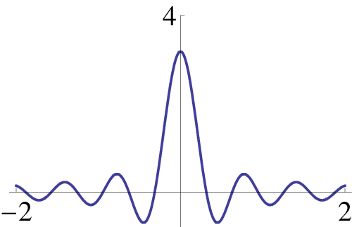
Define the Dirichlet kernel

Dn​(t)\displaystyle D_{n}(t) =∑j=−nnei​j​t\displaystyle=\sum_{j=-n}^{n}e^{ijt} (2.1)
=ei⁡(n+1)​t−e−i​n​tei​t−1\displaystyle=\frac{e^{i(n+1)t}-e^{-int}}{e^{it}-1} by geometric series (2.2)
=sin⁡((n+12)​t)sin⁡(12​t)\displaystyle=\frac{\sin\big((n+\frac{1}{2})t\big)}{\sin\big(\frac{1}{2}t\big)} (2.3)
Refer to caption
Figure 2.1: Dirichlet kernel with n=10n=10

(S1) holds by (2.1). You can show (optional exercise) that ∥Dn∥L1​(𝕋)∼(const.)​log⁡n\lVert D_{n}\rVert_{L^{1}({\mathbb{T}})}\sim(\text{const.})\log n as n→∞n\to\infty, so that (S2) fails.

∴{Dn}\therefore\ \{D_{n}\} is not a summability kernel.

Refer to caption
Figure 2.2: Fejér kernel with n=10n=10
Example 2.3.

Define the Fejér kernel

Fn​(t)\displaystyle F_{n}(t) =D0​(t)+⋯+Dn​(t)n+1\displaystyle=\frac{D_{0}(t)+\cdots+D_{n}(t)}{n+1} (2.4)
=∑j=−nn(1−|j|n+1)​ei​j​t\displaystyle=\sum_{j=-n}^{n}\left(1-\frac{|j|}{n+1}\right)e^{ijt} by (2.4) and (2.1) (2.5)
=1n+1​(sin⁡(n+12​t)sin⁡(12​t))2\displaystyle=\frac{1}{n+1}\left(\frac{\sin\big(\frac{n+1}{2}t\big)}{\sin\big(\frac{1}{2}t\big)}\right)^{\!\!\!2} by (2.4), (2.2) and geometric series (2.6)

(S1) holds by (2.5), and Fn≥0F_{n}\geq 0 so that (S2) holds also. For (S4),

supδ<|t|<π|Fn​(t)|\displaystyle\sup_{\delta<|t|<\pi}|F_{n}(t)| ≤1n+1​1sin2⁡(12​δ)\displaystyle\leq\frac{1}{n+1}\frac{1}{\sin^{2}\big(\frac{1}{2}\delta\big)} by (2.6)
→0\displaystyle\to 0 as n→∞n\to\infty.

∴{Fn}\therefore\ \{F_{n}\} is a positive summability kernel.

Example 2.4.

Define the Poisson kernel

Pr​(t)\displaystyle P_{r}(t) =1+2​∑j=1∞rj​cos⁡(j​t)\displaystyle=1+2\sum_{j=1}^{\infty}r^{j}\cos(jt) (2.7)
=∑j=−∞∞r|j|​ei​j​t\displaystyle=\sum_{j=-\infty}^{\infty}r^{|j|}e^{ijt} (2.8)
=1−r21−2​r​cos⁡t+r2\displaystyle=\frac{1-r^{2}}{1-2r\cos t+r^{2}} (2.9)

by summing two geometric series (j<0j<0 and j≥0j\geq 0) in (2.8) and simplifying.

The Poisson kernel is indexed by r∈(0,1)r\in(0,1), with limiting process r↗1r\nearrow 1. After suitably modifying the definition of summability kernel, we see (S1) holds by (2.7), and Pr≥0P_{r}\geq 0 by (2.9) so that (S2) holds also. For (S4),

supδ<|t|<π|Pr​(t)|\displaystyle\sup_{\delta<|t|<\pi}|P_{r}(t)| ≤1−r21−2​r​cos⁡δ+r2\displaystyle\leq\frac{1-r^{2}}{1-2r\cos\delta+r^{2}} by (2.9)
→0\displaystyle\to 0 as r↗1r\nearrow 1.

∴{Pr}\therefore\ \{P_{r}\} is a positive summability kernel.

Example 2.5.

Define the Gauss kernel

Gs​(t)\displaystyle G_{s}(t) =∑j=−∞∞e−j2​s​ei​j​t\displaystyle=\sum_{j=-\infty}^{\infty}e^{-j^{2}s}e^{ijt} (2.10)
=2​π4​π​s∑n=−∞∞e−(t+2πn)2/4s\displaystyle=\frac{2\pi}{\sqrt{4\pi s}}\sum_{n=-\infty}^{\infty}e^{-(t+2\pi n)^{2}/4s} (2.11)

by Example 23.7 later in the course.

Refer to caption
Figure 2.3: Poisson kernel with r=0.9r=0.9
Refer to caption
Figure 2.4: Gauss kernel with s=0.01s=0.01

The Gauss kernel is indexed by s∈(0,∞)s\in(0,\infty), with limiting process s↘0s\searrow 0. The analogue of (S1) holds by (2.10), and Gs≥0G_{s}\geq 0 by (2.11) so that (S2) holds also. For (S4),

supδ<|t|<π|Gs​(t)|\displaystyle\sup_{\delta<|t|<\pi}|G_{s}(t)| ≤2​π4​π​s[e−δ2/4s+∑n≠0e−(πn)2/4s]\displaystyle\leq\frac{2\pi}{\sqrt{4\pi s}}\left[e^{-\delta^{2}/4s}+\sum_{n\neq 0}e^{-(\pi n)^{2}/4s}\right] by (2.11)
→0\displaystyle\to 0 as s↘0s\searrow 0.

∴{Gs}\therefore\ \{G_{s}\} is a positive summability kernel.

Connection to Fourier series
Sn​(f)=Dn∗f\framebox{$S_{n}(f)=D_{n}*f$}

Proof. Dn​(t)​=(2.1)​∑j=−nn1​ei​j​tD_{n}(t)\overset{\eqref{eq:D1}}{=}\sum_{j=-n}^{n}1e^{ijt} implies

(Dn∗f)​(t)=∑j=−nn1​f^​(j)​ei​j​t=Sn​(f)(D_{n}*f)(t)=\sum_{j=-n}^{n}1\widehat{f}(j)e^{ijt}=S_{n}(f)

by Convolution Fact (1.4).

σn​(f)=Fn∗f\framebox{$\sigma_{n}(f)=F_{n}*f$}

Proof. Fn​(t)​=(2.4)​∑j=−nn(1−|j|n+1)​ei​j​tF_{n}(t)\overset{\eqref{eq:F1}}{=}\sum_{j=-n}^{n}(1-\frac{|j|}{n+1})e^{ijt} implies

(Fn∗f)​(t)=∑j=−nn(1−|j|n+1)​f^​(j)​ei​j​t=σn​(f)(F_{n}*f)(t)=\sum_{j=-n}^{n}\big(1-\frac{|j|}{n+1}\big)\widehat{f}(j)e^{ijt}=\sigma_{n}(f)

by Convolution Fact (1.4). Alternatively, use that σn​(f)=[S0​(f)+⋯+Sn​(f)]/(n+1)\sigma_{n}(f)=[S_{0}(f)+\cdots+S_{n}(f)]/(n+1) and Fn=[D0+⋯+Dn]/(n+1)F_{n}=[D_{0}+\cdots+D_{n}]/(n+1).

Thus for summability of Fourier series, we want Fn∗f→fF_{n}*f\to f.
Abel mean of S⁡[f]=Pr∗f\framebox{$\text{Abel mean of $S[f]$}=P_{r}*f$}

Proof. Pr​(t)​=(2.8)​∑j=−∞∞r|j|​ei​j​tP_{r}(t)\overset{\eqref{eq:P2}}{=}\sum_{j=-\infty}^{\infty}r^{|j|}e^{ijt} implies

(Pr∗f)​(t)=∑j=−∞∞r|j|​f^​(j)​ei​j​t(P_{r}*f)(t)=\sum_{j=-\infty}^{\infty}r^{|j|}\widehat{f}(j)e^{ijt} (2.12)

by Convolution Fact (1.4) (with the series converging absolutely and uniformly), and this last expression is the Abel mean of S⁡[f]S[f].

Summability in norm
Theorem 2.6 (Summability in Lp​(𝕋){L^{p}({\mathbb{T}})} and C⁡(𝕋)C({\mathbb{T}})).

If {kn}\{k_{n}\} is a summability kernel and f∈Lp​(𝕋),1≤p<∞f\in{L^{p}({\mathbb{T}})},1\leq p<\infty, then

kn∗f→fin Lp​(𝕋),  as n→∞.k_{n}*f\to f\qquad\text{in ${L^{p}({\mathbb{T}})}$, \hskip 10.22217ptas $n\to\infty$.}

Similarly, if f∈C⁡(𝕋)f\in C({\mathbb{T}}) then kn∗f→fk_{n}*f\to f in C⁡(𝕋)C({\mathbb{T}}).

Proof.

Let ε>0{\varepsilon}>0. By (S2) and continuity of translation on Lp​(𝕋){L^{p}({\mathbb{T}})} (Lemma 1.4), we can choose 0<δ<π0<\delta<\pi such that

max|τ|≤δ⁡∥fτ−f∥Lp​(𝕋)⋅supn∥kn∥L1​(𝕋)<ε.\max_{|\tau|\leq\delta}\lVert f_{\tau}-f\rVert_{L^{p}({\mathbb{T}})}\cdot\sup_{n}\lVert k_{n}\rVert_{L^{1}({\mathbb{T}})}<{\varepsilon}. (2.13)

Then

∥(kn∗f)​(t)−f⁡(t)∥Lp​(𝕋)\displaystyle\big\lVert(k_{n}*f)(t)-f(t)\big\rVert_{L^{p}({\mathbb{T}})}
=∥12​π​∫𝕋kn​(τ)​[fτ​(t)−f⁡(t)]​𝑑τ∥Lp​(𝕋)\displaystyle=\big\lVert\frac{1}{2\pi}\!\int_{\mathbb{T}}k_{n}(\tau)[f_{\tau}(t)-f(t)]\,d\tau\big\rVert_{L^{p}({\mathbb{T}})} by (S1)
≤12​π​∫𝕋|kn​(τ)|​∥fτ−f∥Lp​(𝕋)​𝑑τ\displaystyle\leq\frac{1}{2\pi}\!\int_{\mathbb{T}}|k_{n}(\tau)|\lVert f_{\tau}-f\rVert_{L^{p}({\mathbb{T}})}\,d\tau
      by Minkowski’s Integral Inequality, Theorem A.1,
=12​π(∫−δδ+∫{δ<|τ|<π})|kn(τ)|∥fτ−f∥Lp​(𝕋)dτ\displaystyle=\frac{1}{2\pi}\left(\int_{-\delta}^{\delta}+\int_{\{\delta<|\tau|<\pi\}}\right)|k_{n}(\tau)|\lVert f_{\tau}-f\rVert_{L^{p}({\mathbb{T}})}\,d\tau
≤max|τ|≤δ⁡∥fτ−f∥Lp​(𝕋)​12​π​∫−δδ|kn​(τ)|​𝑑τ\displaystyle\leq\max_{|\tau|\leq\delta}\lVert f_{\tau}-f\rVert_{L^{p}({\mathbb{T}})}\frac{1}{2\pi}\int_{-\delta}^{\delta}|k_{n}(\tau)|\,d\tau
+max|τ|≤π∥fτ−f∥Lp​(𝕋)12​π∫{δ<|τ|<π}|kn(τ)|dτ\displaystyle\quad+\max_{|\tau|\leq\pi}\lVert f_{\tau}-f\rVert_{L^{p}({\mathbb{T}})}\frac{1}{2\pi}\int_{\{\delta<|\tau|<\pi\}}|k_{n}(\tau)|\,d\tau
<ε+ε\displaystyle<{\varepsilon}+{\varepsilon}

by (2.13) and (S3), for all large nn.

If f∈C⁡(𝕋)f\in C({\mathbb{T}}) then repeat the argument with p=∞p=\infty, using uniform continuity of ff to get that fτ→ff_{\tau}\to f in L∞​(𝕋){L^{\infty}({\mathbb{T}})}. ∎

Consequences

∙\bullet Summability of Fourier series in C⁡(𝕋),Lp​(𝕋),1≤p<∞C({\mathbb{T}}),{L^{p}({\mathbb{T}})},1\leq p<\infty:

σn​(f)→f\sigma_{n}(f)\to f

in norm.

Proof. Choose kn=Fn=k_{n}=F_{n}= Fejér kernel. Then σn​(f)=Fn∗f→f\sigma_{n}(f)=F_{n}*f\to f in norm by Theorem 2.6.

∙\bullet Trigonometric polynomials are dense in C⁡(𝕋),Lp​(𝕋),1≤p<∞C({\mathbb{T}}),{L^{p}({\mathbb{T}})},1\leq p<\infty.

Proof. σn​(f)\sigma_{n}(f) is a trigonometric polynomial arbitrarily close to ff.

Aside. Density of trigonometric polynomials in C⁡(𝕋)C({\mathbb{T}}) proves the Weierstrass Trigonometric Approximation Theorem.

∙\bullet Uniqueness theorem:

if f,g∈L1​(𝕋)f,g\in{L^{1}({\mathbb{T}})} with f^​(n)=g^​(n)\widehat{f}(n)=\widehat{g}(n) for all nn, then f=gf=g in L1​(𝕋){L^{1}({\mathbb{T}})}. (2.14)

In other words, the map ^:L1​(𝕋)→ℓ∞​(ℤ)\widehat{\ }:{L^{1}({\mathbb{T}})}\to\ell^{\infty}({\mathbb{Z}}) is injective.

Proof. Fn∗f=Fn∗gF_{n}*f=F_{n}*g by Convolution Fact (1.4), since f^=g^\widehat{f}=\widehat{g}. Letting n→∞n\to\infty gives f=gf=g.

Connection to PDEs

To finish the section, we connect our summability kernels to some important partial differential equations. Fix f∈L1​(𝕋)f\in{L^{1}({\mathbb{T}})}.

1. The Poisson kernel solves Laplace’s equation in a disk:

v⁡(r​ei​t)=(Pr∗f)​(t)=12​π​∫𝕋1−r21−2​r​cos⁡(t−τ)+r2​f​(τ)​𝑑τv(re^{it})=(P_{r}*f)(t)=\frac{1}{2\pi}\int_{\mathbb{T}}\frac{1-r^{2}}{1-2r\cos(t-\tau)+r^{2}}f(\tau)\,d\tau

solves

Δ​v=vr​r+r−1​vr+r−2​vt​t=0\Delta v=v_{rr}+r^{-1}v_{r}+r^{-2}v_{tt}=0

on the unit disk {r<1}\{r<1\}, with boundary value v⁡(1,t)=f⁡(t)v(1,t)=f(t) in the sense of Theorem 2.6.

That is, vv is the harmonic extension of ff from the boundary circle to the disk.

Proof. Differentiate through formula (2.12) for Pr∗fP_{r}*f and note that

(∂2∂r2+1r​∂∂r+1r2​∂2∂t2)​(r|j|​ei​j​t)=0.\Big(\frac{\partial^{2}\ }{\partial r^{2}}+\frac{1}{r}\frac{\partial\ }{\partial r}+\frac{1}{r^{2}}\frac{\partial^{2}\ }{\partial t^{2}}\Big)(r^{|j|}e^{ijt})=0.

2. The Gauss kernel solves the diffusion (heat) equation:

w⁡(s,t)=(Gs∗f)​(t)w(s,t)=(G_{s}*f)(t)

solves

ws=wt​tw_{s}=w_{tt}

for (s,t)∈(0,∞)×𝕋(s,t)\in(0,\infty)\times{\mathbb{T}}, with initial value w⁡(0,t)=f⁡(t)w(0,t)=f(t) in the sense of Theorem 2.6.

Proof. Gs​(t)​=(2.10)​∑j=−∞∞e−j2​s​ei​j​tG_{s}(t)\overset{\eqref{eq:G1}}{=}\sum_{j=-\infty}^{\infty}e^{-j^{2}s}e^{ijt} implies

(Gs∗f)​(t)=∑j=−∞∞e−j2​s​f^​(j)​ei​j​t(G_{s}*f)(t)=\sum_{j=-\infty}^{\infty}e^{-j^{2}s}\widehat{f}(j)e^{ijt}

by Convolution Fact (1.4). Now differentiate through the sum and use that

(∂∂s−∂2∂t2)​(e−j2​s​ei​j​t)=0.\left(\frac{\partial\ }{\partial s}-\frac{\partial^{2}\ }{\partial t^{2}}\right)(e^{-j^{2}s}e^{ijt})=0.

Chapter 3 Fourier series: summability at a point

Goal

Prove a sufficient condition for summability at a point

Reference

[Katznelson] Section I.3

By Chapter 2, if ff is continuous then σn​(f)→f\sigma_{n}(f)\to f in C⁡(𝕋)C({\mathbb{T}}). That is, σn​(f)→f\sigma_{n}(f)\to f uniformly. In particular, σn​(f)​(t)→f⁡(t)\sigma_{n}(f)(t)\to f(t), for each t∈𝕋t\in{\mathbb{T}}.

But what if ff is merely continuous at a point?

Theorem 3.1 (Summability at a point).

Assume {kn}\{k_{n}\} is a summability kernel,f∈L1​(𝕋)f\in{L^{1}({\mathbb{T}})} and t0∈𝕋t_{0}\in{\mathbb{T}}. Suppose either {kn}\{k_{n}\} satisfies the L∞L^{\infty} concentration hypothesis (S4), or else f∈L∞​(𝕋)f\in{L^{\infty}({\mathbb{T}})}.

(a) If ff is continuous at t0t_{0} then (kn∗f)​(t0)→f⁡(t0)(k_{n}*f)(t_{0})\to f(t_{0}) as n→∞n\to\infty.

(b) If in addition the summability kernel is even (kn​(−t)=kn​(t)k_{n}(-t)=k_{n}(t)) and

L=limh→0f⁡(t0+h)+f⁡(t0−h)2L=\lim_{h\to 0}\frac{f(t_{0}+h)+f(t_{0}-h)}{2}

exists (or equals ±∞\pm\infty), then

(kn∗f)​(t0)→Las n→∞.(k_{n}*f)(t_{0})\to L\qquad\text{as $n\to\infty$.}

Note if ff has limits from the left and right at t0t_{0}, then the quantity LL equals the average of those limits.

The Fejér and Poisson kernels satisfy (SR4), and so Theorem 3.1 applies in particular to summability at a point for σn​(f)=Fn∗f\sigma_{n}(f)=F_{n}*f and for the Abel mean Pr∗fP_{r}*f.

Proof.

(a) Let ε>0{\varepsilon}>0 and choose 0<δ<π0<\delta<\pi such that

supn∥kn∥L1​(𝕋)⋅max|τ|≤δ⁡|f⁡(t0−τ)−f⁡(t0)|<ε,\sup_{n}\lVert k_{n}\rVert_{L^{1}({\mathbb{T}})}\cdot\max_{|\tau|\leq\delta}|f(t_{0}-\tau)-f(t_{0})|<{\varepsilon}, (3.1)

using here (S2) and continuity of ff at t0t_{0}. Then as n→∞n\to\infty,

|(kn∗f)​(t0)−f⁡(t0)|\displaystyle|(k_{n}*f)(t_{0})-f(t_{0})|
=|∫{|τ|<δ}kn(τ)[f(t0−τ)−f(t0)]dτ\displaystyle=\Big|\int_{\{|\tau|<\delta\}}k_{n}(\tau)[f(t_{0}-\tau)-f(t_{0})]\,d\tau
−∫{δ<|τ|<π}kn(τ)dτ⋅f(t0)+∫{δ<|τ|<π}kn(τ)f(t0−τ)dτ|using (S1)\displaystyle\qquad-\int_{\{\delta<|\tau|<\pi\}}k_{n}(\tau)\,d\tau\cdot f(t_{0})+\int_{\{\delta<|\tau|<\pi\}}k_{n}(\tau)f(t_{0}-\tau)\,d\tau\Big|\qquad\text{using \eqref{eq:S1}}
<{ε+o⁡(1)+o⁡(1)⋅∥f∥L1​(𝕋)by (3.1), (S3) and (S4), or elseε+o⁡(1)+o⁡(1)⋅∥f∥L∞​(𝕋)by (3.1), (S3) and (S1),\displaystyle<\begin{cases}{\varepsilon}+o(1)+o(1)\cdot\lVert f\rVert_{L^{1}({\mathbb{T}})}&\text{by \eqref{eq:sp1}, \eqref{eq:S3} and \eqref{eq:S4}, or else}\\ {\varepsilon}+o(1)+o(1)\cdot\lVert f\rVert_{L^{\infty}({\mathbb{T}})}&\text{by \eqref{eq:sp1}, \eqref{eq:S3} and \eqref{eq:S1},}\end{cases}
<ε\displaystyle<{\varepsilon}

for all large nn.

(b) The proof is similar to (a), but uses symmetry of the kernel. ∎

Remark 3.2.

1. How does the proof of summability at a point, in Theorem 3.1(a), differ from the proof of summability in norm, in Theorem 2.6?

2. Theorem 3.1 treats summability at a single point t0t_{0} at which ff is continuous. Chapter 7 will prove kn∗f→fk_{n}*f\to f at almost every point, for each integrable ff.

Chapter 4 Fourier coefficients in ℓ1​(ℤ)\ell^{1}({\mathbb{Z}}) (or, f∈A⁡(𝕋)f\in A({\mathbb{T}}))

Goal

Establish the algebra structure of A⁡(𝕋)A({\mathbb{T}})

Reference

[Katznelson] Section I.6

Define

A⁡(𝕋)\displaystyle A({\mathbb{T}}) ={f∈L1​(𝕋):∑n∈ℤ|f^​(n)|<∞}\displaystyle=\{f\in{L^{1}({\mathbb{T}})}:\sum_{n\in{\mathbb{Z}}}|\widehat{f}(n)|<\infty\}
=functions with Fourier coefficients in ℓ1​(ℤ).\displaystyle=\text{functions with Fourier coefficients in $\ell^{1}({\mathbb{Z}})$.}

The map ^:A⁡(𝕋)→ℓ1​(ℤ)\widehat{\ }:A({\mathbb{T}})\to\ell^{1}({\mathbb{Z}}) is a linear bijection.

Proof. Injectivity follows from the uniqueness result (2.14). To prove surjectivity, let {cn}∈ℓ1​(ℤ)\{c_{n}\}\in\ell^{1}({\mathbb{Z}}) and define g⁡(t)=∑n∈ℤcn​ei​n​tg(t)=\sum_{n\in{\mathbb{Z}}}c_{n}e^{int}. The series for gg converges uniformly since

supt∈𝕋|∑|n|>Ncn​ei​n​t|≤∑|n|>N|cn|→0\sup_{t\in{\mathbb{T}}}\big|\sum_{|n|>N}c_{n}e^{int}\big|\leq\sum_{|n|>N}|c_{n}|\to 0

as N→∞N\to\infty. (Hence gg is continuous.) We have g^​(m)=cm\widehat{g}(m)=c_{m} for every mm, and so g^={cm}\widehat{g}=\{c_{m}\} as desired.

Our proof has shown each f∈A⁡(𝕋)f\in A({\mathbb{T}}) is represented by its Fourier series:

f⁡(t)=∑n∈ℤf^​(n)​ei​n​ta.e.f(t)=\sum_{n\in{\mathbb{Z}}}\widehat{f}(n)e^{int}\quad\text{a.e.} (4.1)

so that ff is continuous (after redefinition on a set of measure zero). This Fourier series converges absolutely and uniformly.

Definition 4.1.

Define a norm on A⁡(𝕋)A({\mathbb{T}}) by

∥f∥A⁡(𝕋)=∥f^∥ℓ1​(ℤ)=∑n|f^​(n)|.\lVert f\rVert_{A({\mathbb{T}})}=\lVert\widehat{f}\rVert_{\ell^{1}({\mathbb{Z}})}=\sum_{n}|\widehat{f}(n)|.

A⁡(𝕋)A({\mathbb{T}}) is a Banach space under this norm (because ℓ1​(ℤ)\ell^{1}({\mathbb{Z}}) is one).

Define the convolution of sequences a,b∈ℓ1​(ℤ)a,b\in\ell^{1}({\mathbb{Z}}) by

(a∗b)​(n)=∑m∈ℤa⁡(m)​b​(n−m).(a*b)(n)=\sum_{m\in{\mathbb{Z}}}a(m)b(n-m).

Clearly

∥a∗b∥ℓ1​(ℤ)≤∥a∥ℓ1​(ℤ)​∥b∥ℓ1​(ℤ)\lVert a*b\rVert_{\ell^{1}({\mathbb{Z}})}\leq\lVert a\rVert_{\ell^{1}({\mathbb{Z}})}\lVert b\rVert_{\ell^{1}({\mathbb{Z}})} (4.2)

because

∑n|(a∗b)​(n)|≤∑m|a⁡(m)|​∑n|b⁡(n−m)|=∥a∥ℓ1​(ℤ)​∥b∥ℓ1​(ℤ).\sum_{n}|(a*b)(n)|\leq\sum_{m}|a(m)|\sum_{n}|b(n-m)|=\lVert a\rVert_{\ell^{1}({\mathbb{Z}})}\lVert b\rVert_{\ell^{1}({\mathbb{Z}})}.
Theorem 4.2 ( ^\widehat{\ } takes multiplication to convolution).

A⁡(𝕋)A({\mathbb{T}}) is an algebra, meaning that if f,g∈A⁡(𝕋)f,g\in A({\mathbb{T}}) then f​g∈A⁡(𝕋)fg\in A({\mathbb{T}}). Indeed

f​g^=f^∗g^\widehat{fg}=\widehat{f}*\widehat{g}

and ∥f​g∥A⁡(𝕋)≤∥f∥A⁡(𝕋)​∥g∥A⁡(𝕋)\lVert fg\rVert_{A({\mathbb{T}})}\leq\lVert f\rVert_{A({\mathbb{T}})}\lVert g\rVert_{A({\mathbb{T}})}.

Proof.

f​gfg is continuous, and hence integrable, with

(f​g)^​(n)\displaystyle\widehat{(fg)}(n) =12​π​∫𝕋f⁡(t)​g​(t)​e−i​n​t​𝑑t\displaystyle=\frac{1}{2\pi}\!\int_{{\mathbb{T}}}f(t)g(t)e^{-int}dt
=∑mf^​(m)​12​π​∫𝕋g⁡(t)​e−i⁡(n−m)​t​𝑑t\displaystyle=\sum_{m}\widehat{f}(m)\frac{1}{2\pi}\!\int_{{\mathbb{T}}}g(t)e^{-i(n-m)t}\,dt by (4.1)
=∑mf^​(m)​g^​(n−m)\displaystyle=\sum_{m}\widehat{f}(m)\widehat{g}(n-m)
=(f^∗g^)​(n).\displaystyle=(\widehat{f}*\widehat{g})(n).

So ∥(f​g)^∥ℓ1​(ℤ)≤∥f^∥ℓ1​(ℤ)​∥g^∥ℓ1​(ℤ)\lVert\widehat{(fg)}\rVert_{\ell^{1}({\mathbb{Z}})}\leq\lVert\widehat{f}\rVert_{\ell^{1}({\mathbb{Z}})}\lVert\widehat{g}\rVert_{\ell^{1}({\mathbb{Z}})} by (4.2). ∎

Sufficient conditions for membership in A⁡(𝕋)A({\mathbb{T}}) are discussed in [Katznelson, Section I.6], for example, Hölder continuity: Cα​(𝕋)⊂A​(𝕋)C^{\alpha}({\mathbb{T}})\subset A({\mathbb{T}}) when α>12\alpha>\frac{1}{2}.

Theorem 4.3 (Wiener’s Inversion Theorem).

If f∈A⁡(𝕋)f\in A({\mathbb{T}}) and f⁡(t)≠0f(t)\neq 0 for every t∈𝕋t\in{\mathbb{T}} then 1/f∈A⁡(𝕋)1/f\in A({\mathbb{T}}).

We omit the proof. Clearly 1/f1/f is continuous, but it is not clear that (1/f)^\widehat{(1/f)} belongs to ℓ1​(ℤ)\ell^{1}({\mathbb{Z}}).

Chapter 5 Fourier coefficients in ℓ2​(ℤ)\ell^{2}({\mathbb{Z}}) (or, f∈L2​(𝕋)f\in{L^{2}({\mathbb{T}})})

Goal

Study the Fourier ONB for L2​(𝕋){L^{2}({\mathbb{T}})}, using analysis and synthesis operators

Notation and definitions

Let HH be a Hilbert space with inner product ⟨u,v⟩\langle u,v\rangle and norm ∥u∥=⟨u,u⟩\lVert u\rVert=\sqrt{\langle u,u\rangle}.

Given a sequence {un}n∈ℤ\{u_{n}\}_{n\in{\mathbb{Z}}} in HH, define the

synthesis operator ​S:ℓ2​(ℤ)\displaystyle\textbf{synthesis operator\hskip 11.49994pt}S:\ell^{2}({\mathbb{Z}}) →H\displaystyle\to H
{cn}n∈ℤ\displaystyle\{c_{n}\}_{n\in{\mathbb{Z}}} ↦∑ncn​un\displaystyle\mapsto\sum_{n}c_{n}u_{n}

and

analysis operator ​T:H\displaystyle\textbf{analysis operator\hskip 11.49994pt}T:H →ℓ2​(ℤ)\displaystyle\to\ell^{2}({\mathbb{Z}})
u\displaystyle u ↦{⟨u,un⟩}n∈ℤ.\displaystyle\mapsto\{\langle u,u_{n}\rangle\}_{n\in{\mathbb{Z}}}.
Theorem 5.1.

If analysis is bounded (∑n|⟨u,un⟩|2≤(const.)​∥u∥2\sum_{n}|\langle u,u_{n}\rangle|^{2}\leq(\text{const.})\lVert u\rVert^{2} for all u∈Hu\in H), then so is synthesis, and the series S⁡({cn})=∑cn​unS(\{c_{n}\})=\sum c_{n}u_{n} converges unconditionally.

Proof.

Since TT is bounded, the adjoint T∗:ℓ2​(ℤ)→HT^{*}:\ell^{2}({\mathbb{Z}})\to H is bounded, and for each sequence {cn},u∈H,N≥1\{c_{n}\},u\in H,N\geq 1, we have

⟨T∗​({cn}n=−NN),u⟩\displaystyle\langle T^{*}(\{c_{n}\}_{n=-N}^{N}),u\rangle =⟨{cn}n=−NN,T​u⟩ℓ2\displaystyle=\langle\{c_{n}\}_{n=-N}^{N},Tu\rangle_{\ell^{2}}
=∑n=−NNcn⟨u,un⟩¯by definition of T​u\displaystyle=\sum_{n=-N}^{N}c_{n}\overline{\langle u,u_{n}\rangle}\qquad\text{by definition of $Tu$}
=⟨∑n=−NNcn​un,u⟩.\displaystyle=\langle\sum_{n=-N}^{N}c_{n}u_{n},u\rangle.

Hence T∗​({cn}n=−NN)=∑n=−NNcn​unT^{*}(\{c_{n}\}_{n=-N}^{N})=\sum_{n=-N}^{N}c_{n}u_{n}. The limit as N→∞N\to\infty exists on the left side, and hence on the right side; therefore T∗​({cn})=∑n=−∞∞cn​unT^{*}(\{c_{n}\})=\sum_{n=-\infty}^{\infty}c_{n}u_{n}, so that T∗=ST^{*}=S. Hence SS is bounded.

Convergence of the synthesis series is unconditional, because if A⊂ℤA\subset{\mathbb{Z}} then

∥S⁡({cn}n∈ℤ)−S⁡({cn}n∈A)∥\displaystyle\big\lVert S(\{c_{n}\}_{n\in{\mathbb{Z}}})-S(\{c_{n}\}_{n\in A})\big\rVert =∥S⁡({cn}n∈ℤ∖A)∥\displaystyle=\big\lVert S(\{c_{n}\}_{n\in{\mathbb{Z}}\setminus A})\big\rVert
≤∥S∥​∥{cn}∥ℓ2​(ℤ∖A),\displaystyle\leq\lVert S\rVert\lVert\{c_{n}\}\rVert_{\ell^{2}({\mathbb{Z}}\setminus A)},

which tends to 00 as AA expands to fill ℤ{\mathbb{Z}}, regardless of the order in which AA expands. ∎

Remark 5.2.

The last proof shows S=T∗S=T^{*}, meaning

analysis and synthesis are adjoint operations.
Theorem 5.3 (Fourier coefficients on L2​(𝕋){L^{2}({\mathbb{T}})}).

The Fourier coefficient (or analysis) operator ^:L2​(𝕋)→ℓ2​(ℤ)\widehat{\ }:{L^{2}({\mathbb{T}})}\to\ell^{2}({\mathbb{Z}}) is an isometry, with

∥f∥L2​(𝕋)\displaystyle\lVert f\rVert_{L^{2}({\mathbb{T}})} =∥f^∥ℓ2​(ℤ)\displaystyle=\lVert\widehat{f}\rVert_{\ell^{2}({\mathbb{Z}})} (Plancherel)
⟨f,g⟩L2​(𝕋)\displaystyle\langle f,g\rangle_{{L^{2}({\mathbb{T}})}} =⟨f^,g^⟩ℓ2​(ℤ)\displaystyle=\langle\widehat{f},\widehat{g}\rangle_{\ell^{2}({\mathbb{Z}})} (Parseval)

for all f,g∈L2​(𝕋)f,g\in{L^{2}({\mathbb{T}})}.

Proof.

First we prove Plancherel’s identity: since Pr∗f→fP_{r}*f\to f in L2​(𝕋){L^{2}({\mathbb{T}})} by Theorem 2.6, we have

12​π​∫𝕋|f⁡(t)|2​𝑑t\displaystyle\frac{1}{2\pi}\!\int_{\mathbb{T}}|f(t)|^{2}\,dt =limr→112​π​∫𝕋f⁡(t)​(Pr∗f)​(t)¯​𝑑t\displaystyle=\lim_{r\to 1}\frac{1}{2\pi}\!\int_{\mathbb{T}}f(t)\overline{(P_{r}*f)(t)}\,dt
=limr→112​π∫𝕋f(t)∑n∈ℤr|n|​f^​(n)​ei​n​t¯dtby (2.12) for Pr∗f\displaystyle=\lim_{r\to 1}\frac{1}{2\pi}\!\int_{\mathbb{T}}f(t)\sum_{n\in{\mathbb{Z}}}\overline{r^{|n|}\widehat{f}(n)e^{int}}\,dt\qquad\text{by \eqref{eq:pabel} for $P_{r}*f$}
=limr→1∑n∈ℤr|n|​|f^​(n)|2\displaystyle=\lim_{r\to 1}\sum_{n\in{\mathbb{Z}}}r^{|n|}|\widehat{f}(n)|^{2}
=∑n∈ℤ|f^​(n)|2\displaystyle=\sum_{n\in{\mathbb{Z}}}|\widehat{f}(n)|^{2}

by monotone convergence.

Parseval follows from Plancherel by polarization, or by repeating the argument for Plancherel with ⟨f,f⟩\langle f,f\rangle changed to ⟨f,g⟩\langle f,g\rangle (and using dominated instead of monotone convergence). ∎

Since the Fourier analysis operator is bounded, so is its adjoint, the Fourier synthesis operator

ˇ:ℓ2​(ℤ)\displaystyle\check{\ }:\ell^{2}({\mathbb{Z}}) →L2​(𝕋)\displaystyle\to{L^{2}({\mathbb{T}})}
{cn}n∈ℤ\displaystyle\{c_{n}\}_{n\in{\mathbb{Z}}} ↦∑ncn​ei​n​t\displaystyle\mapsto\sum_{n}c_{n}e^{int}
Theorem 5.4 (Fourier ONB).

(a) If f∈L2​(𝕋)f\in{L^{2}({\mathbb{T}})} then ∑nf^​(n)​ei​n​t=f\sum_{n}\widehat{f}(n)e^{int}=f with unconditional convergence in L2​(𝕋){L^{2}({\mathbb{T}})}. That is, (f^)​ˇ=f(\hat{f})\check{\ }=f.

(b) If c={cn}∈ℓ2​(ℤ)c=\{c_{n}\}\in\ell^{2}({\mathbb{Z}}) then (∑n∈ℤcn​ei​n​t)​^​(j)=cj(\ \sum_{n\in{\mathbb{Z}}}c_{n}e^{int})\widehat{\ }(j)=c_{j}. That is, (cˇ)​^=c(\check{c})\hat{\ }=c.

(c) {ei​n​t}n∈ℤ\{e^{int}\}_{n\in{\mathbb{Z}}} is an orthonormal basis of L2​(𝕋){L^{2}({\mathbb{T}})}.

Part (a) says Fourier series converge in L2​(𝕋){L^{2}({\mathbb{T}})}. Parts (a) and (b) together show that Fourier analysis and synthesis are inverse operations.

Proof.

Fourier analysis and synthesis are bounded operators, and analysis followed by synthesis equals the identity (∑nf^​(n)​ei​n​t=f\sum_{n}\widehat{f}(n)e^{int}=f) on the class of trigonometric polynomials. That class is dense in L2​(𝕋){L^{2}({\mathbb{T}})}, and so by continuity, analysis followed by synthesis equals the identity on L2​(𝕋){L^{2}({\mathbb{T}})}.

Argue similarly for part (b), using the dense class of finite sequences in ℓ2​(ℤ)\ell^{2}({\mathbb{Z}}).

For orthonormality in part (c), observe

⟨ei​n​t,ei​m​t⟩=12​π​∫𝕋ei​n​t​e−i​m​t​𝑑t={1if n=m,0if n≠m.\langle e^{int},e^{imt}\rangle=\frac{1}{2\pi}\!\int_{\mathbb{T}}e^{int}e^{-imt}\,dt\\ =\begin{cases}1&\text{if $n=m$,}\\ 0&\text{if $n\neq m$.}\end{cases}

The basis property follows from part (a), noting f^​(n)=⟨f,ei​n​t⟩L2​(𝕋)\widehat{f}(n)=\langle f,e^{int}\rangle_{L^{2}({\mathbb{T}})}. ∎

Remark 5.5.

Fourier analysis satisfies

^\displaystyle\widehat{\ } :L1​(𝕋)→ℓ∞​(ℤ)\displaystyle:{L^{1}({\mathbb{T}})}\to\ell^{\infty}({\mathbb{Z}}) by Theorem 1.2,
^\displaystyle\widehat{\ } :L2​(𝕋)→ℓ2​(ℤ)\displaystyle:{L^{2}({\mathbb{T}})}\to\ell^{2}({\mathbb{Z}}) (isometrically) by Theorem 5.3.

Further, ^:L2​(𝕋)→ℓ2​(ℤ)\widehat{\ }:{L^{2}({\mathbb{T}})}\to\ell^{2}({\mathbb{Z}}) is a linear bijection by Theorem 5.4.

In Chapter 13 we will interpolate to show

^:Lp​(𝕋)→ℓp′​(ℤ),whenever ​1≤p≤2,1p+1p′=1.\widehat{\ }:{L^{p}({\mathbb{T}})}\to\ell^{p^{\prime}}({\mathbb{Z}}),\qquad\text{whenever\ }1\leq p\leq 2,\quad\frac{1}{p}+\frac{1}{p^{\prime}}=1.

Chapter 6 Maximal functions

Goals

Connect abstract maximal functions to convergence a.e.

Prove weak and strong bounds on the Hardy–Littlewood maximal function

Prepare for summability pointwise a.e. in next Chapter

References

[Duoandikoetxea] Section 2.2

[Grafakos] Section 2.1

[Stein] Section 1.1

Definition 6.1 (Weak and strong operators).

Let (X,μ)(X,\mu) and (Y,ν)(Y,\nu) be measure spaces, and 1≤p,q≤∞1\leq p,q\leq\infty. Suppose

T:Lp​(X)→{measurable functions on Y}.T:{L^{p}}(X)\to\{\text{measurable functions on $Y$}\}.

(We do not assume TT is linear.)

Call TT strong (𝐩,𝐪)\mathbf{(p,q)} if TT is bounded from Lp​(X){L^{p}}(X) to Lq​(Y)L^{q}(Y), meaning a constant C>0C>0 exists such that

∥T​f∥Lq​(Y)≤C​∥f∥Lp​(X),f∈Lp​(X).\lVert Tf\rVert_{L^{q}(Y)}\leq C\lVert f\rVert_{{L^{p}}(X)},\qquad f\in{L^{p}}(X).

When q<∞q<\infty, we call TT weak (𝐩,𝐪)\mathbf{(p,q)} if C>0C>0 exists such that

ν​({y∈Y:|(T​f)​(y)|>λ})1/q≤C​∥f∥Lp​(X)λ∀λ>0,f∈Lp​(X).\nu\big(\{y\in Y:|(Tf)(y)|>\lambda\}\big)^{1/q}\leq\frac{C\lVert f\rVert_{{L^{p}}(X)}}{\lambda}\qquad\forall\ \lambda>0,\quad f\in{L^{p}}(X).

When q=∞q=\infty, we call TT weak (𝐩,∞)\mathbf{(p,\infty)} if it is strong (p,∞)(p,\infty):

∥T​f∥L∞​(Y)≤C​∥f∥Lp​(X),f∈Lp​(X).\lVert Tf\rVert_{L^{\infty}(Y)}\leq C\lVert f\rVert_{{L^{p}}(X)},\qquad f\in{L^{p}}(X).
Lemma 6.2.

Strong (p,q)(p,q) ⇒\Rightarrow weak (p,q)(p,q).

Proof.

When q=∞q=\infty the result is immediate by definition. Suppose q<∞q<\infty. Write

E⁡(λ)={y∈Y:|(T​f)​(y)|>λ}E(\lambda)=\{y\in Y:|(Tf)(y)|>\lambda\}

for the level set of T​fTf above height λ\lambda. Then

λq​ν​(E⁡(λ))\displaystyle\lambda^{q}\,\nu\big(E(\lambda)\big) =∫E⁡(λ)λq​𝑑ν​(y)\displaystyle=\int_{E(\lambda)}\lambda^{q}\,d\nu(y)
≤∫E⁡(λ)|(T​f)​(y)|q​𝑑ν​(y)\displaystyle\leq\int_{E(\lambda)}|(Tf)(y)|^{q}\,d\nu(y) since λ<|T​f|\lambda<|Tf| on E⁡(λ)E(\lambda)
≤∥T​f∥Lq​(Y)q\displaystyle\leq\lVert Tf\rVert^{q}_{L^{q}(Y)}

and so

ν​(E⁡(λ))1/q\displaystyle\nu\big(E(\lambda)\big)^{1/q} ≤∥T​f∥Lq​(Y)λ\displaystyle\leq\frac{\lVert Tf\rVert_{L^{q}(Y)}}{\lambda}
≤C​∥f∥Lp​(X)λ\displaystyle\leq\frac{C\lVert f\rVert_{{L^{p}}(X)}}{\lambda}

if T is strong (p,q)(p,q). ∎

Lemma 6.3.

If TT is weak (p,q)(p,q) then T​f∈Ll​o​cr​(Y)Tf\in L^{r}_{loc}(Y) for all 0<r<q0<r<q.

Thus intuitively, TT “almost” maps LpL^{p} into LqL^{q}, locally.

Proof.

Let f∈Lp​(X)f\in{L^{p}}(X) and suppose Z⊂YZ\subset Y with ν⁡(Z)<∞\nu(Z)<\infty. We will show T​f∈Lr​(Z)Tf\in L^{r}(Z).

Write g=T​fg=Tf. Then

∫Z|g⁡(y)|r​𝑑ν​(y)\displaystyle\int_{Z}|g(y)|^{r}\,d\nu(y)
=∫0∞r​λr−1​ν​({y∈Z:|g⁡(y)|>λ})​𝑑λ\displaystyle=\int_{0}^{\infty}r\lambda^{r-1}\nu\big(\{y\in Z:|g(y)|>\lambda\}\big)\,d\lambda by AppendixB
≤∫01r​λr−1​ν​(Z)​𝑑λ+∫1∞r​λr−1​(C​∥f∥Lp​(X)λ)q​𝑑λ\displaystyle\leq\int_{0}^{1}r\lambda^{r-1}\nu(Z)\,d\lambda+\int_{1}^{\infty}r\lambda^{r-1}\Big(\frac{C\lVert f\rVert_{{L^{p}}(X)}}{\lambda}\Big)^{\!\!q}\,d\lambda by weak (p,q)(p,q)
<∞\displaystyle<\infty

since ν⁡(Z)<∞\nu(Z)<\infty and ∫1∞λ−1−q+r​𝑑λ<∞\int_{1}^{\infty}\lambda^{-1-q+r}\,d\lambda<\infty (using that −q+r<0-q+r<0). ∎

Theorem 6.4 (Maximal functions and convergence a.e.).

Assume

Tn:Lp​(X)→{measurable functions on X}T_{n}:L^{p}(X)\to\{\text{measurable functions on $X$}\}

for n=1,2,3,…n=1,2,3,\ldots. Define

T∗:Lp​(X)→{measurable functions on X}T^{*}:L^{p}(X)\to\{\text{measurable functions on $X$}\}

by

(T∗​f)​(x)=supn|(Tn​f)​(x)|,x∈X.(T^{*}f)(x)=\sup_{n}|(T_{n}f)(x)|,\qquad x\in X.

If T∗T^{*} is weak (p,q)(p,q) and each TnT_{n} is linear, then the collection

𝒞={f∈Lp​(X):limn(Tn​f)​(x)=f⁡(x)​a.e}{\mathcal{C}}=\{f\in L^{p}(X):\lim_{n}(T_{n}f)(x)=f(x)\ \text{a.e}\}

is closed in Lp​(X)L^{p}(X).

T∗T^{*} is called the maximal operator for the family {Tn}\{T_{n}\}. Clearly it takes values in [0,∞][0,\infty]. Note T∗T^{*} is not linear, in general.

Remark 6.5.

In this theorem a quantitative hypothesis (weak (p,q)(p,q)) implies a qualitative conclusion (closure of the collection 𝒞\mathcal{C} where Tn​f→fT_{n}f\to f a.e.).

Proof.

Let fk∈𝒞f_{k}\in{\mathcal{C}} with fk→ff_{k}\to f in Lp​(X)L^{p}(X). We show f∈𝒞f\in{\mathcal{C}}.

Suppose q<∞q<\infty. For any λ>0\lambda>0,

μ({x∈X:lim supn|(Tnf(x)−f(x)|>2λ})\displaystyle\mu\big(\{x\in X:\limsup_{n}|(T_{n}f(x)-f(x)|>2\lambda\}\big)
=μ⁡({x∈X:lim supn|Tn​(f−fk)​(x)−(f−fk)​(x)|>2​λ})\displaystyle=\mu\big(\{x\in X:\limsup_{n}|T_{n}(f-f_{k})(x)-(f-f_{k})(x)|>2\lambda\}\big)
    by linearity and the pointwise convergence Tn​fk→fkT_{n}f_{k}\to f_{k} a.e.
≤μ({x∈X:T∗(f−fk)(x)+|(f−fk)(x)|>2λ})by triangle inequality\displaystyle\leq\mu\big(\{x\in X:T^{*}(f-f_{k})(x)+|(f-f_{k})(x)|>2\lambda\}\big)\qquad\text{by triangle inequality}
≤μ⁡({x∈X:T∗​(f−fk)​(x)>λ})+μ⁡({x∈X:|(f−fk)​(x)|>λ})\displaystyle\leq\mu\big(\{x\in X:T^{*}(f-f_{k})(x)>\lambda\}\big)+\mu\big(\{x\in X:|(f-f_{k})(x)|>\lambda\}\big)
≤(C​∥f−fk∥Lp​(X)λ)q+(∥f−fk∥Lp​(X)λ)pby weak (p,q) on T∗\displaystyle\leq\Big(\frac{C\lVert f-f_{k}\rVert_{L^{p}(X)}}{\lambda}\Big)^{\!q}+\Big(\frac{\lVert f-f_{k}\rVert_{L^{p}(X)}}{\lambda}\Big)^{\!p}\qquad\text{by weak $(p,q)$ on $T^{*}$}
→0\displaystyle\to 0

as k→∞k\to\infty.

Therefore lim supn|(Tn​f)​(x)−f⁡(x)|≤2​λ\limsup_{n}|(T_{n}f)(x)-f(x)|\leq 2\lambda a.e. Taking a countable sequence of λ↘0\lambda\searrow 0, we conclude lim supn|(Tn​f)​(x)−f⁡(x)|=0\limsup_{n}|(T_{n}f)(x)-f(x)|=0 a.e. Therefore limn(Tn​f)​(x)=f⁡(x)\lim_{n}(T_{n}f)(x)=f(x) a.e., so that f∈𝒞f\in{\mathcal{C}}.

The case q=∞q=\infty is left to the reader. ∎

To apply maximal functions on ℝd{{\mathbb{R}}^{d}} and 𝕋{\mathbb{T}}, we will need:

Lemma 6.6 (Covering).

Let {Bi}i=1k\{B_{i}\}_{i=1}^{k} be a finite collection of open balls in ℝd{{\mathbb{R}}^{d}}. Then there exists a pairwise disjoint subcollection {Bij}j=1l\{B_{i_{j}}\}_{j=1}^{l} of balls such that

|⋃i=1kBi|≤3d​|⋃j=1lBij|=3d​∑j=1l|Bij|.\big|\bigcup_{i=1}^{k}B_{i}\big|\leq 3^{d}\big|\bigcup_{j=1}^{l}B_{i_{j}}\big|=3^{d}\sum_{j=1}^{l}|B_{i_{j}}|.

Thus the subcollection covers at least 1/3d1/3^{d} of the total volume of the balls.

Proof.

Re-label the balls in decreasing order of size: |B1|≥|B2|≥⋯≥|Bk||B_{1}|\geq|B_{2}|\geq\cdots\geq|B_{k}|. Choose i1=1i_{1}=1 and employ the following greedy algorithm. After choosing iji_{j}, choose ij+1i_{j+1} to be the smallest index i>iji>i_{j} such that BiB_{i} is disjoint from Bi1,…,BijB_{i_{1}},\ldots,B_{i_{j}}. Continue until no such ball BiB_{i} exists.

The BijB_{i_{j}} are pairwise disjoint, by construction.

Let i∈{1,…,k}i\in\{1,\ldots,k\}. If BiB_{i} is not one of the BijB_{i_{j}} chosen, then BiB_{i} must intersect one of the BijB_{i_{j}} and be smaller than it, so that

radius​(Bi)≤radius​(Bij).\text{radius}\,(B_{i})\leq\text{radius}(B_{i_{j}}).

Hence Bi⊂3​BijB_{i}\subset 3B_{i_{j}} (where we mean the ball with the same center and three times the radius). Thus

|⋃i=1kBi|\displaystyle\big|\bigcup_{i=1}^{k}B_{i}\big| ≤|⋃j=1l(3​Bij)|\displaystyle\leq\big|\bigcup_{j=1}^{l}(3B_{i_{j}})\big|
≤∑j=1l|3​Bij|\displaystyle\leq\sum_{j=1}^{l}|3B_{i_{j}}|
=3d​∑j=1l|Bij|\displaystyle=3^{d}\sum_{j=1}^{l}|B_{i_{j}}|
=3d​|⋃j=1lBij|\displaystyle=3^{d}\big|\bigcup_{j=1}^{l}B_{i_{j}}\big|

by disjointness of the BijB_{i_{j}}. ∎

Definition 6.7.

The Hardy–Littlewood (H-L) maximal function of a locally integrable function ff on ℝd{{\mathbb{R}}^{d}} is

(M​f)​(x)\displaystyle(Mf)(x) =supr>01|B⁡(x,r)|​∫B⁡(x,r)|f⁡(y)|​𝑑y\displaystyle=\sup_{r>0}\frac{1}{|B(x,r)|}\int_{B(x,r)}|f(y)|\,dy
=“largest local average” of |f| around x.\displaystyle=\text{``largest local average'' of $|f|$ around $x$.}
Properties
M​f\displaystyle Mf ≥0\displaystyle\geq 0
|f|≤|g|⇒M​f\displaystyle|f|\leq|g|\ \Rightarrow\ Mf ≤M​g\displaystyle\leq Mg
M⁡(f+g)\displaystyle M(f+g) ≤Mf+Mg(sub-linearity)\displaystyle\leq Mf+Mg\quad\text{(sub-linearity)}
M​c\displaystyle Mc =cif c=(const.)≥0\displaystyle=c\quad\text{if $c=\text{(const.)}\geq 0$}
Theorem 6.8 (H-L maximal operator).

MM is weak (1,1)(1,1) and strong (p,p)(p,p) for 1<p≤∞1<p\leq\infty.

Proof.

For weak (1,1)(1,1) we show

|E⁡(λ)|≤3d​∥f∥L1​(ℝd)λ|E(\lambda)|\leq\frac{3^{d}\lVert f\rVert_{{L^{1}({{\mathbb{R}}^{d}})}}}{\lambda} (6.1)

where E⁡(λ)={x∈ℝd:M​f​(x)>λ}E(\lambda)=\{x\in{{\mathbb{R}}^{d}}:Mf(x)>\lambda\}. If x∈E⁡(λ)x\in E(\lambda) then

1|B⁡(x,r)|​∫B⁡(x,r)|f⁡(y)|​𝑑y>λ\frac{1}{|B(x,r)|}\int_{B(x,r)}|f(y)|\,dy>\lambda

for some r>0r>0. The same inequality holds for all x′x^{\prime} close to xx, so that x′∈E⁡(λ)x^{\prime}\in E(\lambda). Thus E⁡(λ)E(\lambda) is open (and measurable), and M​fMf is lower semicontinuous (and measurable).

Let F⊂E⁡(λ)F\subset E(\lambda) be compact. Each x∈Fx\in F is the center of some ball BB such that

|B|<1λ​∫B|f⁡(y)|​𝑑y.|B|<\frac{1}{\lambda}\int_{B}|f(y)|\,dy. (6.2)

By compactness, FF is covered by finitely many such balls, say B1,…,BkB_{1},\ \ldots,\ B_{k}. The Covering Lemma 6.6 yields a subcollection Bi1,…,BilB_{i_{1}},\ldots,B_{i_{l}}. Then

|F|\displaystyle|F| ≤|⋃i=1kBi|\displaystyle\leq\big|\bigcup_{i=1}^{k}B_{i}\big|
≤3d​∑j=1l|Bij|\displaystyle\leq 3^{d}\sum_{j=1}^{l}|B_{i_{j}}| by Covering Lemma 6.6
≤3dλ​∑j=1l∫Bij|f⁡(y)|​𝑑y\displaystyle\leq\frac{3^{d}}{\lambda}\sum_{j=1}^{l}\int_{B_{i_{j}}}|f(y)|\,dy by (6.2)
≤3dλ​∫ℝd|f⁡(y)|​𝑑y\displaystyle\leq\frac{3^{d}}{\lambda}\int_{{\mathbb{R}}^{d}}|f(y)|\,dy by disjointness
=3dλ​∥f∥L1​(ℝd).\displaystyle=\frac{3^{d}}{\lambda}\lVert f\rVert_{{L^{1}({{\mathbb{R}}^{d}})}}.

Taking the supremum over all compact F⊂E⁡(λ)F\subset E(\lambda) gives (6.1).

For strong (∞,∞)(\infty,\infty), note M​f​(x)≤∥f∥L∞​(ℝd)Mf(x)\leq\lVert f\rVert_{{L^{\infty}({{\mathbb{R}}^{d}})}} for all x∈ℝdx\in{{\mathbb{R}}^{d}}, by definition of M​fMf. Hence ∥M​f∥L∞​(ℝd)≤∥f∥L∞​(ℝd)\lVert Mf\rVert_{L^{\infty}({{\mathbb{R}}^{d}})}\leq\lVert f\rVert_{L^{\infty}({{\mathbb{R}}^{d}})}.

For strong (p,p)(p,p) when 1<p<∞1<p<\infty, let λ>0\lambda>0 and define

g⁡(x)={f⁡(x)if |f⁡(x)|>λ/20otherwise=“large” part of f,\displaystyle g(x)=\begin{cases}f(x)&\text{if $|f(x)|>\lambda/2$}\\ 0&\text{otherwise}\end{cases}\ =\text{``large'' part of $f$,}
h⁡(x)={f⁡(x)if |f⁡(x)|≤λ/20otherwise=“small” part of f.\displaystyle h(x)=\begin{cases}f(x)&\text{if $|f(x)|\leq\lambda/2$}\\ 0&\text{otherwise}\end{cases}\ =\text{``small'' part of $f$.}

Then f=g+hf=g+h and |h|≤λ/2|h|\leq\lambda/2, so that M​f≤M​g+λ/2Mf\leq Mg+\lambda/2. Hence

|E⁡(λ)|\displaystyle|E(\lambda)| =|{x:M​f​(x)>λ}|\displaystyle=\big|\{x:Mf(x)>\lambda\}\big|
≤|{x:M​g​(x)>λ/2}|\displaystyle\leq\big|\{x:Mg(x)>\lambda/2\}\big|
≤3d​∥g∥L1​(ℝd)λ/2\displaystyle\leq\frac{3^{d}\lVert g\rVert_{{L^{1}({{\mathbb{R}}^{d}})}}}{\lambda/2} by the above weak (1,1)(1,1) result
=2⋅3dλ∫{x:|f⁡(x)|>λ/2}|f(x)|dx.\displaystyle=\frac{2\cdot 3^{d}}{\lambda}\int_{\{x:|f(x)|>\lambda/2\}}|f(x)|\,dx. (6.3)

Therefore

∫ℝd|M​f​(x)|p​𝑑x\displaystyle\int_{{\mathbb{R}}^{d}}|Mf(x)|^{p}\,dx
=∫0∞p​λp−1​|E⁡(λ)|​𝑑λ\displaystyle=\int_{0}^{\infty}p\lambda^{p-1}|E(\lambda)|\,d\lambda by Appendix B
≤2⋅3dp∫0∞λp−2∫{x:|f⁡(x)|>λ/2}|f(x)|dxdλ\displaystyle\leq 2\cdot 3^{d}p\int_{0}^{\infty}\lambda^{p-2}\int_{\{x:|f(x)|>\lambda/2\}}|f(x)|\,dxd\lambda by (6.3)
=(2p​3d​pp−1)​∫ℝd|f⁡(x)|p​𝑑x\displaystyle=\Big(2^{p}3^{d}\frac{p}{p-1}\Big)\int_{{\mathbb{R}}^{d}}|f(x)|^{p}\,dx

by Lemma B.1 with r=1,α=2r=1,\alpha=2. We have proved the strong (p,p)(p,p) bound. ∎

Notice the constant in the strong (p,p)(p,p) bound blows up as p↘1p\searrow 1. As this observation suggests, the Hardy–Littlewood maximal operator is not strong (1,1)(1,1). For example, the indicator function f=𝟙[−1,1]f=\mathbbm{1}_{[-1,1]} in 11 dimension has M​f​(x)∼c/|x|Mf(x)\sim c/|x| when |x||x| is large, so that M​f∉L1​(ℝ)Mf\notin{L^{1}({\mathbb{R}})}.

The maximal function is locally integrable provided f∈L​log⁡L​(ℝd)f\in L\log L({{\mathbb{R}}^{d}}); see Problem 9.

Chapter 7 Fourier series: summability pointwise a.e.

Goal

Prove summability a.e. using Fejér and Poisson maximal functions

Definition 7.1.
Dirichlet maximal function(D∗​f)​(t)\displaystyle\text{Dirichlet maximal function}\quad(D^{*}f)(t) =supn|(Dn∗f)​(t)|=supn|Sn​(f)​(t)|\displaystyle=\sup_{n}|(D_{n}*f)(t)|=\sup_{n}|S_{n}(f)(t)|
Fejér maximal function(F∗​f)​(t)\displaystyle\text{Fej\'{e}r\ maximal function}\quad(F^{*}f)(t) =supn|(Fn∗f)​(t)|=supn|σn​(f)​(t)|\displaystyle=\sup_{n}|(F_{n}*f)(t)|=\sup_{n}|\sigma_{n}(f)(t)|
Poisson maximal function(P∗​f)​(t)\displaystyle\text{Poisson maximal function}\quad(P^{*}f)(t) =sup0<r<1|(Pr∗f)​(t)|\displaystyle=\sup_{0<r<1}|(P_{r}*f)(t)|
Gauss maximal function(G∗​f)​(t)\displaystyle\text{Gauss maximal function}\quad(G^{*}f)(t) =sup0<s<∞|(Gs∗f)​(t)|\displaystyle=\sup_{0<s<\infty}|(G_{s}*f)(t)|
Lebesgue maximal function(L∗​f)​(t)\displaystyle\text{Lebesgue maximal function}\quad(L^{*}f)(t) =sup0<h<π|(Lh∗f)​(t)|\displaystyle=\sup_{0<h<\pi}|(L_{h}*f)(t)|

where the Lebesgue kernel is Lh​(t)=2​π​12​h​𝟙[−h,h]​(t)L_{h}(t)=2\pi\frac{1}{2h}\mathbbm{1}_{[-h,h]}(t), extended 2​π2\pi-periodically. Notice (Lh∗f)​(t)=12​h​∫t−ht+hf⁡(τ)​𝑑τ(L_{h}*f)(t)=\frac{1}{2h}\int_{t-h}^{t+h}f(\tau)\,d\tau is a local average of ff around tt.

Lemma 7.2 (Majorization).

If k∈L1​(𝕋)k\in{L^{1}({\mathbb{T}})} is nonnegative and symmetric (k⁡(−t)=k⁡(t)k(-t)=k(t)), and decreasing on [0,π][0,\pi], then

|(k∗f)​(t)|≤∥k∥L1​(𝕋)​(L∗​f)​(t)for all t∈𝕋,f∈L1​(𝕋).|(k*f)(t)|\leq\lVert k\rVert_{L^{1}({\mathbb{T}})}(L^{*}f)(t)\qquad\text{for all $t\in{\mathbb{T}},\quad f\in{L^{1}({\mathbb{T}})}$.}

Thus convolution with a symmetric decreasing kernel is majorized by the Hardy–Littlewood maximal function.

Proof.

Assume kk is absolutely continuous, for simplicity. We first establish a “layer cake” decomposition of kk, representing it as a linear combination of kernels LhL_{h}:

k⁡(t)=k⁡(|t|)\displaystyle k(t)=k(|t|) =k⁡(π)−∫|t|πk′​(h)​𝑑h\displaystyle=k(\pi)-\int_{|t|}^{\pi}k^{\prime}(h)\,dh
=k⁡(π)−12​π​∫0π2​h​Lh​(t)​k′​(h)​𝑑h,\displaystyle=k(\pi)-\frac{1}{2\pi}\int_{0}^{\pi}2hL_{h}(t)k^{\prime}(h)\,dh,

since

12​π​2​h​Lh​(t)={1,if h≥|t|,0,if h<|t|.\frac{1}{2\pi}2hL_{h}(t)=\begin{cases}1,&\text{if $h\geq|t|$,}\\ 0,&\text{if $h<|t|$.}\end{cases}

Hence

(k∗f)​(t)\displaystyle(k*f)(t) =k⁡(π)​12​π​∫𝕋f⁡(τ)​𝑑τ+12​π​∫0π2​h​(Lh∗f)​(t)​(−k′​(h))​𝑑h\displaystyle=k(\pi)\frac{1}{2\pi}\!\int_{\mathbb{T}}f(\tau)\,d\tau+\frac{1}{2\pi}\int_{0}^{\pi}2h(L_{h}*f)(t)\big(-k^{\prime}(h)\big)\,dh
|(k∗f)​(t)|\displaystyle|(k*f)(t)| ≤k⁡(π)​|(Lπ∗f)​(t)|+12​π​∫0π2​h​(−k′​(h))​𝑑h​(L∗​f)​(t)\displaystyle\leq k(\pi)|(L_{\pi}*f)(t)|+\frac{1}{2\pi}\int_{0}^{\pi}2h\big(-k^{\prime}(h)\big)\,dh\,(L^{*}f)(t)
      using k⁡(π)≥0k(\pi)\geq 0 and k′≤0k^{\prime}\leq 0
≤22​π∫0πk(h)dh(L∗f)(t)by parts\displaystyle\leq\frac{2}{2\pi}\int_{0}^{\pi}k(h)\,dh\,(L^{*}f)(t)\qquad\text{by parts}
=∥k∥L1​(𝕋)​(L∗​f)​(t)\displaystyle=\lVert k\rVert_{L^{1}({\mathbb{T}})}(L^{*}f)(t)

by symmetry of kk. ∎

Theorem 7.3 (Lebesgue dominates Fejér and Poisson).

For all f∈L1​(𝕋)f\in{L^{1}({\mathbb{T}})},

F∗​f\displaystyle F^{*}f ≤2​L∗​|f|\displaystyle\leq 2L^{*}|f|
P∗​f\displaystyle P^{*}f ≤L∗​f\displaystyle\leq\ L^{*}f
Proof.

Pr​(t)P_{r}(t) is nonnegative, symmetric, and decreasing on [0,π][0,\pi] (exercise), with ∥Pr∥L1​(𝕋)=1\lVert P_{r}\rVert_{L^{1}({\mathbb{T}})}=1. Hence |Pr∗f|≤L∗​f|P_{r}*f|\leq L^{*}f by Majorization Lemma 7.2, so that P∗​f≤L∗​fP^{*}f\leq L^{*}f.

The Fejér kernel is not decreasing on [0,π][0,\pi], but it is bounded by a symmetric decreasing kernel, as follows:

Fn​(t)\displaystyle F_{n}(t) =1n+1​(sin⁡(n+12​t)sin⁡(12​t))2\displaystyle=\frac{1}{n+1}\left(\frac{\sin\big(\frac{n+1}{2}t\big)}{\sin\big(\frac{1}{2}t\big)}\right)^{\!\!2}
≤k⁡(t)​=def​1n+1​{(n+1)2if |t|≤π/(n+1),π2/t2if π/(n+1)≤|t|≤π,\displaystyle\leq k(t)\overset{\text{def}}{=}\frac{1}{n+1}\begin{cases}(n+1)^{2}&\text{if $|t|\leq\pi/(n+1)$,}\\ \pi^{2}/t^{2}&\text{if $\pi/(n+1)\leq|t|\leq\pi$,}\end{cases}

since

sin⁡(n+1)​θ\displaystyle\sin(n+1)\theta ≤(n+1)​sin⁡θ,\displaystyle\leq(n+1)\sin\theta, 0≤θ≤π2,\displaystyle 0\leq\theta\leq\frac{\pi}{2},
sin⁡(12​t)\displaystyle\sin\big(\frac{1}{2}t\big) ≥tπ,\displaystyle\geq\frac{t}{\pi}, 0≤t≤π.\displaystyle 0\leq t\leq\pi.

Note the kernel kk is nonnegative, symmetric, and decreasing on [0,π][0,\pi], with

∥k∥L1​(𝕋)=12​π​(4​π−2​πn+1)<2.\lVert k\rVert_{L^{1}({\mathbb{T}})}=\frac{1}{2\pi}\big(4\pi-\frac{2\pi}{n+1}\big)<2.

Hence |Fn∗f|≤k∗|f|≤2​L∗​|f||F_{n}*f|\leq k*|f|\leq 2L^{*}|f| by Majorization Lemma 7.2, so that F∗​f≤2​L∗​|f|F^{*}f\leq 2L^{*}|f|. ∎

The Gauss kernel can be shown to be symmetric decreasing, so that G∗​f≤L∗​fG^{*}f\leq\ L^{*}f, but we omit the proof.

Corollary 7.4.

F∗,P∗F^{*},P^{*} and L∗L^{*} are weak (1,1)(1,1) on 𝕋{\mathbb{T}}.

Proof.
|{t∈𝕋:(L∗​f)​(t)>2​π​λ}|≤|{t∈𝕋:(L∗​|f|)​(t)>2​π​λ}|≤3λ​∫𝕋|f⁡(t)|​𝑑t\big|\{t\in{\mathbb{T}}:(L^{*}f)(t)>2\pi\lambda\}\big|\leq\big|\{t\in{\mathbb{T}}:(L^{*}|f|)(t)>2\pi\lambda\}\big|\leq\frac{3}{\lambda}\int_{\mathbb{T}}|f(t)|\,dt

by repeating the weak (1,1)(1,1) proof for the Hardy–Littlewood maximal function. These weak (1,1)(1,1) estimates for L∗​fL^{*}f and L∗​|f|L^{*}|f| imply weak (1,1)(1,1) for F∗​fF^{*}f, since if (F∗​f)​(t)>λ(F^{*}f)(t)>\lambda then (L∗​|f|)​(t)>λ/2(L^{*}|f|)(t)>\lambda/2 by Theorem 7.3. Argue similarly for P∗​fP^{*}f. ∎

Theorem 7.5 (Summability a.e.).

If f∈L1​(𝕋)f\in{L^{1}({\mathbb{T}})} then

σn​(f)=Fn∗f→f​a.e.\displaystyle\sigma_{n}(f)=F_{n}*f\to f\ \text{a.e.}  as n→∞n\to\infty (Fejér summability)
Pr∗f→f​a.e.\displaystyle P_{r}*f\to f\ \text{a.e.}  as r↗1r\nearrow 1 (Abel summability)
Lh∗f→f​a.e.\displaystyle L_{h}*f\to f\ \text{a.e.}  as h↘0h\searrow 0 (Lebesgue differentiation theorem)
Proof.

By the weak (1,1)(1,1) estimate in Corollary 7.4 and the abstract convergence result in Theorem 6.4, the set

𝒞={f∈L1​(𝕋):limn(Fn∗f)​(t)=f⁡(t)​a.e.}{\mathcal{C}}=\{f\in{L^{1}({\mathbb{T}})}:\lim_{n}(F_{n}*f)(t)=f(t)\ \text{a.e.}\}

is closed in L1​(𝕋){L^{1}({\mathbb{T}})}.

Obviously 𝒞{\mathcal{C}} contains the continuous functions on 𝕋{\mathbb{T}}, since Fn∗f→fF_{n}*f\to f uniformly when ff is continuous. Thus 𝒞{\mathcal{C}} is dense in L1​(𝕋){L^{1}({\mathbb{T}})}. Because 𝒞{\mathcal{C}} is also closed, it must equal L1​(𝕋){L^{1}({\mathbb{T}})}, thus proving Fejér summability a.e. for each f∈L1​(𝕋)f\in{L^{1}({\mathbb{T}})}.

Argue similarly for Pr∗fP_{r}*f and Lh∗fL_{h}*f. ∎

The result that Lh∗f→fL_{h}*f\to f a.e. means

12​h​∫t−ht+hf⁡(τ)​𝑑τ→f⁡(t)a.e.,\frac{1}{2h}\int_{t-h}^{t+h}f(\tau)\,d\tau\to f(t)\quad\text{a.e.,}

which is the Lebesgue differentiation theorem on 𝕋{\mathbb{T}}.

Chapter 8 Fourier series: convergence at a point

Goals

State divergence pointwise can occur for L1​(𝕋){L^{1}({\mathbb{T}})}

Show divergence pointwise can occur for C⁡(𝕋)C({\mathbb{T}})

Prove convergence pointwise for Cα​(𝕋)C^{\alpha}({\mathbb{T}}) and B​V​(𝕋)BV({\mathbb{T}})

References

[Katznelson] Section II.2, II.3

[Duoandikoetxea] Section 1.1

Fourier series can behave badly for integrable functions.

Theorem 8.1 (Kolmogorov).

There exists f∈L1​(𝕋)f\in{L^{1}({\mathbb{T}})} whose Fourier series diverges unboundedly at every point. That is,

supn|Sn​(f)​(t)|=∞for all t∈𝕋,\sup_{n}|S_{n}(f)(t)|=\infty\qquad\text{for all $t\in{\mathbb{T}}$,}

so that D∗​f≡∞D^{*}f\equiv\infty.

Recall Sn​(f)=Dn∗fS_{n}(f)=D_{n}*f and D∗​fD^{*}f is the maximal function for the Dirichlet kernel.

Proof.

[Katznelson, Section II.3]. ∎

Even continuous functions can behave badly.

Theorem 8.2.

There exists a continuous function whose Fourier series diverges unboundedly at t=0t=0. That is,

supn|Sn​(f)​(0)|=∞.\sup_{n}|S_{n}(f)(0)|=\infty.
Proof.

Define

Tn:C⁡(𝕋)\displaystyle T_{n}:C({\mathbb{T}}) →ℂ\displaystyle\to{\mathbb{C}}
f\displaystyle f ↦Sn​(f)​(0)=(nth partial sum of f at t=0).\displaystyle\mapsto S_{n}(f)(0)=\text{($n$th partial sum of $f$ at $t=0$).}

Then TnT_{n} is linear. Each TnT_{n} is bounded since

|Tn​(f)|\displaystyle|T_{n}(f)| =|Sn​(f)​(0)|\displaystyle=|S_{n}(f)(0)|
=|(Dn∗f)​(0)|\displaystyle=|(D_{n}*f)(0)|
=|12​π​∫𝕋Dn​(τ)​f​(0−τ)​𝑑τ|\displaystyle=\big|\frac{1}{2\pi}\!\int_{\mathbb{T}}D_{n}(\tau)f(0-\tau)\,d\tau\big|
≤∥Dn∥L1​(𝕋)​∥f∥L∞​(𝕋).\displaystyle\leq\lVert D_{n}\rVert_{L^{1}({\mathbb{T}})}\lVert f\rVert_{L^{\infty}({\mathbb{T}})}.

Thus ∥Tn∥≤∥Dn∥L1​(𝕋)\lVert T_{n}\rVert\leq\lVert D_{n}\rVert_{L^{1}({\mathbb{T}})}. We show ∥Tn∥=∥Dn∥L1​(𝕋)\lVert T_{n}\rVert=\lVert D_{n}\rVert_{L^{1}({\mathbb{T}})}. Let ε>0{\varepsilon}>0 and choose g∈C⁡(𝕋)g\in C({\mathbb{T}}) with ∥g∥L∞​(𝕋)=1\lVert g\rVert_{L^{\infty}({\mathbb{T}})}=1 and gg even and

g⁡(t)={1if Dn​(t)>0,−1if Dn​(t)<0,except for small intervals around the zeros of Dn,with total length of those intervals <ε/(2​n+1).g(t)=\begin{cases}1&\text{if $D_{n}(t)>0$,}\\ -1&\text{if $D_{n}(t)<0$,}\\ &\text{except for small intervals around the zeros of $D_{n}$,}\\ &\text{with total length of those intervals $<{\varepsilon}/(2n+1)$.}\end{cases}

Then

|Tn​(g)|\displaystyle|T_{n}(g)| =|12​π​∫𝕋Dn​(τ)​g​(τ)​𝑑τ|\displaystyle=\big|\frac{1}{2\pi}\!\int_{\mathbb{T}}D_{n}(\tau)g(\tau)\,d\tau\big|
≥12​π​∫𝕋∖{intervals}|Dn​(τ)|​𝑑τ−12​π​∫{intervals}|Dn​(τ)|​𝑑τ\displaystyle\geq\frac{1}{2\pi}\!\int_{{\mathbb{T}}\setminus\{\text{intervals}\}}|D_{n}(\tau)|\,d\tau-\frac{1}{2\pi}\!\int_{\{\text{intervals}\}}|D_{n}(\tau)|\,d\tau
=12​π​∫𝕋|Dn​(τ)|​𝑑τ−22​π​∫{intervals}|Dn​(τ)|​𝑑τ\displaystyle=\frac{1}{2\pi}\!\int_{\mathbb{T}}|D_{n}(\tau)|\,d\tau-\frac{2}{2\pi}\int_{\{\text{intervals}\}}|D_{n}(\tau)|\,d\tau
≥∥Dn∥L1​(𝕋)−1πε2​n+1(2n+1)using definition (2.1) of Dn\displaystyle\geq\lVert D_{n}\rVert_{L^{1}({\mathbb{T}})}-\frac{1}{\pi}\frac{{\varepsilon}}{2n+1}(2n+1)\qquad\text{using definition \eqref{eq:D1} of $D_{n}$}
=∥Dn∥L1​(𝕋)−επ\displaystyle=\lVert D_{n}\rVert_{L^{1}({\mathbb{T}})}-\frac{{\varepsilon}}{\pi}
=(∥Dn∥L1​(𝕋)−επ)​∥g∥L∞​(𝕋).\displaystyle=\big(\lVert D_{n}\rVert_{L^{1}({\mathbb{T}})}-\frac{{\varepsilon}}{\pi}\big)\lVert g\rVert_{L^{\infty}({\mathbb{T}})}.

Thus ∥Tn∥≥∥Dn∥L1​(𝕋)−ε/π\lVert T_{n}\rVert\geq\lVert D_{n}\rVert_{L^{1}({\mathbb{T}})}-{\varepsilon}/\pi for all ε>0{\varepsilon}>0, and so ∥Tn∥=∥Dn∥L1​(𝕋)\lVert T_{n}\rVert=\lVert D_{n}\rVert_{L^{1}({\mathbb{T}})}.

Recalling that ∥Dn∥L1​(𝕋)→∞\lVert D_{n}\rVert_{L^{1}({\mathbb{T}})}\to\infty as n→∞n\to\infty (in fact, ∥Dn∥∼c​log⁡n\lVert D_{n}\rVert\sim c\log n by [Katznelson, Ex. II.1.1]) we conclude from the Uniform Bounded Principle (Banach–Steinhaus) that there exists f∈C⁡(𝕋)f\in C({\mathbb{T}}) with supn|Tn​(f)|=∞\sup_{n}|T_{n}(f)|=\infty, as desired. ∎

Another proof. [Katznelson, Sec II.2] gives an explicit construction of ff, proving divergence not only at t=0t=0 but on a dense set of tt-values.

Now we prove convergence results.

Theorem 8.3 (Dini’s Convergence Test).

Let f∈L1​(𝕋),t∈𝕋f\in{L^{1}({\mathbb{T}})},t\in{\mathbb{T}}. If

∫−ππ|f⁡(t−τ)−f⁡(t)τ|​𝑑τ<∞\int_{-\pi}^{\pi}\left|\frac{f(t-\tau)-f(t)}{\tau}\right|d\tau<\infty

then the Fourier series of ff converges at tt to f⁡(t)f(t).

Proof.
Sn​(f)​(t)−f⁡(t)\displaystyle S_{n}(f)(t)-f(t) =12​π​∫−ππ[f⁡(t−τ)−f⁡(t)]​sin⁡((n+12)​τ)sin⁡(12​τ)​𝑑τ\displaystyle=\frac{1}{2\pi}\!\int_{-\pi}^{\pi}[f(t-\tau)-f(t)]\frac{\sin\big((n+\frac{1}{2})\tau\big)}{\sin\big(\frac{1}{2}\tau\big)}\,d\tau
      using that 12​π​∫−ππDn​(τ)​𝑑τ=1\frac{1}{2\pi}\!\int_{-\pi}^{\pi}D_{n}(\tau)\,d\tau=1
=12​π​∫−ππ{f⁡(t−τ)−f⁡(t)τ​τsin⁡(12​τ)​cos⁡(12​τ)}​sin⁡(n​τ)​𝑑τ\displaystyle=\frac{1}{2\pi}\!\int_{-\pi}^{\pi}\left\{\frac{f(t-\tau)-f(t)}{\tau}\frac{\tau}{\sin\big(\frac{1}{2}\tau\big)}\cos\big(\frac{1}{2}\tau\big)\right\}\sin(n\tau)\,d\tau
+12​π∫−ππ[f(t−τ)−f(t)]cos(nτ)dτ\displaystyle\qquad\qquad+\frac{1}{2\pi}\!\int_{-\pi}^{\pi}[f(t-\tau)-f(t)]\cos(n\tau)\,d\tau (8.1)

by expanding sin⁡((n+12)​τ)\sin\big((n+\frac{1}{2})\tau\big) with a trigonometric identity.

Notice the factor {⋯}\{\cdots\} is integrable with respect to τ\tau, by the Dini hypothesis. And τ↦[f⁡(t−τ)−f⁡(t)]\tau\mapsto[f(t-\tau)-f(t)] is integrable too. Hence both integrals in (8.1) tend to 00 as n→∞n\to\infty, by the Riemann–Lebesgue Corollary 1.5 (after expressing sin⁡(n​τ)\sin(n\tau) and cos⁡(n​τ)\cos(n\tau) in terms of e±i​n​τe^{\pm in\tau}). ∎

Corollary 8.4 (Convergence for Hölder continuous ff).

If f∈Cα​(𝕋),0<α≤1f\in C^{\alpha}({\mathbb{T}}),0<\alpha\leq 1, then the Fourier series of ff converges to f⁡(t)f(t), for every t∈𝕋t\in{\mathbb{T}}.

Proof.

Put Hölder into Dini:

∫−ππ|f⁡(t−τ)−f⁡(t)τ|​𝑑τ≤∫−ππ(const.)​|τ|α|τ|​𝑑τ<∞.\int_{-\pi}^{\pi}\left|\frac{f(t-\tau)-f(t)}{\tau}\right|d\tau\leq\int_{-\pi}^{\pi}\frac{(\text{const.})|\tau|^{\alpha}}{|\tau|}\,d\tau<\infty.

Now apply Dini’s Theorem 8.3.

(Exercise. Prove the Fourier series in fact converges uniformly.) ∎

Corollary 8.5 (Localization Principle).

Let f∈L1​(𝕋),t∈𝕋f\in{L^{1}({\mathbb{T}})},t\in{\mathbb{T}}. If ff vanishes on a neighborhood of tt, then Sn​(f)​(t)→0S_{n}(f)(t)\to 0 as n→∞n\to\infty.

Proof.

Apply Dini’s Theorem 8.3. ∎

In particular, if two functions agree on a neighborhood of tt and the Fourier series of one of them converges at tt, then the Fourier series of the other function converges at tt to the same value. Thus Fourier series depend only on local information.

Theorem 8.6 (Convergence for bounded variation f).

If f∈B​V​(𝕋)f\in BV({\mathbb{T}}) then the Fourier series converges everywhere to 12​[f​(t+)+f​(t−)]\frac{1}{2}[f(t+)+f(t-)], and hence converges to f⁡(t)f(t) at every point of continuity.

Proof.

Let t∈𝕋t\in{\mathbb{T}}. On the interval (t−π,t+π)(t-\pi,t+\pi), express ff as the difference of two bounded increasing functions, say f=g−hf=g-h. It suffices to prove the theorem for gg and hh individually.

We have

Sn​(g)​(t)−12​[g⁡(t+)+g⁡(t−)]\displaystyle S_{n}(g)(t)-\frac{1}{2}[g(t+)+g(t-)] =12​π​∫0π(g⁡(t−τ)−g⁡(t−))​Dn​(τ)​𝑑τ\displaystyle=\frac{1}{2\pi}\!\int_{0}^{\pi}\big(g(t-\tau)-g(t-)\big)D_{n}(\tau)\,d\tau (8.2)
+12​π∫0π(g(t+τ)−g(t+))Dn(τ)dτ\displaystyle+\frac{1}{2\pi}\!\int_{0}^{\pi}\big(g(t+\tau)-g(t+)\big)D_{n}(\tau)\,d\tau (8.3)

since Dn​(τ)D_{n}(\tau) is even and 12​π​∫0πDn​(τ)​𝑑τ=12\frac{1}{2\pi}\!\int_{0}^{\pi}D_{n}(\tau)\,d\tau=\frac{1}{2}.

Let G⁡(τ)=g⁡(t+τ)−g⁡(t+)G(\tau)=g(t+\tau)-g(t+) for τ∈(0,π)\tau\in(0,\pi), so that GG is increasing with G⁡(0+)=0G(0+)=0. Write

Hn​(τ)=∫0τDn​(σ)​𝑑σH_{n}(\tau)=\int_{0}^{\tau}D_{n}(\sigma)\,d\sigma

so that Hn′=DnH_{n}^{\prime}=D_{n}. Let 0<δ<π0<\delta<\pi. Then

(8.3) =12​π​∫0δG⁡(τ)​Hn′​(τ)​𝑑τ+12​π​∫δπG⁡(τ)​Dn​(τ)​𝑑τ\displaystyle=\frac{1}{2\pi}\!\int_{0}^{\delta}G(\tau)H_{n}^{\prime}(\tau)\,d\tau+\frac{1}{2\pi}\!\int_{\delta}^{\pi}G(\tau)D_{n}(\tau)\,d\tau
=12​π​G​(δ)​Hn​(δ)−12​π​∫(0,δ]Hn​(τ)​𝑑G​(τ)+o⁡(1)\displaystyle=\frac{1}{2\pi}G(\delta)H_{n}(\delta)-\frac{1}{2\pi}\!\int_{(0,\delta]}H_{n}(\tau)\,dG(\tau)+o(1)

as n→∞n\to\infty, by parts in the first term and by the Localization Principle in the last term, since the function

{G⁡(τ),δ<τ<π,0,−δ<τ<δ,G⁡(−τ),−π<τ<−δ,\begin{cases}G(\tau),&\delta<\tau<\pi,\\ 0,&-\delta<\tau<\delta,\\ G(-\tau),&-\pi<\tau<-\delta,\end{cases}

vanishes near the origin. Hence

lim supn|(8.3)|\displaystyle\limsup_{n}|\eqref{eq:bv2}| ≤12​π​supn∥Hn∥L∞​(𝕋)​(G⁡(δ)+∫(0,δ]d​G​(τ))\displaystyle\leq\frac{1}{2\pi}\sup_{n}\lVert H_{n}\rVert_{L^{\infty}({\mathbb{T}})}\left(G(\delta)+\int_{(0,\delta]}\,dG(\tau)\right)
=12​πsupn∥Hn∥L∞​(𝕋)⋅2G(δ)since G⁡(0+)=0\displaystyle=\frac{1}{2\pi}\sup_{n}\lVert H_{n}\rVert_{L^{\infty}({\mathbb{T}})}\cdot 2G(\delta)\qquad\text{since $G(0+)=0$}
→0\displaystyle\to 0

as δ→0\delta\to 0. Therefore (8.3)→0\eqref{eq:bv2}\to 0 as n→∞n\to\infty. Argue similarly for (8.2), and for hh.

Thus we are done, provided we show

supn∥Hn∥L∞​(𝕋)<∞.\sup_{n}\lVert H_{n}\rVert_{L^{\infty}({\mathbb{T}})}<\infty.

We have

|Hn​(τ)|\displaystyle|H_{n}(\tau)| ≤|∫0τsin⁡((n+12)​σ)12​σ​𝑑σ|+|∫0τsin⁡((n+12)​σ)​(1sin⁡(12​σ)−112​σ)​𝑑σ|\displaystyle\leq\Big|\int_{0}^{\tau}\frac{\sin\big((n+\frac{1}{2})\sigma\big)}{\frac{1}{2}\sigma}\,d\sigma\Big|+\Big|\int_{0}^{\tau}\sin\big((n+\frac{1}{2})\sigma\big)\Big(\frac{1}{\sin\big(\frac{1}{2}\sigma\big)}-\frac{1}{\frac{1}{2}\sigma}\Big)d\sigma\Big|
≤2|∫0(n+12)​τsin⁡σσdσ|+∫0π(const.)σ3σ2dσby a change of variable\displaystyle\leq 2\Big|\int_{0}^{(n+\frac{1}{2})\tau}\frac{\sin\sigma}{\sigma}\,d\sigma\Big|+\int_{0}^{\pi}\text{(const.)}\frac{\sigma^{3}}{\sigma^{2}}\,d\sigma\qquad\text{by a change of variable}
≤2​supρ>0|∫0ρsin⁡σσ​𝑑σ|+(const.)\displaystyle\leq 2\sup_{\rho>0}\Big|\int_{0}^{\rho}\frac{\sin\sigma}{\sigma}\,d\sigma\Big|+\text{(const.)}
<∞\displaystyle<\infty

since limρ→∞∫0ρsin⁡σσ​𝑑σ\lim_{\rho\to\infty}\int_{0}^{\rho}\frac{\sin\sigma}{\sigma}\,d\sigma exists.

∎

The convergence results so far in this chapter rely just on Riemann–Lebsgue and direct estimates. A much deeper result is:

Theorem 8.7 (Carleson–Hunt).

If f∈Lp​(𝕋),1<p<∞f\in{L^{p}({\mathbb{T}})},1<p<\infty then the Fourier series of ff converges to f⁡(t)f(t) for almost every t∈𝕋t\in{\mathbb{T}}.

For p=1p=1, the result is spectacularly false by Kolmogorov’s Theorem 8.1.

Proof.

Omitted. The idea is to prove that the Dirichlet maximal operator (D∗​f)​(t)=supn|(Dn∗f)​(t)|(D^{*}f)(t)=\sup_{n}|(D_{n}*f)(t)| is strong (p,p)(p,p) for 1<p<∞1<p<\infty. Then it is weak (p,p)(p,p), and so convergence a.e. follows from Chapter 6.

Thus one wants

∥supn|Dn∗f|∥Lp​(𝕋)≤Cp​∥f∥Lp​(𝕋)\big\lVert\sup_{n}|D_{n}*f|\big\rVert_{L^{p}({\mathbb{T}})}\leq C_{p}\lVert f\rVert_{L^{p}({\mathbb{T}})}

for 1<p<∞1<p<\infty. The next Chapters show

supn∥Dn∗f∥Lp​(𝕋)≤Cp​∥f∥Lp​(𝕋),\sup_{n}\lVert D_{n}*f\rVert_{L^{p}({\mathbb{T}})}\leq C_{p}\lVert f\rVert_{L^{p}({\mathbb{T}})},

but that is not good enough to prove Carleson–Hunt! ∎

Chapter 9 Fourier series: norm convergence

Goals

Characterize norm convergence in terms of uniform norm bounds

Show norm divergence can occur for L1​(𝕋){L^{1}({\mathbb{T}})} and C⁡(𝕋)C({\mathbb{T}})

Show norm convergence for Lp​(𝕋){L^{p}({\mathbb{T}})} follows from boundedness of the Hilbert transform

Reference

[Katznelson] Section II.1

Theorem 9.1.

Let BB be one of the spaces C⁡(𝕋)C({\mathbb{T}}) or Lp​(𝕋),1≤p<∞{L^{p}({\mathbb{T}})},1\leq p<\infty.

(a) If supn∥Sn∥B→B<∞\sup_{n}\lVert S_{n}\rVert_{B\to B}<\infty then Fourier series converge in BB:

limn→∞∥Sn(f)−f∥B=0for each f∈B.\lim_{n\to\infty}\lVert S_{n}(f)-f\rVert_{B}=0\qquad\text{for each $f\in B$.}

(b) If supn∥Sn∥B→B=∞\sup_{n}\lVert S_{n}\rVert_{B\to B}=\infty then there exists f∈Bf\in B whose Fourier series diverges unboundedly: supn∥Sn​(f)∥B=∞\sup_{n}\lVert S_{n}(f)\rVert_{B}=\infty.

Proof.

(b) This part follows immediately from the Uniform Boundedness Principle in functional analysis.

(a) The collection of trigonometric polynomials is dense in BB (as remarked after Theorem 2.6). Further, if gg is a trigonometric polynomial then Sn​(g)=gS_{n}(g)=g whenever nn exceeds the degree of gg. Hence the set

𝒞={f∈B:limn→∞Sn​(f)=f​in B}{\mathcal{C}}=\{f\in B:\lim_{n\to\infty}S_{n}(f)=f\ \text{in $B$}\}

is dense in BB. The set 𝒞{\mathcal{C}} is also closed, by the following proposition, and so 𝒞=B{\mathcal{C}}=B, which proves part (a). ∎

Proposition 9.2.

Let BB be any Banach space and assume the Tn:B→BT_{n}:B\to B are bounded linear operators.

If supn∥Tn∥B→B<∞\sup_{n}\lVert T_{n}\rVert_{B\to B}<\infty then

𝒞={f∈B:limn→∞Tnf=fin B}{\mathcal{C}}=\{f\in B:\lim_{n\to\infty}T_{n}f=f\ \text{in $B$}\}

is closed.

Proof.

Let A=supn∥Tn∥B→BA=\sup_{n}\lVert T_{n}\rVert_{B\to B}. Consider a sequence fm∈𝒞f_{m}\in{\mathcal{C}} with fm→ff_{m}\to f. We must show f∈𝒞f\in{\mathcal{C}}, so that 𝒞{\mathcal{C}} is closed.

Choose ε>0{\varepsilon}>0 and fix mm such that ∥fm−f∥<ε/2​(A+1)\lVert f_{m}-f\rVert<{\varepsilon}/2(A+1). Since fm∈𝒞f_{m}\in{\mathcal{C}} there exists NN such that ∥Tn​fm−fm∥<ε/2\lVert T_{n}f_{m}-f_{m}\rVert<{\varepsilon}/2 whenever n>Nn>N. Then

∥Tn​f−f∥\displaystyle\lVert T_{n}f-f\rVert ≤∥Tn​f−Tn​fm∥+∥Tn​fm−fm∥+∥fm−f∥\displaystyle\leq\lVert T_{n}f-T_{n}f_{m}\rVert+\lVert T_{n}f_{m}-f_{m}\rVert+\lVert f_{m}-f\rVert
≤(A+1)​∥f−fm∥+∥Tn​fm−fm∥<ε\displaystyle\leq(A+1)\lVert f-f_{m}\rVert+\lVert T_{n}f_{m}-f_{m}\rVert<{\varepsilon}

whenever n>Nn>N, as desired. ∎

Norm Estimates
∥Sn∥B→B≤∥Dn∥L1​(𝕋)\lVert S_{n}\rVert_{B\to B}\leq\lVert D_{n}\rVert_{{L^{1}({\mathbb{T}})}}

when BB is C⁡(𝕋)C({\mathbb{T}}) or Lp​(𝕋),1≤p<∞{L^{p}({\mathbb{T}})},1\leq p<\infty, since

∥Sn​(f)∥B\displaystyle\lVert S_{n}(f)\rVert_{B} =∥Dn∗f∥B≤∥Dn∥L1​(𝕋)​∥f∥B.\displaystyle=\big\lVert D_{n}*f\big\rVert_{B}\leq\lVert D_{n}\rVert_{{L^{1}({\mathbb{T}})}}\lVert f\rVert_{B}.

This upper estimate is not useful, since we know ∥Dn∥L1​(𝕋)→∞\lVert D_{n}\rVert_{{L^{1}({\mathbb{T}})}}\to\infty.

Example 9.3 (Divergence in C⁡(𝕋)C({\mathbb{T}})).

For B=C⁡(𝕋)B=C({\mathbb{T}}) we have

∥Sn∥C⁡(𝕋)→C⁡(𝕋)=∥Dn∥L1​(𝕋).\lVert S_{n}\rVert_{C({\mathbb{T}})\to C({\mathbb{T}})}=\lVert D_{n}\rVert_{{L^{1}({\mathbb{T}})}}.

Indeed, for each ε>0{\varepsilon}>0 one can construct g∈C⁡(𝕋)g\in C({\mathbb{T}}) that approximates sign⁡(Dn)\operatorname{sign}(D_{n}) (like in Chapter 8), so that

∥Sn​(g)∥C⁡(𝕋)≥|Sn​(g)​(0)|≥(∥Dn∥L1​(𝕋)−ε)​∥g∥C⁡(𝕋).\lVert S_{n}(g)\rVert_{C({\mathbb{T}})}\geq|S_{n}(g)(0)|\geq\big(\lVert D_{n}\rVert_{{L^{1}({\mathbb{T}})}}-{\varepsilon}\big)\lVert g\rVert_{C({\mathbb{T}})}.

Therefore supn∥Sn∥C⁡(𝕋)→C⁡(𝕋)=∞\sup_{n}\lVert S_{n}\rVert_{C({\mathbb{T}})\to C({\mathbb{T}})}=\infty, so that (by Theorem 9.1(b)) there exists a continuous function f∈C⁡(𝕋)f\in C({\mathbb{T}}) whose Fourier series diverges unboundedly in the uniform norm: supn∥Sn​(f)∥C⁡(𝕋)=∞\sup_{n}\lVert S_{n}(f)\rVert_{C({\mathbb{T}})}=\infty.

Of course, this result follows already from the pointwise divergence in Chapter 8.

Example 9.4 (Divergence in L1​(𝕋){L^{1}({\mathbb{T}})}).

For B=L1​(𝕋)B={L^{1}({\mathbb{T}})} we have

∥Sn∥L1​(𝕋)→L1​(𝕋)=∥Dn∥L1​(𝕋).\lVert S_{n}\rVert_{{L^{1}({\mathbb{T}})}\to{L^{1}({\mathbb{T}})}}=\lVert D_{n}\rVert_{{L^{1}({\mathbb{T}})}}.

Proof. Fix nn. Then Sn​(FN)=FN∗Dn→DnS_{n}(F_{N})=F_{N}*D_{n}\to D_{n} in L1​(𝕋){L^{1}({\mathbb{T}})} as N→∞N\to\infty, and so

∥Dn∥L1​(𝕋)\displaystyle\lVert D_{n}\rVert_{L^{1}({\mathbb{T}})} =limN→∞∥Sn​(FN)∥L1​(𝕋)\displaystyle=\lim_{N\to\infty}\lVert S_{n}(F_{N})\rVert_{L^{1}({\mathbb{T}})}
≤∥Sn∥L1​(𝕋)→L1​(𝕋)​∥FN∥L1​(𝕋)\displaystyle\leq\lVert S_{n}\rVert_{{L^{1}({\mathbb{T}})}\to{L^{1}({\mathbb{T}})}}\lVert F_{N}\rVert_{L^{1}({\mathbb{T}})}
=∥Sn∥L1​(𝕋)→L1​(𝕋).\displaystyle=\lVert S_{n}\rVert_{{L^{1}({\mathbb{T}})}\to{L^{1}({\mathbb{T}})}}.

Therefore supn∥Sn∥L1​(𝕋)→L1​(𝕋)=∞\sup_{n}\lVert S_{n}\rVert_{{L^{1}({\mathbb{T}})}\to{L^{1}({\mathbb{T}})}}=\infty, so that (by Theorem 9.1(b)) there exists an integrable function f∈L1​(𝕋)f\in{L^{1}({\mathbb{T}})} whose Fourier series diverges unboundedly in the L1{L^{1}} norm: supn∥Sn​(f)∥L1​(𝕋)=∞\sup_{n}\lVert S_{n}(f)\rVert_{{L^{1}({\mathbb{T}})}}=\infty.

Aside. For an explicit example of L1L^{1} divergence, see [Grafakos, Exercise 3.5.9].

Convergence in Lp​(𝕋),1<p<∞{L^{p}({\mathbb{T}})},1<p<\infty

1. We shall prove (in Chapters 10–12) the existence of a bounded linear operator

H:Lp​(𝕋)→Lp​(𝕋),1<p<∞,H:{L^{p}({\mathbb{T}})}\to{L^{p}({\mathbb{T}})},\qquad 1<p<\infty,

called the Hilbert transform on 𝕋{\mathbb{T}}, with the property

(H​f)^​(n)=−i​sign⁡(n)​f^​(n).\widehat{(Hf)}(n)=-i\operatorname{sign}(n)\widehat{f}(n).

(Thus HH is a Fourier multiplier operator.) That is

H​f∼∑n=−∞∞(−i)​sign⁡(n)​f^​(n)​ei​n​t.Hf\sim\sum_{n=-\infty}^{\infty}(-i)\operatorname{sign}(n)\widehat{f}(n)e^{int}.

2. Then the Riesz projection P:Lp​(𝕋)→Lp​(𝕋)P:{L^{p}({\mathbb{T}})}\to{L^{p}({\mathbb{T}})} defined by

P​f=12​f^​(0)+12​(f+i​H​f)Pf=\frac{1}{2}\widehat{f}(0)+\frac{1}{2}(f+iHf)

is also bounded, when 1<p<∞1<p<\infty. (Note the constant term f^​(0)\widehat{f}(0) is bounded by ∥f∥Lp​(𝕋)\lVert f\rVert_{L^{p}({\mathbb{T}})}, by Hölder’s inequality.)

Observe PP projects onto the nonnegative frequencies:

P​f∼∑n≥0f^​(n)​ei​n​tPf\sim\sum_{n\geq 0}\widehat{f}(n)e^{int}

since i⁡(−i​sign⁡(n))=sign⁡(n)i(-i\operatorname{sign}(n))=\operatorname{sign}(n).

3. The following formula expresses the Fourier partial sum operator in terms of the Riesz projection and some modulations:

e−i​m​t​P​(ei​m​t​f)−ei⁡(m+1)​t​P​(e−i⁡(m+1)​t​f)=Sm​(f).e^{-imt}P(e^{imt}f)-e^{i(m+1)t}P(e^{-i(m+1)t}f)=S_{m}(f). (9.1)

Proof.

ei​m​t​f\displaystyle e^{imt}f ∼∑n=−∞∞f^​(n)​ei⁡(m+n)​t\displaystyle\sim\sum_{n=-\infty}^{\infty}\widehat{f}(n)e^{i(m+n)t}
P⁡(ei​m​t​f)\displaystyle P(e^{imt}f) ∼∑n≥−mf^​(n)​ei⁡(m+n)​t\displaystyle\sim\sum_{n\geq-m}\widehat{f}(n)e^{i(m+n)t}
e−i​m​t​P​(ei​m​t​f)\displaystyle e^{-imt}P(e^{imt}f) ∼∑n≥−mf^​(n)​ei​n​t\displaystyle\sim\sum_{n\geq-m}\widehat{f}(n)e^{int}
ei⁡(m+1)​t​P​(e−i⁡(m+1)​t​f)\displaystyle e^{i(m+1)t}P(e^{-i(m+1)t}f) ∼∑n≥m+1f^​(n)​ei​n​t\displaystyle\sim\sum_{n\geq m+1}\widehat{f}(n)e^{int}

Subtracting the last two formulas gives Sm​(f)S_{m}(f), on the right side, and we conclude that the left side of (9.1) has the same Fourier coefficients as Sm​(f)S_{m}(f). By the uniqueness result (2.14), the left side of (9.1) must equal Sm​(f)S_{m}(f).

4. From (9.1) and boundedness of the Riesz projection it follows that

supm∥Sm∥Lp​(𝕋)→Lp​(𝕋)≤2​∥P∥Lp​(𝕋)→Lp​(𝕋)<∞\sup_{m}\lVert S_{m}\rVert_{{L^{p}({\mathbb{T}})}\to{L^{p}({\mathbb{T}})}}\leq 2\lVert P\rVert_{{L^{p}({\mathbb{T}})}\to{L^{p}({\mathbb{T}})}}<\infty

when 1<p<∞1<p<\infty. Hence from Theorem 9.1 we conclude:

Theorem 9.5 (Fourier series converge in Lp​(𝕋){L^{p}({\mathbb{T}})}).

Let 1<p<∞1<p<\infty. Then

limn→∞∥Sn(f)−f∥Lp​(𝕋)=0for each f∈Lp​(𝕋).\lim_{n\to\infty}\lVert S_{n}(f)-f\rVert_{{L^{p}({\mathbb{T}})}}=0\qquad\text{for each $f\in{L^{p}({\mathbb{T}})}$.}

It remains to prove LpL^{p} boundedness of the Hilbert transform.

Chapter 10 Hilbert transform on L2​(𝕋){L^{2}({\mathbb{T}})}

Goal

Obtain time and frequency representations of the Hilbert transform

Reference

[Edwards and Gaudry] Section 6.3

Definition 10.1.

The Hilbert transform on L2​(𝕋){L^{2}({\mathbb{T}})} is

H:L2​(𝕋)\displaystyle H:{L^{2}({\mathbb{T}})} →L2​(𝕋)\displaystyle\to{L^{2}({\mathbb{T}})}
f\displaystyle f ↦∑n=−∞∞(−i​sign⁡(n)​f^​(n))​ei​n​t.\displaystyle\mapsto\sum_{n=-\infty}^{\infty}\big(-i\operatorname{sign}(n)\widehat{f}(n)\big)e^{int}.

We call {−i​sign⁡(n)}\{-i\operatorname{sign}(n)\} the multiplier sequence of HH.

Since |sign⁡(n)|≤1|\operatorname{sign}(n)|\leq 1, the definition indeed yields H​f∈L2​(𝕋)Hf\in{L^{2}({\mathbb{T}})}, with

∥H​f∥L2​(𝕋)2=∑n∈ℤ|(H​f)^​(n)|2=∑n≠0|f^​(n)|2≤∥f^∥ℓ2​(ℤ)2=∥f∥L2​(𝕋)2\lVert Hf\rVert_{L^{2}({\mathbb{T}})}^{2}=\sum_{n\in{\mathbb{Z}}}|\widehat{(Hf)}(n)|^{2}=\sum_{n\neq 0}|\widehat{f}(n)|^{2}\leq\lVert\widehat{f}\rVert_{\ell^{2}({\mathbb{Z}})}^{2}=\lVert f\rVert_{L^{2}({\mathbb{T}})}^{2}

by Plancherel in Chapter 5. Hence ∥H∥L2→L2=1\lVert H\rVert_{{L^{2}}\to{L^{2}}}=1. Observe also H2(f)=H(Hf)=−∑n≠0f^(n)ei​n​t=−f+f^(0)H^{2}(f)=H(Hf)=-\sum_{n\neq 0}\widehat{f}(n)e^{int}=-f+\widehat{f}(0).

Lemma 10.2 (Adjoint of Hilbert transform).

H∗=−HH^{*}=-H

Proof.

For f,g∈L2​(𝕋)f,g\in{L^{2}({\mathbb{T}})},

⟨H​f,g⟩L2​(𝕋)\displaystyle\langle Hf,g\rangle_{L^{2}({\mathbb{T}})} =⟨H​f^,g^⟩ℓ2​(ℤ)\displaystyle=\langle\widehat{Hf},\widehat{g}\rangle_{\ell^{2}({\mathbb{Z}})}
=⟨−i​sign⁡(n)​f^​(n),g^​(n)⟩ℓ2​(ℤ)\displaystyle=\langle-i\operatorname{sign}(n)\widehat{f}(n),\widehat{g}(n)\rangle_{\ell^{2}({\mathbb{Z}})}
=⟨f^​(n),i​sign⁡(n)​g^​(n)⟩ℓ2​(ℤ)\displaystyle=\langle\widehat{f}(n),i\operatorname{sign}(n)\widehat{g}(n)\rangle_{\ell^{2}({\mathbb{Z}})}
=⟨f^,−H​g^⟩ℓ2​(ℤ)\displaystyle=\langle\widehat{f},-\widehat{Hg}\rangle_{\ell^{2}({\mathbb{Z}})}
=⟨f,−H​g⟩L2​(𝕋).\displaystyle=\langle f,-Hg\rangle_{L^{2}({\mathbb{T}})}.

∎

Proposition 10.3.

If f∈L2​(𝕋)f\in{L^{2}({\mathbb{T}})} is C1C^{1}-smooth on an open interval I⊂𝕋I\subset{\mathbb{T}}, then

(H​f)​(t)\displaystyle(Hf)(t) =12​π​∫0π[f⁡(t−τ)−f⁡(t+τ)]​cot⁡(τ2)​𝑑τ\displaystyle=\frac{1}{2\pi}\!\int_{0}^{\pi}[f(t-\tau)-f(t+\tau)]\cot\big(\frac{\tau}{2}\big)\,d\tau (10.1)
=limε→012​π​∫ε<|τ|<πf⁡(t−τ)​cot⁡(τ2)​𝑑τ\displaystyle=\lim_{{\varepsilon}\to 0}\frac{1}{2\pi}\!\int_{{\varepsilon}<|\tau|<\pi}f(t-\tau)\cot\big(\frac{\tau}{2}\big)\,d\tau (10.2)

for almost every t∈It\in I.

Remark 10.4.

Formally (10.2) says that

H​f=f∗cot⁡(t2).Hf=f*\cot\big(\frac{t}{2}\big).

But the convolution is ill-defined because the Hilbert kernel cot⁡(t/2)\cot(t/2) is not integrable. That is why (10.2) evaluates the convolution in the principal valued sense, taking the limit of integrals over 𝕋∖[−ε,ε]{\mathbb{T}}\setminus[-{\varepsilon},{\varepsilon}].

Proof. First, geometric series calculations show that

∑n=−NN(−i​sign⁡(n)​ei​n​τ)\displaystyle\sum_{n=-N}^{N}\big(-i\operatorname{sign}(n)e^{in\tau}\big) =i​∑n=−N−1ei​n​τ−i​∑n=1Nei​n​τ\displaystyle=i\sum_{n=-N}^{-1}e^{in\tau}-i\sum_{n=1}^{N}e^{in\tau}
=i​e−i⁡(N+1)​τ−e−i​τe−i​τ−1−i​ei⁡(N+1)​τ−ei​τei​τ−1\displaystyle=i\frac{e^{-i(N+1)\tau}-e^{-i\tau}}{e^{-i\tau}-1}-i\frac{e^{i(N+1)\tau}-e^{i\tau}}{e^{i\tau}-1}
=i​e−i⁡(N+1/2)​τ−e−iτ/2+ei⁡(N+1/2)​τ−ei​τ/2e−iτ/2−ei​τ/2\displaystyle=i\frac{e^{-i(N+1/2)\tau}-e^{-i\tau/2}+e^{i(N+1/2)\tau}-e^{i\tau/2}}{e^{-i\tau/2}-e^{i\tau/2}}
=cos⁡(τ2)−cos⁡((N+12)​τ)sin⁡(τ2).\displaystyle=\frac{\cos\left(\frac{\tau}{2}\right)-\cos\big((N+\frac{1}{2})\tau\big)}{\sin(\frac{\tau}{2})}. (10.3)

Second, the NNth partial sum of H​fHf is

∑n=−NN(−i​sign⁡(n)​f^​(n))​ei​n​t\displaystyle\sum_{n=-N}^{N}\big(-i\operatorname{sign}(n)\widehat{f}(n)\big)e^{int}
=12​π​∫𝕋f⁡(τ)​∑n=−NN(−i)​sign⁡(n)​ei​n​(t−τ)​𝑑τ\displaystyle=\frac{1}{2\pi}\!\int_{\mathbb{T}}f(\tau)\sum_{n=-N}^{N}(-i)\operatorname{sign}(n)e^{in(t-\tau)}\,d\tau
=12​π​∫−ππf⁡(t−τ)​∑n=−NN(−i)​sign⁡(n)​ei​n​τ​𝑑τ\displaystyle=\frac{1}{2\pi}\!\int_{-\pi}^{\pi}f(t-\tau)\sum_{n=-N}^{N}(-i)\operatorname{sign}(n)e^{in\tau}\,d\tau by τ↦t−τ\tau\mapsto t-\tau
=12​π​∫0π[f⁡(t−τ)−f⁡(t+τ)]​cos⁡(τ2)−cos⁡((N+12)​τ)sin⁡(τ2)​𝑑τ\displaystyle=\frac{1}{2\pi}\!\int_{0}^{\pi}[f(t-\tau)-f(t+\tau)]\frac{\cos\left(\frac{\tau}{2}\right)-\cos\left((N+\frac{1}{2})\tau\right)}{\sin(\frac{\tau}{2})}\,d\tau
=12​π​∫0π[f⁡(t−τ)−f⁡(t+τ)]​cot⁡(τ2)​𝑑τ\displaystyle=\frac{1}{2\pi}\!\int_{0}^{\pi}[f(t-\tau)-f(t+\tau)]\cot\left(\frac{\tau}{2}\right)\,d\tau by (10.3)
−12​π∫0πf⁡(t−τ)−f⁡(t+τ)sin⁡(τ2)cos((N+12)τ)dτ.\displaystyle\qquad-\frac{1}{2\pi}\!\int_{0}^{\pi}\frac{f(t-\tau)-f(t+\tau)}{\sin(\frac{\tau}{2})}\cos\big((N+\frac{1}{2})\tau\big)\,d\tau.

If t∈It\in I then the second integrand belongs to L1​(𝕋){L^{1}({\mathbb{T}})} since it is bounded for τ\tau near 00, by the C1C^{1}-smoothness of ff. Hence the second integral tends to 00 as N→∞N\to\infty by the Riemann-Lebesgue Corollary 1.5. Formula (10.1) now follows, because the partial sum

∑n=−NN(−i​sign⁡(n)​f^​(n))​ei​n​τ\sum_{n=-N}^{N}\left(-i\operatorname{sign}(n)\widehat{f}(n)\right)e^{in\tau}

converges to H​f​(t)Hf(t) in L2​(𝕋){L^{2}({\mathbb{T}})} and hence some subsequence of the partial sums converges to (H​f)​(t)(Hf)(t) a.e.

Now write (10.1) as

(H​f)​(t)=limε→012​π​∫επ[f⁡(t−τ)−f⁡(t+τ)]​cot⁡(τ2)​𝑑τ(Hf)(t)=\lim_{{\varepsilon}\to 0}\frac{1}{2\pi}\!\int_{\varepsilon}^{\pi}[f(t-\tau)-f(t+\tau)]\cot\left(\frac{\tau}{2}\right)\,d\tau

and use oddness of cot⁡(τ/2)\cot(\tau/2) to obtain (10.2).

Chapter 11 Calderón–Zygmund decompositions

Goal

Decompose a function into good and bad parts, preparing for a weak (1,1)(1,1) estimate on the Hilbert transform

References

[Duoandikoetxea] Section 2.5

[Grafakos] Section 4.3

Definition 11.1.

For k∈ℤk\in{\mathbb{Z}}, let

Qk={2−k([0,1)d+m):m∈ℤd}.Q_{k}=\{2^{-k}\big([0,1)^{d}+m\big):m\in{{\mathbb{Z}}^{d}}\}.

Notice the cubes in QkQ_{k} are small when kk is large.

Call ∪kQk\cup_{k}Q_{k} the collection of dyadic cubes.

Facts (exercise)
  1. 1.

    For all x∈ℝdx\in{{\mathbb{R}}^{d}} and k∈ℤk\in{\mathbb{Z}}, there exists a unique Q∈QkQ\in Q_{k} such that x∈Qx\in Q. That is, there exists a unique m∈ℤdm\in{{\mathbb{Z}}^{d}} with x∈2−k([0,1)d+m)x\in 2^{-k}\big([0,1)^{d}+m\big).

  2. 2.

    Given Q∈QkQ\in Q_{k} and j<kj<k, there exists a unique Q~∈Qj\widetilde{Q}\in Q_{j} with Q⊂Q~Q\subset\widetilde{Q}.

  3. 3.

    Each cube in QkQ_{k} contains exactly 2d2^{d} cubes in Qk+1Q_{k+1}.

  4. 4.

    Given two dyadic cubes, either one of them is contained in the other, or else the cubes are disjoint.

Definition 11.2.

For f∈Ll​o​c1​(ℝd)f\in L^{1}_{loc}({{\mathbb{R}}^{d}}), let

(Ek​f)​(x)=∑Q∈Qk(1|Q|​∫Qf⁡(y)​𝑑y)​𝟙Q​(x).(E_{k}f)(x)=\sum_{Q\in Q_{k}}\Big(\frac{1}{|Q|}\int_{Q}f(y)\,dy\Big)\mathbbm{1}_{Q}(x).

Then Ek​fE_{k}f is constant on each cube in QkQ_{k} (equalling there the average of ff over that cube), and

∫ΩEk​f​𝑑x=∫Ωf​𝑑x\int_{\Omega}E_{k}f\,dx=\int_{\Omega}f\,dx (11.1)

whenever Ω\Omega is a finite union of cubes in QkQ_{k}.

Define the dyadic maximal function

(Md​f)​(x)\displaystyle(M_{d}f)(x) =supk|(Ek​f)​(x)|\displaystyle=\sup_{k}|(E_{k}f)(x)|
=sup{|1|Q|​∫Qf⁡(y)​𝑑y|:Q is a dyadic cube containing x}.\displaystyle=\sup\big\{\Big|\frac{1}{|Q|}\int_{Q}f(y)\,dy\Big|:\text{$Q$ is a dyadic cube containing $x$}\big\}.
Theorem 11.3.

(a) MdM_{d} is weak (1,1)(1,1).

(b) If f∈Ll​o​c1​(ℝd)f\in L^{1}_{loc}({{\mathbb{R}}^{d}}) then limk→∞(Ek​f)​(x)=f⁡(x)\lim_{k\to\infty}(E_{k}f)(x)=f(x) a.e.

Proof.

We employ a “stopping time” argument like in probability theory for martingales.

For part (a), let f∈L1​(ℝd),λ>0f\in{L^{1}({{\mathbb{R}}^{d}})},\lambda>0. Since Md​f≤Md​|f|M_{d}f\leq M_{d}|f|, we can assume f≥0f\geq 0. Let

Ω\displaystyle\Omega ={x∈ℝd:(Md​f)​(x)>λ},\displaystyle=\{x\in{{\mathbb{R}}^{d}}:(M_{d}f)(x)>\lambda\},
Ωk\displaystyle\Omega_{k} ={x∈ℝd:(Ek​f)​(x)>λ and (Ej​f)​(x)≤λ for all j<k}.\displaystyle=\{x\in{{\mathbb{R}}^{d}}:\text{$(E_{k}f)(x)>\lambda$ and $(E_{j}f)(x)\leq\lambda$ for all $j<k$}\}.

Clearly Ωk⊂Ω\Omega_{k}\subset\Omega. And if x∈Ωx\in\Omega then (Ek​f)​(x)>λ(E_{k}f)(x)>\lambda for some kk; a smallest such kk exists, because

limj→−∞(Ej​f)​(x)\displaystyle\lim_{j\to-\infty}(E_{j}f)(x) ≤limj→−∞1(2−j)d​∫ℝdf⁡(y)​𝑑y\displaystyle\leq\lim_{j\to-\infty}\frac{1}{(2^{-j})^{d}}\int_{{\mathbb{R}}^{d}}f(y)\,dy
=0\displaystyle=0
<λ.\displaystyle<\lambda.

Choosing the smallest kk implies (Ej​f)​(x)≤λ(E_{j}f)(x)\leq\lambda for all j<kj<k, and so x∈Ωkx\in\Omega_{k}. Hence Ω=∪kΩk\Omega=\cup_{k}\Omega_{k}, so that

|Ω|\displaystyle|\Omega| =∑k|Ωk|\displaystyle=\sum_{k}|\Omega_{k}| by disjointness of the Ωk\Omega_{k}
≤1λ​∑k∫ΩkEk​f​𝑑x\displaystyle\leq\frac{1}{\lambda}\sum_{k}\int_{\Omega_{k}}E_{k}f\,dx since Ek​f>λE_{k}f>\lambda on Ωk\Omega_{k}
=1λ​∑k∫Ωkf​𝑑x\displaystyle=\frac{1}{\lambda}\sum_{k}\int_{\Omega_{k}}f\,dx by (11.1), since Ωk\Omega_{k} equals a union of cubes in QkQ_{k}
(recall Ek​fE_{k}f is constant on each cube in QkQ_{k})
≤1λ​∫ℝdf​𝑑x.\displaystyle\leq\frac{1}{\lambda}\int_{{\mathbb{R}}^{d}}f\,dx.

Therefore MdM_{d} is weak (1,1)(1,1).

Part (b) holds if ff is continuous, and hence if f∈Ll​o​c1​(ℝd)f\in L^{1}_{loc}({{\mathbb{R}}^{d}}) by Theorem 6.4 (exercise), using that the dyadic maximal operator MdM_{d} is weak (1,1)(1,1). ∎

Note we did not need a covering lemma, when proving the dyadic maximal function is weak (1,1)(1,1), because disjointness of the cubes is built into the construction.

Theorem 11.4 (Calderón–Zygmund decomposition at level λ\lambda).

Let f∈L1​(ℝd),λ>0f\in{L^{1}({{\mathbb{R}}^{d}})},\lambda>0. Then there exists a “good’ function g∈L1∩L∞​(ℝd)g\in{L^{1}}\cap{L^{\infty}({{\mathbb{R}}^{d}})} and a “bad” function b∈L1​(ℝd)b\in{L^{1}({{\mathbb{R}}^{d}})} such that

  1. i.

    f=g+bf=g+b

  2. ii.

    ∥g∥L1​(ℝd)≤∥f∥L1​(ℝd),∥g∥L∞​(ℝd)≤2d​λ,∥b∥L1​(ℝd)≤2​∥f∥L1​(ℝd)\lVert g\rVert_{L^{1}({{\mathbb{R}}^{d}})}\leq\lVert f\rVert_{L^{1}({{\mathbb{R}}^{d}})},\quad\lVert g\rVert_{L^{\infty}({{\mathbb{R}}^{d}})}\leq 2^{d}\lambda,\quad\lVert b\rVert_{L^{1}({{\mathbb{R}}^{d}})}\leq 2\lVert f\rVert_{L^{1}({{\mathbb{R}}^{d}})}

  3. iii.

    b=∑lblb=\sum_{l}b_{l} where blb_{l} is supported in a dyadic cube Q⁡(l)Q(l) and the {Q⁡(l)}\{Q(l)\} are disjoint; we do not assume Q⁡(l)∈QlQ(l)\in Q_{l}, just Q⁡(l)∈QkQ(l)\in Q_{k} for some kk.

  4. iv.

    ∫Q⁡(l)bl​(x)​𝑑x=0\int_{Q(l)}b_{l}(x)\,dx=0

  5. v.

    ∥bl∥L1​(ℝd)≤2d+1​λ​|Q⁡(l)|\lVert b_{l}\rVert_{L^{1}({{\mathbb{R}}^{d}})}\leq 2^{d+1}\lambda|Q(l)|

  6. vi.

    ∑l|Q⁡(l)|≤1λ​∥f∥L1​(ℝd)\sum_{l}|Q(l)|\leq\frac{1}{\lambda}\lVert f\rVert_{L^{1}({{\mathbb{R}}^{d}})}

Proof.

Apply the proof of Theorem 11.3 to |f||f|, and decompose the disjoint sets Ωk\Omega_{k} into dyadic cubes in QkQ_{k}. Together, these cubes form the collection {Q⁡(l)}\{Q(l)\}. Property (vi) is just the weak (1,1)(1,1) estimate that we proved.

For (i), (iii), (iv), argue as follows. Let

bl​(x)=(f⁡(x)−1|Q⁡(l)|​∫Q⁡(l)f⁡(y)​𝑑y)​𝟙Q⁡(l)​(x)b_{l}(x)=\Big(f(x)-\frac{1}{|Q(l)|}\int_{Q(l)}f(y)\,dy\Big)\mathbbm{1}_{Q(l)}(x)

so that blb_{l} integrates to 00. Define

b⁡(x)=∑lbl​(x)={f⁡(x)−1|Q⁡(l)|​∫Q⁡(l)f⁡(y)​𝑑yon Q⁡(l), for each l,0on ℝd∖∪lQ(l).b(x)=\sum_{l}b_{l}(x)=\begin{cases}f(x)-\frac{1}{|Q(l)|}\int_{Q(l)}f(y)\,dy&\text{on $Q(l)$, for each $l$,}\\ 0&\text{on ${{\mathbb{R}}^{d}}\setminus\cup_{l}Q(l)$.}\end{cases}

Then let

g\displaystyle g =f−b\displaystyle=f-b
={1|Q⁡(l)|​∫Q⁡(l)f⁡(y)​𝑑yon Q⁡(l), for each l,f⁡(x)on ℝd∖∪lQ(l).\displaystyle=\begin{cases}\frac{1}{|Q(l)|}\int_{Q(l)}f(y)\,dy&\text{on $Q(l)$, for each $l$,}\\ f(x)&\text{on ${{\mathbb{R}}^{d}}\setminus\cup_{l}Q(l)$.}\end{cases}

For (ii), note ∥g∥L1​(ℝd)≤∥f∥L1​(ℝd)\lVert g\rVert_{L^{1}({{\mathbb{R}}^{d}})}\leq\lVert f\rVert_{L^{1}({{\mathbb{R}}^{d}})}, since g=fg=f off ∪lQ(l)\cup_{l}Q(l) and on Q⁡(l)Q(l) we have

∫Q⁡(l)|g⁡(x)|𝑑x≤∫Q⁡(l)|f⁡(x)|​𝑑x.\int_{Q(l)}|g(x)|\,dx\leq\int_{Q(l)}|f(x)|\,dx.

Hence ∥b∥L1​(ℝd)=∥f−g∥L1​(ℝd)≤2​∥f∥L1​(ℝd)\lVert b\rVert_{L^{1}({{\mathbb{R}}^{d}})}=\lVert f-g\rVert_{L^{1}({{\mathbb{R}}^{d}})}\leq 2\lVert f\rVert_{L^{1}({{\mathbb{R}}^{d}})}.

Next we show ∥g∥L∞​(ℝd)≤2d​λ\lVert g\rVert_{L^{\infty}({{\mathbb{R}}^{d}})}\leq 2^{d}\lambda. Suppose x∈ℝd∖∪lQ(l)x\in{{\mathbb{R}}^{d}}\setminus\cup_{l}Q(l). Then g⁡(x)=f⁡(x)g(x)=f(x). Since x∉Ωkx\notin\Omega_{k} for all kk we have (Ek​|f|)​(x)≤λ(E_{k}|f|)(x)\leq\lambda for all kk. Hence |f⁡(x)|≤λ|f(x)|\leq\lambda (for almost every such xx) by Theorem 11.3(b), so that |g⁡(x)|≤λ|g(x)|\leq\lambda.

Next suppose x∈Q⁡(l)x\in Q(l) for some ll, so that x∈Ωkx\in\Omega_{k} for some kk. Then (Ek−1​|f|)​(x)≤λ(E_{k-1}|f|)(x)\leq\lambda, which means

1|Q|​∫Q|f⁡(y)|​𝑑y≤λ\frac{1}{|Q|}\int_{Q}|f(y)|\,dy\leq\lambda

for some cube Q∈Qk−1Q\in Q_{k-1} with x∈Q⁡(l)⊂Qx\in Q(l)\subset Q. Hence

12d​|Q⁡(l)|​∫Q⁡(l)|f⁡(y)|​𝑑y≤λ\frac{1}{2^{d}|Q(l)|}\int_{Q(l)}|f(y)|\,dy\leq\lambda (11.2)

since Q⁡(l)⊂QQ(l)\subset Q and side⁡(Q)=2​side⁡(Q⁡(l))\operatorname{side}(Q)=2\operatorname{side}(Q(l)). Therefore |g⁡(x)|≤2d​λ|g(x)|\leq 2^{d}\lambda, by definition of gg.

For (v), just note

∫Q⁡(l)|bl​(x)|​𝑑x\displaystyle\int_{Q(l)}|b_{l}(x)|\,dx ≤2∫Q⁡(l)|f(x)|dxby definition of bl\displaystyle\leq 2\int_{Q(l)}|f(x)|\,dx\qquad\text{by definition of $b_{l}$}
≤2d+1​λ​|Q⁡(l)|\displaystyle\leq 2^{d+1}\lambda|Q(l)|

by (11.2). ∎

Now we adapt the theorem to 𝕋{\mathbb{T}}. We will restrict to “large” λ\lambda values, so that the dyadic intervals have length at most 2​π2\pi and thus fit into 𝕋{\mathbb{T}}.

Corollary 11.5 (Calderón–Zygmund decomposition on 𝕋{\mathbb{T}}).

Let f∈L1​(𝕋),λ>∥f∥L1​(𝕋)f\in{L^{1}({\mathbb{T}})},\lambda>\lVert f\rVert_{L^{1}({\mathbb{T}})}. Then there exists a “good’ function g∈L∞​(𝕋)g\in{L^{\infty}({\mathbb{T}})} and a “bad” function b∈L1​(𝕋)b\in{L^{1}({\mathbb{T}})} such that

  1. i.

    f=g+bf=g+b

  2. ii.

    ∥g∥L1​(𝕋)≤∥f∥L1​(𝕋),∥g∥L∞​(𝕋)≤2​λ,∥b∥L1​(𝕋)≤2​∥f∥L1​(𝕋)\lVert g\rVert_{L^{1}({\mathbb{T}})}\leq\lVert f\rVert_{L^{1}({\mathbb{T}})},\quad\lVert g\rVert_{L^{\infty}({\mathbb{T}})}\leq 2\lambda,\quad\lVert b\rVert_{L^{1}({\mathbb{T}})}\leq 2\lVert f\rVert_{L^{1}({\mathbb{T}})}

  3. iii.

    b=∑lblb=\sum_{l}b_{l} where blb_{l} is supported in some interval I⁡(l)I(l) of the form 2​π⋅2−k​([0,1)+m)2\pi\cdot 2^{-k}\big([0,1)+m\big) where k≥1,0≤m≤2k−1k\geq 1,0\leq m\leq 2^{k}-1, and where the {I⁡(l)}\{I(l)\} are disjoint.

  4. iv.

    ∫I⁡(l)bl​(t)​𝑑t=0\int_{I(l)}b_{l}(t)\,dt=0

  5. v.

    ∥bl∥L1​(𝕋)≤42​π​λ​|I⁡(l)|\lVert b_{l}\rVert_{L^{1}({\mathbb{T}})}\leq\frac{4}{2\pi}\lambda|I(l)|

  6. vi.

    ∑l|I⁡(l)|≤2​πλ​∥f∥L1​(𝕋)\sum_{l}|I(l)|\leq\frac{2\pi}{\lambda}\lVert f\rVert_{L^{1}({\mathbb{T}})}

Proof.

Let d=1d=1. Apply the Calderón–Zygmund Theorem 11.4 to

f~​(t)={f⁡(2​π​t),0≤t<1,0,otherwise,\widetilde{f}(t)=\begin{cases}f(2\pi t),&0\leq t<1,\\ 0,&\text{otherwise,}\end{cases}

to get f~=g~+b~\widetilde{f}=\widetilde{g}+\widetilde{b}. Note Ωk\Omega_{k} is empty for k≤0k\leq 0, since

(Ek​|f~|)​(t)\displaystyle(E_{k}|\widetilde{f}|)(t) ≤12−k​∫01|f~​(τ)|​𝑑τ\displaystyle\leq\frac{1}{2^{-k}}\int_{0}^{1}|\widetilde{f}(\tau)|\,d\tau
=2k​12​π​∫02​π|f⁡(τ)|​𝑑τ\displaystyle=2^{k}\frac{1}{2\pi}\int_{0}^{2\pi}|f(\tau)|\,d\tau
≤∥f∥L1​(𝕋)since k≤0\displaystyle\leq\lVert f\rVert_{L^{1}({\mathbb{T}})}\qquad\text{since $k\leq 0$}
<λ\displaystyle<\lambda

by assumption on λ\lambda.

Further, Ωk⊂[0,1]\Omega_{k}\subset[0,1] for k≥1k\geq 1, since Ek​|f~|=0E_{k}|\widetilde{f}|=0 outside [0,1][0,1]. Thus I⁡(l)=2​π​Q​(l)I(l)=2\pi Q(l) has the form stated in the Corollary.

The Corollary now follows from Theorem 11.4, with f~=g~+b~\widetilde{f}=\widetilde{g}+\widetilde{b} yielding f=g+bf=g+b. ∎

Chapter 12 Hilbert transform on Lp​(𝕋){L^{p}({\mathbb{T}})}

Goals

Prove a weak (1,1)(1,1) estimate on the Hilbert transform on 𝕋{\mathbb{T}}

Deduce strong (p,p)(p,p) estimates by interpolation and duality

Reference

[Duoandikoetxea] Section 3.3

Theorem 12.1 (weak (1,1)(1,1) on L2​(𝕋){L^{2}({\mathbb{T}})}).

There exists A>0A>0 such that

|{t∈𝕋:|(H​f)​(t)|>λ}|≤Aλ​∥f∥L1​(𝕋)|\{t\in{\mathbb{T}}:|(Hf)(t)|>\lambda\}|\leq\frac{A}{\lambda}\lVert f\rVert_{L^{1}({\mathbb{T}})}

for all λ>0\lambda>0 and f∈L2​(𝕋)f\in{L^{2}({\mathbb{T}})}.

Proof.

If λ≤∥f∥L1​(𝕋)\lambda\leq\lVert f\rVert_{L^{1}({\mathbb{T}})} then A=2​πA=2\pi works. So suppose λ>∥f∥L1​(𝕋)\lambda>\lVert f\rVert_{L^{1}({\mathbb{T}})}. Apply the Calderón–Zygmund Corollary 11.5 to get f=g+bf=g+b. Note g∈L∞​(𝕋)g\in{L^{\infty}({\mathbb{T}})} and so g∈L2​(𝕋)g\in{L^{2}({\mathbb{T}})}, hence H​g∈L2​(𝕋)Hg\in{L^{2}({\mathbb{T}})} by Chapter 10. And b=f−g∈L2​(𝕋)b=f-g\in{L^{2}({\mathbb{T}})} so that H​b∈L2​(𝕋)Hb\in{L^{2}({\mathbb{T}})}. Further, bl∈L2​(𝕋)b_{l}\in{L^{2}({\mathbb{T}})} and b=∑lblb=\sum_{l}b_{l} with convergence in L2​(𝕋){L^{2}({\mathbb{T}})}, using disjointness of the supports of the blb_{l}. Hence H​b=∑lH​blHb=\sum_{l}Hb_{l} with convergence in L2​(𝕋){L^{2}({\mathbb{T}})}.

Since H​f=H​g+H​bHf=Hg+Hb, we have

|{t∈𝕋:|(H​f)​(t)|>λ}|\displaystyle|\{t\in{\mathbb{T}}:|(Hf)(t)|>\lambda\}|
≤|{t∈𝕋:|(H​g)​(t)|>λ/2}|+|{t∈𝕋:|(H​b)​(t)|>λ/2}|\displaystyle\leq|\{t\in{\mathbb{T}}:|(Hg)(t)|>\lambda/2\}|+|\{t\in{\mathbb{T}}:|(Hb)(t)|>\lambda/2\}|
=γ+β,\displaystyle=\gamma+\beta,

say. First, use the L2{L^{2}} theory on gg:

γ\displaystyle\gamma ≤∫𝕋|(H​g)​(t)|2(λ/2)2​𝑑t\displaystyle\leq\int_{\mathbb{T}}\frac{|(Hg)(t)|^{2}}{(\lambda/2)^{2}}\,dt
≤4λ2​∫𝕋|g⁡(t)|2​𝑑t\displaystyle\leq\frac{4}{\lambda^{2}}\int_{\mathbb{T}}|g(t)|^{2}\,dt since ∥H∥L2​(𝕋)→L2​(𝕋)=1\lVert H\rVert_{{L^{2}({\mathbb{T}})}\to{L^{2}({\mathbb{T}})}}=1 by Chapter 10
≤8λ​∫𝕋|g⁡(t)|​𝑑t\displaystyle\leq\frac{8}{\lambda}\int_{\mathbb{T}}|g(t)|\,dt since ∥g∥L∞​(𝕋)≤2​λ\lVert g\rVert_{L^{\infty}({\mathbb{T}})}\leq 2\lambda
≤8⋅2​πλ​∥f∥L1​(𝕋)\displaystyle\leq\frac{8\cdot 2\pi}{\lambda}\lVert f\rVert_{L^{1}({\mathbb{T}})} since ∥g∥L1​(𝕋)≤∥f∥L1​(𝕋)\lVert g\rVert_{L^{1}({\mathbb{T}})}\leq\lVert f\rVert_{L^{1}({\mathbb{T}})}.

Second, use L1{L^{1}} estimates on bb, as follows:

β\displaystyle\beta ≤|⋃l2​I​(l)|+|{t∈𝕋∖⋃l2​I​(l):|(H​b)​(t)|>λ/2}|\displaystyle\leq\big|\bigcup_{l}2I(l)\big|+|\{t\in{\mathbb{T}}\setminus\bigcup_{l}2I(l):|(Hb)(t)|>\lambda/2\}|
≤4​πλ∥f∥L1​(𝕋)+∫𝕋∖∪l2I(l)|(H​b)​(t)|λ/2dt\displaystyle\leq\frac{4\pi}{\lambda}\lVert f\rVert_{L^{1}({\mathbb{T}})}+\int_{{\mathbb{T}}\setminus\cup_{l}2I(l)}\frac{|(Hb)(t)|}{\lambda/2}\,dt
    by the Calderón–Zygmund Corollary 11.5(vi)
≤4​πλ​∥f∥L1​(𝕋)+2λ​∑l∫𝕋∖2​I​(l)|(H​bl)​(t)|​𝑑t\displaystyle\leq\frac{4\pi}{\lambda}\lVert f\rVert_{L^{1}({\mathbb{T}})}+\frac{2}{\lambda}\sum_{l}\int_{{\mathbb{T}}\setminus 2I(l)}|(Hb_{l})(t)|\,dt

since |H​b|≤∑l|H​bl||Hb|\leq\sum_{l}|Hb_{l}| a.e.

To finish the proof, we show

∑l∫𝕋∖2​I​(l)|(H​bl)​(t)|​𝑑t≤(const.)​∥f∥L1​(𝕋).\sum_{l}\int_{{\mathbb{T}}\setminus 2I(l)}|(Hb_{l})(t)|\,dt\leq(\text{const.})\lVert f\rVert_{L^{1}({\mathbb{T}})}. (12.1)

By Proposition 10.3 on the interval 𝕋∖2​I​(l){\mathbb{T}}\setminus 2I(l), we have

∫𝕋∖2​I​(l)|H​bl​(t)|​𝑑t\displaystyle\int_{{\mathbb{T}}\setminus 2I(l)}|Hb_{l}(t)|\,dt
=∫𝕋∖2​I​(l)|12​π​∫I⁡(l)bl​(τ)​cot⁡(12​(t−τ))​𝑑τ|​𝑑t\displaystyle=\int_{{\mathbb{T}}\setminus 2I(l)}\Big|\frac{1}{2\pi}\!\int_{I(l)}b_{l}(\tau)\cot\big(\frac{1}{2}(t-\tau)\big)\,d\tau\Big|\,dt
    noting t−τt-\tau is bounded away from 00, since τ∈I⁡(l)\tau\in I(l) and t∉2​I​(l)t\notin 2I(l),
=∫𝕋∖2​I​(l)|12​π​∫I⁡(l)bl​(τ)​[cot⁡(12​(t−τ))−cot⁡(12​(t−cl))]​𝑑τ|​𝑑t\displaystyle=\int_{{\mathbb{T}}\setminus 2I(l)}\Big|\frac{1}{2\pi}\!\int_{I(l)}b_{l}(\tau)\big[\cot\big(\frac{1}{2}(t-\tau)\big)-\cot\big(\frac{1}{2}(t-c_{l})\big)\big]\,d\tau\Big|\,dt
    where clc_{l} is the center of I⁡(l)I(l), using here that ∫I⁡(l)bl​(τ)​𝑑τ=0\int_{I(l)}b_{l}(\tau)\,d\tau=0,
=∫𝕋∖2​I​(l)|12​π​∫I⁡(l)bl​(τ)​sin⁡(12​(τ−cl))sin⁡(12​(t−τ))​sin⁡(12​(t−cl))​𝑑τ|​𝑑t\displaystyle=\int_{{\mathbb{T}}\setminus 2I(l)}\Big|\frac{1}{2\pi}\!\int_{I(l)}b_{l}(\tau)\frac{\sin\big(\frac{1}{2}(\tau-c_{l})\big)}{\sin\big(\frac{1}{2}(t-\tau)\big)\sin\big(\frac{1}{2}(t-c_{l})\big)}\,d\tau\Big|\,dt
≤(const.)​∫I⁡(l)|bl​(τ)|​∫ℝ∖2​I​(l)|I⁡(l)||t−τ|​|t−cl|​𝑑t​𝑑τ.\displaystyle\leq(\text{const.})\int_{I(l)}|b_{l}(\tau)|\int_{{\mathbb{R}}\setminus 2I(l)}\frac{|I(l)|}{|t-\tau||t-c_{l}|}\,dtd\tau.

Note that

|t−cl|\displaystyle|t-c_{l}| ≤|t−τ|+|τ−cl|\displaystyle\leq|t-\tau|+|\tau-c_{l}|
≤|t−τ|+12​|I⁡(l)|\displaystyle\leq|t-\tau|+\frac{1}{2}|I(l)| when τ∈I⁡(l)\tau\in I(l)
≤2​|t−τ|\displaystyle\leq 2|t-\tau| when t∈ℝ∖2​I​(l)t\in{\mathbb{R}}\setminus 2I(l).

Hence

∫ℝ∖2​I​(l)|I⁡(l)||t−τ|​|t−cl|​𝑑t\displaystyle\int_{{\mathbb{R}}\setminus 2I(l)}\frac{|I(l)|}{|t-\tau||t-c_{l}|}\,dt ≤2​∫ℝ∖2​I​(l)|I⁡(l)||t−cl|2​𝑑t\displaystyle\leq 2\int_{{\mathbb{R}}\setminus 2I(l)}\frac{|I(l)|}{|t-c_{l}|^{2}}\,dt
=4​∫2​r∞2​rt2​𝑑t\displaystyle=4\int_{2r}^{\infty}\frac{2r}{t^{2}}\,dt where 2​r=|I⁡(l)|2r=|I(l)|
=4.\displaystyle=4.

Thus

the left side of (12.1) ≤(const.)​∑l∫I⁡(l)|bl​(τ)|​𝑑τ\displaystyle\leq(\text{const.})\sum_{l}\int_{I(l)}|b_{l}(\tau)|\,d\tau
=(const.)​∥b∥L1​(𝕋)\displaystyle=(\text{const.})\lVert b\rVert_{L^{1}({\mathbb{T}})}
≤(const.)​∥f∥L1​(𝕋)\displaystyle\leq(\text{const.})\lVert f\rVert_{L^{1}({\mathbb{T}})}

by the Calderón–Zygmund Corollary 11.5.

We have proved (12.1), and thus the theorem. ∎

Corollary 12.2.

The Hilbert transform is strong (p,p)(p,p) for 1<p<∞1<p<\infty, with (H​f)^​(n)=−i​sign⁡(n)​f^​(n)\widehat{(Hf)}(n)=-i\operatorname{sign}(n)\widehat{f}(n) for all f∈Lp​(𝕋),n∈ℤf\in{L^{p}({\mathbb{T}})},n\in{\mathbb{Z}}.

Proof.

HH is strong (2,2)(2,2) and linear, by definition in Chapter 10, and HH is weak (1,1)(1,1) on L2​(𝕋){L^{2}({\mathbb{T}})} (and hence on the simple functions on 𝕋{\mathbb{T}}) by Theorem 12.1. So HH is strong (p,p)(p,p) for 1<p<21<p<2 by Remark C.4 after Marcinkiewicz Interpolation (in Appendix C). That is, H:Lp​(𝕋)→Lp​(𝕋)H:{L^{p}({\mathbb{T}})}\to{L^{p}({\mathbb{T}})} is bounded and linear for 1<p<21<p<2.

For 2<p<∞2<p<\infty we will use duality and anti-selfadjointness H∗=−HH^{*}=-H on L2​(𝕋){L^{2}({\mathbb{T}})} (see Lemma 10.2) to reduce to the case 1<p<21<p<2. Suppose 1<p′<2<p<∞1<p^{\prime}<2<p<\infty with 1p+1p′=1\frac{1}{p}+\frac{1}{p^{\prime}}=1, and note

Lp​(𝕋)⊂L2​(𝕋)⊂Lp′​(𝕋).L^{p}({\mathbb{T}})\subset L^{2}({\mathbb{T}})\subset L^{p^{\prime}}({\mathbb{T}}).

If f∈Lp​(𝕋)f\in L^{p}({\mathbb{T}}) then

∥H​f∥p\displaystyle\lVert Hf\rVert_{p} =sup{|12​π​∫𝕋(H​f)​g¯​𝑑t|:g∈Lp′​(𝕋)​ with norm 1}\displaystyle=\sup\big\{\big|\frac{1}{2\pi}\!\int_{\mathbb{T}}(Hf)\overline{g}\,dt\big|:g\in L^{p^{\prime}}({\mathbb{T}})\text{\ with norm $1$}\big\}
=sup{|12​π​∫𝕋(H​f)​g¯​𝑑t|:g∈L2​(𝕋)​ with Lp′-norm 1}\displaystyle=\sup\{\big|\frac{1}{2\pi}\!\int_{\mathbb{T}}(Hf)\overline{g}\,dt\big|:g\in L^{2}({\mathbb{T}})\text{\ with $L^{p^{\prime}}$-norm $1$}\}
      by density of L2L^{2} in Lp′L^{p^{\prime}}
=sup{|12​π​∫𝕋f⁡(H​g¯)​𝑑t|:g∈L2​(𝕋)​ with Lp′-norm 1}\displaystyle=\sup\{\big|\frac{1}{2\pi}\!\int_{\mathbb{T}}f(\overline{Hg})\,dt\big|:g\in L^{2}({\mathbb{T}})\text{\ with $L^{p^{\prime}}$-norm $1$}\}
      since H∗=−HH^{*}=-H on L2​(𝕋){L^{2}({\mathbb{T}})}
≤∥f∥Lp​(𝕋)sup{∥Hg∥Lp′​(𝕋):g∈Lp′(𝕋) with norm 1}by Hölder\displaystyle\leq\lVert f\rVert_{L^{p}({\mathbb{T}})}\sup\{\lVert Hg\rVert_{L^{p^{\prime}}({\mathbb{T}})}:g\in L^{p^{\prime}}({\mathbb{T}})\text{\ with norm $1$}\}\quad\text{by H\"{o}lder}
≤(const.)p′​∥f∥Lp​(𝕋)\displaystyle\leq\text{(const.)}_{p^{\prime}}\lVert f\rVert_{L^{p}({\mathbb{T}})}

by the strong (p′,p′)(p^{\prime},p^{\prime}) bound proved above, using that 1<p′<21<p^{\prime}<2. Thus HH is a bounded operator on Lp​(𝕋){L^{p}({\mathbb{T}})}.

Finally, for f∈Lp​(𝕋),1<p<∞f\in{L^{p}({\mathbb{T}})},1<p<\infty, let fm∈Lp∩L2​(𝕋)f_{m}\in L^{p}\cap L^{2}({\mathbb{T}}) with fm→ff_{m}\to f in Lp​(𝕋){L^{p}({\mathbb{T}})}. Boundedness of HH on LpL^{p} implies H​fm→H​fHf_{m}\to Hf in LpL^{p}. Hence fm→ff_{m}\to f and H​fm→H​fHf_{m}\to Hf in L1​(𝕋){L^{1}({\mathbb{T}})}, and so passing to the limit in (H​fm)^​(n)=−i​sign⁡(n)​fm^​(n)\widehat{(Hf_{m})}(n)=-i\operatorname{sign}(n)\widehat{f_{m}}(n) yields (H​f)^​(n)=−i​sign⁡(n)​f^​(n)\widehat{(Hf)}(n)=-i\operatorname{sign}(n)\widehat{f}(n), as desired. ∎

Chapter 13 Applications of interpolation

Goal

Apply Marcinkiewicz and Riesz–Thorin interpolation to the Hilbert transform, maximal operator, Fourier analysis and convolution

The Marcinkiewicz and Riesz–Thorin interpolation theorems are covered in Appendix C. Some important applications are:

Hilbert transform.
H:Lp​(𝕋)→Lp​(𝕋)H:{L^{p}({\mathbb{T}})}\to{L^{p}({\mathbb{T}})} is bounded, for 1<p<∞1<p<\infty,

by the Marcinkiewicz interpolation and duality argument in Corollary 12.2.

Hardy–Littlewood maximal operator.

MM is weak (1,1)(1,1) and strong (∞,∞)(\infty,\infty) by Chapter 6, and hence MM is strong (p,p)(p,p) for 1<p<∞1<p<\infty by the Marcinkiewicz Interpolation Theorem C.2. (Note MM is sublinear.)

Strong (p,p)(p,p) was proved directly, already, in Chapter 6.

Fourier analysis.

The Hausdorff–Young theorem says

^:Lp​(𝕋)→ℓp′​(ℤ),1≤p≤2,1p+1p′=1.\text{$\widehat{\ }:{L^{p}({\mathbb{T}})}\to\ell^{p^{\prime}}({\mathbb{Z}})$},\qquad 1\leq p\leq 2,\quad\frac{1}{p}+\frac{1}{p^{\prime}}=1.

It fails for p>2p>2 [Katznelson, Section IV.2.3].

To interpret the theorem, note Lp​(𝕋){L^{p}({\mathbb{T}})} gets smaller as pp increases, and so does ℓp′​(ℤ)\ell^{p^{\prime}}({\mathbb{Z}}).

Proof. The analysis operators ^:L1​(𝕋)→ℓ∞​(ℤ)\widehat{\ }:{L^{1}({\mathbb{T}})}\to\ell^{\infty}({\mathbb{Z}}) and ^:L2​(𝕋)→ℓ2​(ℤ)\widehat{\ }:{L^{2}({\mathbb{T}})}\to\ell^{2}({\mathbb{Z}}) are bounded. Observe

1p=1−θ1+θ2⟺θ2=1−1p⟺1p′=1−θ∞+θ2.\frac{1}{p}=\frac{1-\theta}{1}+\frac{\theta}{2}\quad\Longleftrightarrow\quad\frac{\theta}{2}=1-\frac{1}{p}\quad\Longleftrightarrow\quad\frac{1}{p^{\prime}}=\frac{1-\theta}{\infty}+\frac{\theta}{2}.

Now apply the Riesz–Thorin Interpolation Theorem C.6.

Convolution.

The Generalized Young’s theorem says

∥f∗g∥Lr​(ℝd)≤∥f∥Lp​(ℝd)​∥g∥Lq​(ℝd)when1p+1q=1r+1,1≤p,q,r≤∞.\lVert f*g\rVert_{L^{r}({{\mathbb{R}}^{d}})}\leq\lVert f\rVert_{L^{p}({{\mathbb{R}}^{d}})}\lVert g\rVert_{L^{q}({{\mathbb{R}}^{d}})}\qquad\text{when}\quad\frac{1}{p}+\frac{1}{q}=\frac{1}{r}+1,\quad 1\leq p,q,r\leq\infty.

Proof. Fix g∈Lq​(ℝd)g\in L^{q}({{\mathbb{R}}^{d}}) and define T​f=f∗gTf=f*g. Then TT is strong (1,q)(1,q) since

∥f∗g∥Lq​(ℝd)≤∥f∥L1​(ℝd)​∥g∥Lq​(ℝd)\lVert f*g\rVert_{L^{q}({{\mathbb{R}}^{d}})}\leq\lVert f\rVert_{L^{1}({{\mathbb{R}}^{d}})}\lVert g\rVert_{L^{q}({{\mathbb{R}}^{d}})}

by Young’s Theorem A.3, and TT is strong (q′,∞)(q^{\prime},\infty) since

∥f∗g∥L∞​(ℝd)≤∥f∥Lq′​(ℝd)​∥g∥Lq​(ℝd)\lVert f*g\rVert_{{L^{\infty}({{\mathbb{R}}^{d}})}}\leq\lVert f\rVert_{L^{q^{\prime}}({{\mathbb{R}}^{d}})}\lVert g\rVert_{L^{q}({{\mathbb{R}}^{d}})}

by Hölder’s inequality. In both cases, ∥T∥≤∥g∥Lq​(ℝd)\lVert T\rVert\leq\lVert g\rVert_{L^{q}({{\mathbb{R}}^{d}})}. Observe

1p=1−θ1+θq′⟺θq=1−1p=1q−1r⟺1r=1−θq+θ∞.\frac{1}{p}=\frac{1-\theta}{1}+\frac{\theta}{q^{\prime}}\quad\Longleftrightarrow\quad\frac{\theta}{q}=1-\frac{1}{p}=\frac{1}{q}-\frac{1}{r}\quad\Longleftrightarrow\quad\frac{1}{r}=\frac{1-\theta}{q}+\frac{\theta}{\infty}.

Now apply the Riesz–Thorin Interpolation Theorem C.6.

Epilogue: Fourier series in higher dimensions

We have studied Fourier series only on the one dimensional torus 𝕋=ℝ/2​π​ℤ{\mathbb{T}}={\mathbb{R}}/2\pi{\mathbb{Z}}. The theory extends readily to the higher dimensional torus 𝕋d=ℝd/2​π​ℤd{{\mathbb{T}}^{d}}={{\mathbb{R}}^{d}}/2\pi{{\mathbb{Z}}^{d}}.

Summability kernels can be obtained by taking products of one dimensional kernels. Thus the higher dimensional Dirichlet kernel is

𝒟n​(t)\displaystyle{\mathcal{D}}_{n}(t) =Dn(t1)⋯Dn(td)\displaystyle=D_{n}(t_{1})\cdots D_{n}(t_{d})
=∑j1,…,jd=−nnei​j​t,\displaystyle=\sum_{j_{1},\ldots,j_{d}=-n}^{n}e^{ijt},

where j=(j1,…,jd),t=(t1,…,td)†j=(j_{1},\ldots,j_{d}),t=(t_{1},\ldots,t_{d})^{\dagger} and †\dagger denotes the transpose operation.

The Dirichlet kernel corresponds to “cubical” partial sums of multiple Fourier series, because

(𝒟n∗f)​(t)\displaystyle({\mathcal{D}}_{n}*f)(t) =1(2​π)d∫𝕋⋯∫𝕋𝒟n(t−τ)f(τ)dτ1⋯dτd\displaystyle=\frac{1}{(2\pi)^{d}}\int_{\mathbb{T}}\cdots\int_{\mathbb{T}}{\mathcal{D}}_{n}(t-\tau)f(\tau)\,d\tau_{1}\cdots d\tau_{d}
=∑j1,…,jd=−nnf^​(j)​ei​j​t.\displaystyle=\sum_{j_{1},\ldots,j_{d}=-n}^{n}\widehat{f}(j)e^{ijt}.

“Spherical” partial sums of the form ∑|j|≤nf^​(j)​ei​j​t\sum_{|j|\leq n}\widehat{f}(j)e^{ijt} can be badly behaved. For example, they can fail to converge for f∈Lp​(𝕋d)f\in{L^{p}({{\mathbb{T}}^{d}})} when p≠2p\neq 2. See [Grafakos] for this theorem and more on Fourier series in higher dimensions.

Part II Fourier integrals

Prologue: Fourier series converge to Fourier integrals

Fourier series do not apply to a function g∈L1​(ℝ)g\in{L^{1}({\mathbb{R}})}, since gg is not periodic. Instead we take a large piece of gg and look at its Fourier series: for ρ>0\rho>0, let

f(t)=g(ρt),t∈[−π,π),f(t)=g(\rho t),\qquad t\in[-\pi,\pi),

and extend ff to be 2​π2\pi-periodic. Then

f^​(j)\displaystyle\widehat{f}(j) =12​π​∫−ππg⁡(ρ​t)​e−i​j​t​𝑑t\displaystyle=\frac{1}{2\pi}\!\int_{-\pi}^{\pi}g(\rho t)e^{-ijt}\,dt
=12​π​ρ​∫−ρ​πρ​πg⁡(y)​e−i⁡(j/ρ)​y​𝑑y\displaystyle=\frac{1}{2\pi\rho}\int_{-\rho\pi}^{\rho\pi}g(y)e^{-i(j/\rho)y}\,dy

by changing variable. Formally, for |x|<ρ​π|x|<\rho\pi we have

g⁡(x)=f⁡(ρ−1​x)\displaystyle g(x)=f(\rho^{-1}x) =∑j=−∞∞f^​(j)​ei​j​(ρ−1​x)\displaystyle=\sum_{j=-\infty}^{\infty}\widehat{f}(j)e^{ij(\rho^{-1}x)}
=12​π​∑j=−∞∞(∫−ρ​πρ​πg⁡(y)​e−i⁡(j/ρ)​y​𝑑y)​ei⁡(j/ρ)​x⋅1ρ\displaystyle=\frac{1}{2\pi}\sum_{j=-\infty}^{\infty}\big(\int_{-\rho\pi}^{\rho\pi}g(y)e^{-i(j/\rho)y}\,dy\big)e^{i(j/\rho)x}\cdot\frac{1}{\rho}
→12​π​∫−∞∞(∫−∞∞g⁡(y)​e−i​ξ​y​𝑑y)​ei​ξ​x​𝑑ξ\displaystyle\to\frac{1}{2\pi}\int_{-\infty}^{\infty}\big(\int_{-\infty}^{\infty}g(y)e^{-i\xi y}\,dy\big)e^{i\xi x}\,d\xi

as ρ→∞\rho\to\infty, by using Riemann sums on the ξ\xi-integral.

The inner integral (“Fourier transform”) is analogous to a Fourier coefficient.

The outer integral (“Fourier inverse”) is analogous to a Fourier series.

We aim to develop a Fourier integral theory that is analogous to the theory of Fourier series.

Chapter 14 Fourier transforms: basic properties

Goal

Derive basic properties of Fourier transforms

Reference

[Katznelson] Section VI.1

Notation

∥f∥Lp​(ℝd)=(∫ℝd|f⁡(x)|p​𝑑x)1/p\lVert f\rVert_{L^{p}({{\mathbb{R}}^{d}})}=\big(\int_{{\mathbb{R}}^{d}}|f(x)|^{p}\,dx\big)^{1/p}

Nesting of LpL^{p}-spaces fails: L∞​(ℝd)⊄L2​(ℝd)⊄L1​(ℝd){L^{\infty}({{\mathbb{R}}^{d}})}\not\subset{L^{2}({{\mathbb{R}}^{d}})}\not\subset{L^{1}({{\mathbb{R}}^{d}})} due to behavior at infinity e.g. 1/(1+|x|)1/(1+|x|) is in L2​(ℝ){L^{2}({\mathbb{R}})} but not L1​(ℝ){L^{1}({\mathbb{R}})}

Cc(ℝd)={complex-valued, continuous functions with compact support}C_{c}({{\mathbb{R}}^{d}})=\{\text{complex-valued, continuous functions with compact support}\}

C0(ℝd)={complex-valued, continuous functions with f⁡(x)→0 as |x|→∞}C_{0}({{\mathbb{R}}^{d}})=\{\text{complex-valued, continuous functions with $f(x)\to 0$ as $|x|\to\infty$}\}, Banach space with norm ∥⋅∥L∞​(ℝd)\lVert\cdot\rVert_{L^{\infty}({{\mathbb{R}}^{d}})}

Translation fy​(x)=f⁡(x−y)f_{y}(x)=f(x-y)

Definition 14.1.

For f∈L1​(ℝd)f\in{L^{1}({{\mathbb{R}}^{d}})} and ξ∈ℝd\xi\in{{\mathbb{R}}^{d}}, define

f^​(ξ)\displaystyle\widehat{f}(\xi) =Fourier transform of f\displaystyle=\text{\emph{Fourier transform} of $f$}
=∫ℝdf⁡(x)​e−i​ξ​x​𝑑x.\displaystyle=\int_{{\mathbb{R}}^{d}}f(x)e^{-i\xi x}\,dx. (14.1)

Here ξ\xi is a row vector, xx is a column vector, and so ξ​x=ξ1​x1+⋯+ξd​xd\xi x=\xi_{1}x_{1}+\cdots+\xi_{d}x_{d} equals the dot product.

Theorem 14.2 (Basic properties).

Let f,g∈L1​(ℝd),ξ,ω∈ℝd,c∈ℂ,y∈ℝd,A∈G​L​(ℝ,d)f,g\in{L^{1}({{\mathbb{R}}^{d}})},\xi,\omega\in{{\mathbb{R}}^{d}},c\in{\mathbb{C}},y\in{{\mathbb{R}}^{d}},A\in GL({\mathbb{R}},d).

Linearity (f+g)^​(ξ)=f^​(ξ)+g^​(ξ)\widehat{(f+g)}(\xi)=\widehat{f}(\xi)+\widehat{g}(\xi) and (c​f)^​(ξ)=c​f^​(ξ)\widehat{(cf)}(\xi)=c\widehat{f}(\xi)

Conjugation f¯^​(ξ)=f^​(−ξ)¯\widehat{\overline{f}}(\xi)=\overline{\widehat{f}(-\xi)}

^\widehat{\ } takes translation to modulation, fy^​(ξ)=e−i​ξ​y​f^​(ξ)\widehat{\,f_{y}\,}(\xi)=e^{-i\xi y}\widehat{f}(\xi)

^\widehat{\ } takes modulation to translation, [f⁡(x)​ei​ω​x]​^​(ξ)=f^​(ξ−ω)[f(x)e^{i\omega x}]\widehat{\ }(\xi)=\widehat{f}(\xi-\omega)

^\widehat{\ } takes matrix dilation to its inverse, [|detA|​f​(A​x)]​^​(ξ)=f^​(ξ​A−1)[\,|\det A|f(Ax)\,]\widehat{\ }(\xi)=\widehat{f}(\xi A^{-1})

^:L1​(ℝd)→L∞​(ℝd)\widehat{\ }:{L^{1}({{\mathbb{R}}^{d}})}\to{L^{\infty}({{\mathbb{R}}^{d}})} is bounded, with ∥f^∥L∞​(ℝd)≤∥f∥L1​(ℝd)\lVert\widehat{f}\rVert_{L^{\infty}({{\mathbb{R}}^{d}})}\leq\lVert f\rVert_{L^{1}({{\mathbb{R}}^{d}})}

f^\widehat{f} is uniformly continuous

If fm→ff_{m}\to f in L1​(ℝd){L^{1}({{\mathbb{R}}^{d}})} then fm^→f^\widehat{f_{m}}\to\widehat{f} in L∞​(ℝd){L^{\infty}({{\mathbb{R}}^{d}})}.

Proof.

Exercise. For continuity, observe

|f^​(ξ+ω)−f^​(ξ)|\displaystyle|\widehat{f}(\xi+\omega)-\widehat{f}(\xi)| ≤∫ℝd|f⁡(x)|​|e−i​ξ​x|​|e−i​ω​x−1|​𝑑x\displaystyle\leq\int_{{\mathbb{R}}^{d}}|f(x)||e^{-i\xi x}||e^{-i\omega x}-1|\,dx
→0\displaystyle\to 0

as ω→0\omega\to 0, by dominated convergence. The convergence is independent of ξ\xi, and so f^\widehat{f} is uniformly continuous. ∎

Corollary 14.3 (Transform of a radial function).

If f∈L1​(ℝd)f\in{L^{1}({{\mathbb{R}}^{d}})} is radial then f^\widehat{f} is radial.

Recall that ff is radial if it depends only on the distance to the origin: f⁡(x)=F⁡(|x|)f(x)=F(|x|) for some function FF. Equivalently, ff is radial if f⁡(A​x)=f⁡(x)f(Ax)=f(x) for every xx and every orthogonal (“rotation and reflection”) matrix AA.

Proof.

Suppose AA is orthogonal. Then f⁡(A​x)=f⁡(x)f(Ax)=f(x) (since ff is radial) and so

f^​(ξ​A−1)=[|detA|​f​(A​x)]​^​(ξ)=f^​(ξ),\widehat{f}(\xi A^{-1})=[\,|\det A|f(Ax)\,]\widehat{\ }(\xi)=\widehat{f}(\xi),

using Theorem 14.2 and that |detA|=1|\det A|=1. ∎

Lemma 14.4 (Transform of a product).

If f1,…,fd∈L1​(ℝ)f_{1},\ldots,f_{d}\in{L^{1}({\mathbb{R}})} then f⁡(x)=∏j=1dfj​(xj)f(x)=\prod_{j=1}^{d}f_{j}(x_{j}) has transform f^​(ξ)=∏j=1dfj^​(ξj)\widehat{f}(\xi)=\prod_{j=1}^{d}\widehat{\,f_{j}\,}(\xi_{j}).

Proof.

Use Fubini and the homomorphism property of the exponential: e−i​ξ​x=∏j=1de−i​ξj​xje^{-i\xi x}=\prod_{j=1}^{d}e^{-i\xi_{j}x_{j}}. ∎

Lemma 14.5 (Difference formula).

For ξ≠0\xi\neq 0,

f^​(ξ)=12​∫ℝd[f⁡(x)−f⁡(x−π​ξ†/|ξ|2)]​e−i​ξ​x​𝑑x,\widehat{f}(\xi)=\frac{1}{2}\int_{{\mathbb{R}}^{d}}[f(x)-f(x-\pi\xi^{\dagger}/|\xi|^{2})]\,e^{-i\xi x}\,dx,

where ξ†\xi^{\dagger} is the column vector transpose of ξ\xi.

Proof.

Like Lemma 1.3. ∎

Lemma 14.6 (Continuity of translation).

Fix f∈Lp​(ℝd),1≤p<∞f\in{L^{p}({{\mathbb{R}}^{d}})},1\leq p<\infty. The map

ϕ:ℝd\displaystyle\phi:{{\mathbb{R}}^{d}} →Lp​(ℝd)\displaystyle\to{L^{p}({{\mathbb{R}}^{d}})}
y\displaystyle y ↦fy\displaystyle\mapsto f_{y}

is continuous.

Proof.

Like Lemma 1.4 except using Cc​(ℝd)C_{c}({{\mathbb{R}}^{d}}), which is dense in Lp​(ℝd){L^{p}({{\mathbb{R}}^{d}})}. ∎

Corollary 14.7 (Riemann–Lebesgue lemma).

f^​(ξ)→0\widehat{f}(\xi)\to 0 as |ξ|→∞|\xi|\to\infty. Thus f^∈C0​(ℝd)\widehat{f}\in C_{0}({{\mathbb{R}}^{d}}).

Proof.

Lemma 14.5 implies

|f^​(ξ)|≤12​∥f−fπ​ξ†/|ξ|2∥L1​(ℝd),|\widehat{f}(\xi)|\leq\frac{1}{2}\lVert f-f_{\pi\xi^{\dagger}/|\xi|^{2}}\rVert_{L^{1}({{\mathbb{R}}^{d}})},

which tends to zero as |ξ|→∞|\xi|\to\infty by the L1{L^{1}}-continuity of translation in Lemma 14.6, since ξ†/|ξ|2\xi^{\dagger}/|\xi|^{2} has magnitude 1/|ξ|→01/|\xi|\to 0. ∎

Example 14.8.

We compute the Fourier transforms in Table 14.1.

1. ∫ℝ𝟙[−1,1]​(x)​e−i​ξ​x​𝑑x=∫−11e−i​ξ​x​𝑑x=2​sin⁡(ξ)/ξ\int_{\mathbb{R}}\mathbbm{1}_{[-1,1]}(x)e^{-i\xi x}\,dx=\int_{-1}^{1}e^{-i\xi x}\,dx=2\sin(\xi)/\xi

2.∫ℝ(1−|x|)​𝟙[−1,1]​(x)​e−i​ξ​x​𝑑x=2​∫01(1−x)​cos⁡(ξ​x)​𝑑x=2​ξ−2​(1−cos⁡ξ)\int_{\mathbb{R}}(1-|x|)\mathbbm{1}_{[-1,1]}(x)e^{-i\xi x}\,dx=2\int_{0}^{1}(1-x)\cos(\xi x)\,dx=2\xi^{-2}(1-\cos\xi), and 1−cos⁡ξ=2​sin2⁡(ξ/2)1-\cos\xi=2\sin^{2}(\xi/2)

4. Next we compute for the fourth example, the Gaussian e−|x|2/2e^{-|x|^{2}/2}, so that we can use it later for the third example e−|x|e^{-|x|}.

For d=1d=1, let g(ξ)=∫ℝe−x2/2e−i​ξ​xdxg(\xi)=\int_{\mathbb{R}}e^{-x^{2}/2}e^{-i\xi x}\,dx be the transform we want. Note g⁡(0)=2​πg(0)=\sqrt{2\pi}. Differentiating,

g′(ξ)=∫ℝe−x2/2(−ix)e−i​ξ​xdx,g^{\prime}(\xi)=\int_{\mathbb{R}}e^{-x^{2}/2}(-ix)e^{-i\xi x}\,dx,

with the differentiation through the integral justified by using difference quotients and dominated convergence (Exercise). Hence

g′​(ξ)\displaystyle g^{\prime}(\xi) =i∫ℝ(e−x2/2)′e−i​ξ​xdx\displaystyle=i\int_{\mathbb{R}}\big(e^{-x^{2}/2}\big)^{\prime}e^{-i\xi x}\,dx
=−i∫ℝe−x2/2(e−i​ξ​x)′dx\displaystyle=-i\int_{\mathbb{R}}e^{-x^{2}/2}\big(e^{-i\xi x}\big)^{\prime}\,dx by parts
=−ξ∫ℝe−x2/2e−i​ξ​xdx\displaystyle=-\xi\int_{\mathbb{R}}e^{-x^{2}/2}e^{-i\xi x}\,dx
=−ξ​g​(ξ).\displaystyle=-\xi g(\xi).

Solving the differential equation yields g(ξ)=2​πe−ξ2/2g(\xi)=\sqrt{2\pi}e^{-\xi^{2}/2}.

For d>1d>1, note the product structure e−|x|2/2=∏j=1de−xj2/2e^{-|x|^{2}/2}=\prod_{j=1}^{d}e^{-x_{j}^{2}/2} and apply Lemma 14.4.

dimension f⁡(x)f(x) f^​(ξ)\widehat{f}(\xi)
11 𝟙[−1,1]​(x)\mathbbm{1}_{[-1,1]}(x) 2​sin⁡ξξ=2​sinc⁡ξ2\frac{\sin\xi}{\xi}=2\operatorname{sinc}\xi
11 (1−|x|)​𝟙[−1,1]​(x)(1-|x|)\mathbbm{1}_{[-1,1]}(x) (sin⁡(ξ/2)ξ/2)2=sinc2⁡(ξ/2)\left(\frac{\sin(\xi/2)}{\xi/2}\right)^{\!\!2}=\operatorname{sinc}^{2}(\xi/2)
dd e−|x|e^{-|x|} (2​π)d​cd(1+|ξ|2)(d+1)/2\frac{(2\pi)^{d}c_{d}}{(1+|\xi|^{2})^{(d+1)/2}}
dd e−|x|2/2e^{-|x|^{2}/2} (2π)d/2e−|ξ|2/2(2\pi)^{d/2}e^{-|\xi|^{2}/2}
Table 14.1: Fourier transforms from Example 14.8. In the third example, cd=Γ⁡(d+12)/π(d+1)/2c_{d}=\left.\!\Gamma\left(\frac{d+1}{2}\right)\right/\pi^{(d+1)/2}, so that c1=1/πc_{1}=1/\pi. The fourth example says the Fourier transform of a Gaussian is a Gaussian.

3. For d=1d=1, ∫ℝe−|x|​e−i​ξ​x​𝑑x=∫0∞e−(1+i​ξ)​x​𝑑x+∫−∞0e(1−i​ξ)​x​𝑑x=1/(1+i​ξ)+1/(1−i​ξ)\int_{\mathbb{R}}e^{-|x|}e^{-i\xi x}\,dx=\int_{0}^{\infty}e^{-(1+i\xi)x}\,dx+\int_{-\infty}^{0}e^{(1-i\xi)x}\,dx=1/(1+i\xi)+1/(1-i\xi), which simplifies to the desired result.

To handle d>1d>1, we need a calculus lemma that expresses a decaying exponential as a superposition of Gaussians.

Lemma 14.9.

For b>0b>0,

e−b=12​π∫0∞e−a/2ae−b2/2ada.e^{-b}=\frac{1}{\sqrt{2\pi}}\int_{0}^{\infty}\frac{e^{-a/2}}{\sqrt{a}}e^{-b^{2}/2a}\,da.
Proof.
eb12​π∫0∞e−a/2ae−b2/2ada\displaystyle\ e^{b}\frac{1}{\sqrt{2\pi}}\int_{0}^{\infty}\frac{e^{-a/2}}{\sqrt{a}}e^{-b^{2}/2a}\,da
=2​b2​π∫0∞e−b(c−1/c)2/2dc\displaystyle=\frac{2\sqrt{b}}{\sqrt{2\pi}}\int_{0}^{\infty}e^{-b(c-1/c)^{2}/2}\,dc by letting a=b​c2a=bc^{2}
=2​b2​π∫0∞e−b(c−1/c)2/2c−2dc\displaystyle=\frac{2\sqrt{b}}{\sqrt{2\pi}}\int_{0}^{\infty}e^{-b(c-1/c)^{2}/2}c^{-2}\,dc by c↦1/cc\mapsto 1/c
=b2​π∫0∞e−b(c−1/c)2/2(1+c−2)dc\displaystyle=\frac{\sqrt{b}}{\sqrt{2\pi}}\int_{0}^{\infty}e^{-b(c-1/c)^{2}/2}(1+c^{-2})\,dc by averaging the last two formulas
=b2​π∫−∞∞e−bu2/2du\displaystyle=\frac{\sqrt{b}}{\sqrt{2\pi}}\int_{-\infty}^{\infty}e^{-bu^{2}/2}\,du where u=c−1/cu=c-1/c
=1.\displaystyle=1.

∎

Now we compute the Fourier transform of e−|x|e^{-|x|} as

∫ℝde−|x|​e−i​ξ​x​𝑑x\displaystyle\ \int_{{\mathbb{R}}^{d}}e^{-|x|}e^{-i\xi x}\,dx
=12​π∫0∞e−a/2a∫ℝde−|x|2/2e−i⁡(ξ​a)​xdxad/2daby Lemma 14.9 and x↦a​x\displaystyle=\frac{1}{\sqrt{2\pi}}\int_{0}^{\infty}\frac{e^{-a/2}}{\sqrt{a}}\int_{{\mathbb{R}}^{d}}e^{-|x|^{2}/2}e^{-i(\xi\sqrt{a})x}\,dx\,a^{d/2}\,da\qquad\text{by Lemma~\ref{le:exp} and $x\mapsto\sqrt{a}x$}
=12​π∫0∞a(d−1)/2e−a/2(2π)d/2e−|ξa|2/2daby the Gaussian in Table 14.1\displaystyle=\frac{1}{\sqrt{2\pi}}\int_{0}^{\infty}a^{(d-1)/2}e^{-a/2}(2\pi)^{d/2}e^{-|\xi\sqrt{a}|^{2}/2}\,da\qquad\text{by the Gaussian in Table~\ref{ta:ftexamples}}
=(2π)(d−1)/2((1+|ξ|2)/2)−(d+1)/2∫0∞u(d−1)/2e−udu\displaystyle=(2\pi)^{(d-1)/2}\big((1+|\xi|^{2})/2\big)^{-(d+1)/2}\int_{0}^{\infty}u^{(d-1)/2}e^{-u}\,du

where u=a⁡(1+|ξ|2)/2u=a(1+|\xi|^{2})/2. The last integral is Γ⁡((d+1)/2)\Gamma((d+1)/2), so that the transform equals (2π)dcd(1+|ξ|2)−(d+1)/2(2\pi)^{d}c_{d}(1+|\xi|^{2})^{-(d+1)/2} as claimed in the Table.

Smoothness and decay
Theorem 14.10 (Differentiation and Fourier transforms).

(a) If f∈Cc1​(ℝd)f\in C^{1}_{c}({{\mathbb{R}}^{d}}) (or more generally, f∈W1,1​(ℝd)f\in W^{1,1}({{\mathbb{R}}^{d}})) then

(∂jf)^​(ξ)=i​ξj​f^​(ξ),\widehat{(\partial_{j}f)}(\xi)=i\xi_{j}\widehat{f}(\xi),

where ∂j=∂/∂xj\partial_{j}=\partial/\partial x_{j} for j=1,…,dj=1,\ldots,d. Thus:

^\widehat{\ } takes differentiation to multiplication by i​ξji\xi_{j}.

(b) If (1+|x|)​f​(x)∈L1​(ℝd)(1+|x|)f(x)\in{L^{1}({{\mathbb{R}}^{d}})} then f^\widehat{f} is continuously differentiable, with

(−i​xj​f)^​(ξ)=(∂jf^)​(ξ),\widehat{(-ix_{j}f)}(\xi)=(\partial_{j}\widehat{f})(\xi),

where ∂j=∂/∂ξj\partial_{j}=\partial/\partial\xi_{j} for j=1,…,dj=1,\ldots,d. Thus:

^\widehat{\ } takes multiplication by −i​xj-ix_{j} to differentiation.
Proof.

For (a)

∫ℝd(∂jf)​(x)​e−i​ξ​x​𝑑x\displaystyle\int_{{\mathbb{R}}^{d}}(\partial_{j}f)(x)e^{-i\xi x}\,dx =∫ℝdf⁡(x)​(i​ξj)​e−i​ξ​x​𝑑x\displaystyle=\int_{{\mathbb{R}}^{d}}f(x)(i\xi_{j})e^{-i\xi x}\,dx by parts
=i​ξj​f^​(ξ).\displaystyle=i\xi_{j}\widehat{f}(\xi).

For (b) we compute a difference quotient, with δ∈ℝ\delta\in{\mathbb{R}} and ej=e_{j}= unit vector in the jj-th direction:

f^​(ξ+δ​ej)−f^​(ξ)δ\displaystyle\frac{\widehat{f}(\xi+\delta e_{j})-\widehat{f}(\xi)}{\delta} =∫ℝdf⁡(x)​e−i​ξ​x​e−i​δ​xj−1δ​𝑑x\displaystyle=\int_{{\mathbb{R}}^{d}}f(x)e^{-i\xi x}\frac{e^{-i\delta x_{j}}-1}{\delta}\,dx
→∫ℝdf⁡(x)​e−i​ξ​x​(−i​xj)​𝑑x=(−i​xj​f)^​(ξ)\displaystyle\to\int_{{\mathbb{R}}^{d}}f(x)e^{-i\xi x}(-ix_{j})\,dx=\widehat{(-ix_{j}f)}(\xi)

as δ→0\delta\to 0, by dominated convergence with dominating function f⁡(x)​|x|∈L1​(ℝd)f(x)|x|\in{L^{1}({{\mathbb{R}}^{d}})}. Hence f^​(ξ)\widehat{f}(\xi) has partial derivative (−i​xj​f)^​(ξ)\widehat{(-ix_{j}f)}(\xi), which is continuous by Theorem 14.2. ∎

Theorem 14.11 (Smoothness of ff and decay of f^\widehat{f}).

(a) If f∈L1​(ℝd)f\in{L^{1}({{\mathbb{R}}^{d}})} then f^​(ξ)=o​(1)\widehat{f}(\xi)=o(1) as |ξ|→∞|\xi|\to\infty, and

|f^​(ξ)|≤∥f∥L1​(ℝd)=O⁡(1).|\widehat{f}(\xi)|\leq\lVert f\rVert_{L^{1}({{\mathbb{R}}^{d}})}=O(1).

(b) If f∈Cc1​(ℝd)f\in C^{1}_{c}({{\mathbb{R}}^{d}}) then f^​(ξ)=o​(1/|ξ|)\widehat{f}(\xi)=o(1/|\xi|) as |ξ|→∞|\xi|\to\infty, and

|f^​(ξ)|≤d​maxj​∥∂jf∥L1​(ℝd)|ξ|=O⁡(1/|ξ|).|\widehat{f}(\xi)|\leq\frac{d\max_{j}\lVert\partial_{j}f\rVert_{L^{1}({{\mathbb{R}}^{d}})}}{|\xi|}=O(1/|\xi|).
Proof.

(a) Use Riemann–Lebesgue (Corollary 14.7) and Theorem 14.2.

(b) For each ξ\xi there exists jj such that |ξj|≥|ξ|/d|\xi_{j}|\geq|\xi|/d (since |ξ1|+⋯+|ξd|≥|ξ||\xi_{1}|+\cdots+|\xi_{d}|\geq|\xi|). Then

|f^​(ξ)|=|(∂jf)^​(ξ)i​ξj|\displaystyle|\widehat{f}(\xi)|=\left|\frac{\widehat{(\partial_{j}f)}(\xi)}{i\xi_{j}}\right| ≤|(∂jf)^​(ξ)||ξ|/d\displaystyle\leq\frac{|\widehat{(\partial_{j}f)}(\xi)|}{|\xi|/d}
≤d​maxj​|(∂jf)^​(ξ)||ξ|\displaystyle\leq\frac{d\max_{j}|\widehat{(\partial_{j}f)}(\xi)|}{|\xi|}
=o⁡(1/|ξ|)\displaystyle=o(1/|\xi|) by Riemann–Lebesgue
≤d​maxj​∥∂jf∥L1​(ℝd)|ξ|\displaystyle\leq\frac{d\max_{j}\lVert\partial_{j}f\rVert_{L^{1}({{\mathbb{R}}^{d}})}}{|\xi|} by Theorem 14.2
=O⁡(1/|ξ|).\displaystyle=O(1/|\xi|).

Or one could argue more directly using the gradient vector:

|f^​(ξ)|\displaystyle|\widehat{f}(\xi)| =|(∇f)^​(ξ)||i​ξ|=o⁡(1/|ξ|)\displaystyle=\frac{|\widehat{(\nabla f)}(\xi)|}{|i\xi|}=o(1/|\xi|) by Riemann–Lebesgue
≤∥∇f∥L1​(ℝd)|ξ|\displaystyle\leq\frac{\lVert\nabla f\rVert_{L^{1}({{\mathbb{R}}^{d}})}}{|\xi|} by Theorem 14.2
=O⁡(1/|ξ|).\displaystyle=O(1/|\xi|).

∎

Convolution
Definition 14.12.

Given f,g∈L1​(ℝd)f,g\in{L^{1}({{\mathbb{R}}^{d}})}, define their convolution

(f∗g)​(x)=∫ℝdf⁡(x−y)​g​(y)​𝑑y,x∈ℝd.(f*g)(x)=\int_{{\mathbb{R}}^{d}}f(x-y)g(y)\,dy,\qquad x\in{{\mathbb{R}}^{d}}.
Theorem 14.13 (Convolution and Fourier transforms).

If f,g∈L1​(ℝd)f,g\in{L^{1}({{\mathbb{R}}^{d}})} then f∗g∈L1​(ℝd)f*g\in{L^{1}({{\mathbb{R}}^{d}})} with

∥f∗g∥L1​(ℝd)≤∥f∥L1​(ℝd)​∥g∥L1​(ℝd)\lVert f*g\rVert_{L^{1}({{\mathbb{R}}^{d}})}\leq\lVert f\rVert_{L^{1}({{\mathbb{R}}^{d}})}\lVert g\rVert_{L^{1}({{\mathbb{R}}^{d}})}

and

(f∗g)^​(ξ)=f^​(ξ)​g^​(ξ),ξ∈ℝd.\widehat{(f*g)}(\xi)=\widehat{f}(\xi)\widehat{g}(\xi),\qquad\xi\in{{\mathbb{R}}^{d}}.

Thus the Fourier transform takes convolution to multiplication.

Proof.

Like Theorem 1.11. ∎

Example 14.14.

Let f=𝟙[−1/2,1/2]f=\mathbbm{1}_{[-1/2,1/2]}, so that (f∗f)​(x)=(1−|x|)​𝟙[−1,1]​(x)(f*f)(x)=(1-|x|)\mathbbm{1}_{[-1,1]}(x) by direct calculation. We find f^​(ξ)=sinc⁡(ξ/2)\widehat{f}(\xi)=\operatorname{sinc}(\xi/2) like example 1 of Table 14.1, and (f∗f)^​(ξ)=sinc2⁡(ξ/2)\widehat{(f*f)}(\xi)=\operatorname{sinc}^{2}(\xi/2) by example 2 of Table 14.1.

Hence (f∗f)^=(f^)2\widehat{(f*f)}=(\widehat{f})^{2}, as Theorem 14.13 predicts.

As this example illustrates, convolution is a smoothing operation, and hence improves the decay of the transform: sinc⁡(ξ/2)\operatorname{sinc}(\xi/2) decays like 1/ξ1/\xi while sinc2⁡(ξ/2)\operatorname{sinc}^{2}(\xi/2) decays like 1/ξ21/\xi^{2}.

Convolution facts

(similar to Chapter 2)

1. Convolution is commutative: f∗g=g∗ff*g=g*f. It is also associative, and linear with respect to ff and gg.

2. If f∈Lp​(ℝd),1≤p≤∞f\in{L^{p}({{\mathbb{R}}^{d}})},1\leq p\leq\infty, and g∈L1​(ℝd)g\in{L^{1}({{\mathbb{R}}^{d}})}, then f∗g∈Lp​(ℝd)f*g\in{L^{p}({{\mathbb{R}}^{d}})} with

∥f∗g∥Lp​(ℝd)≤∥f∥Lp​(ℝd)​∥g∥L1​(ℝd).\lVert f*g\rVert_{L^{p}({{\mathbb{R}}^{d}})}\leq\lVert f\rVert_{L^{p}({{\mathbb{R}}^{d}})}\lVert g\rVert_{L^{1}({{\mathbb{R}}^{d}})}.

Further, if f∈C0​(ℝd)f\in C_{0}({{\mathbb{R}}^{d}}) and g∈L1​(ℝd)g\in{L^{1}({{\mathbb{R}}^{d}})} then f∗g∈C0​(ℝd)f*g\in C_{0}({{\mathbb{R}}^{d}}).

Proof. For the first claim, use Young’s Theorem A.3. For the second, if f∈C0​(ℝd)f\in C_{0}({{\mathbb{R}}^{d}}) and g∈L1​(ℝd)g\in{L^{1}({{\mathbb{R}}^{d}})} then f∗gf*g is continuous because (f∗g)​(x+z)→(f∗g)​(x)(f*g)(x+z)\to(f*g)(x) as z→0z\to 0 by uniform continuity of ff (exercise). And (f∗g)​(x)→0(f*g)(x)\to 0 as |x|→∞|x|\to\infty by dominated convergence, since f⁡(x−y)→0f(x-y)\to 0 as |x|→∞|x|\to\infty.

3. Convolution is continuous on Lp​(ℝd){L^{p}({{\mathbb{R}}^{d}})}: if fm→ff_{m}\to f in Lp​(ℝd),1≤p≤∞{L^{p}({{\mathbb{R}}^{d}})},1\leq p\leq\infty, and g∈L1​(ℝd)g\in{L^{1}({{\mathbb{R}}^{d}})}, then fm∗g→f∗gf_{m}*g\to f*g in Lp​(ℝd){L^{p}({{\mathbb{R}}^{d}})}.

Proof. Use linearity and Fact 2.

4. If f∈L1​(ℝd)f\in{L^{1}({{\mathbb{R}}^{d}})} and P⁡(x)=∫ℝdQ⁡(ξ)​ei​ξ​x​𝑑ξP(x)=\int_{{\mathbb{R}}^{d}}Q(\xi)e^{i\xi x}\,d\xi for some Q∈L1​(ℝd)Q\in{L^{1}({{\mathbb{R}}^{d}})}, then

(P∗f)​(x)=∫ℝdQ⁡(ξ)​f^​(ξ)​ei​ξ​x​𝑑ξ.(P*f)(x)=\int_{{\mathbb{R}}^{d}}Q(\xi)\widehat{f}(\xi)e^{i\xi x}\,d\xi. (14.2)

Proof.

(P∗f)​(x)\displaystyle(P*f)(x) =∫ℝdQ⁡(ξ)​∫ℝdei​ξ​(x−y)​f​(y)​𝑑y​𝑑ξ\displaystyle=\int_{{\mathbb{R}}^{d}}Q(\xi)\int_{{\mathbb{R}}^{d}}e^{i\xi(x-y)}f(y)\,dyd\xi by Fubini
=∫ℝdQ⁡(ξ)​ei​ξ​x​f^​(ξ)​𝑑ξ.\displaystyle=\int_{{\mathbb{R}}^{d}}Q(\xi)e^{i\xi x}\widehat{f}(\xi)\,d\xi.

Chapter 15 Fourier integrals: summability in norm

Goal

Develop summability kernels in Lp​(ℝd){L^{p}({{\mathbb{R}}^{d}})}

Reference

[Katznelson] Section VI.1

Definition 15.1.

A summability kernel on ℝd{{\mathbb{R}}^{d}} is a family {kω}\{k_{\omega}\} of integrable functions such that

∫ℝdkω​(x)​𝑑x\displaystyle\int_{{\mathbb{R}}^{d}}k_{\omega}(x)\,dx =1\displaystyle=1 (Normalization) (SR1)
supω∫ℝd|kω​(x)|​𝑑x\displaystyle\sup_{\omega}\int_{{\mathbb{R}}^{d}}|k_{\omega}(x)|\,dx <∞\displaystyle<\infty (L1L^{1} bound) (SR2)
limω→∞∫{x:|x|>δ}|kω(x)|dx\displaystyle\lim_{\omega\to\infty}\int_{\{x:|x|>\delta\}}|k_{\omega}(x)|\,dx =0\displaystyle=0 (L1L^{1} concentration) (SR3)
for each δ>0\delta>0.

Some kernels further satisfy

limω→∞sup|x|>δ|kω​(x)|\displaystyle\lim_{\omega\to\infty}\sup_{|x|>\delta}|k_{\omega}(x)| =0\displaystyle=0 (L∞L^{\infty} concentration) (SR4)
for each δ>0\delta>0.

(Notation. Here kω​(x)k_{\omega}(x) does not mean the translation k⁡(x−ω)k(x-\omega).)

Example 15.2.

Suppose k∈L1​(ℝd)k\in{L^{1}({{\mathbb{R}}^{d}})} is continuous with ∫ℝdk⁡(x)​𝑑x=1\int_{{\mathbb{R}}^{d}}k(x)\,dx=1. Put

kω​(x)=ωd​k​(ω​x)k_{\omega}(x)=\omega^{d}k(\omega x)

for ω>0\omega>0. Then {kω}\{k_{\omega}\} is a summability kernel.

Proof. Show (SR1) and (SR2) by changing variable with y=ω​x,d​y=ωd​d​xy=\omega x,dy=\omega^{d}dx. For (SR3),

∫{x:|x|>δ}|kω(x)|dx\displaystyle\int_{\{x:|x|>\delta\}}|k_{\omega}(x)|\,dx =∫{y:|y|>ω​δ}|k(y)|dy\displaystyle=\int_{\{y:|y|>\omega\delta\}}|k(y)|\,dy
→0\displaystyle\to 0

as ω→∞\omega\to\infty, by dominated convergence.

Example 15.3.

For d=1d=1, let

D⁡(x)\displaystyle D(x) =12​π​∫ℝ𝟙[−1,1]​(ξ)​ei​ξ​x​𝑑ξ\displaystyle=\frac{1}{2\pi}\int_{\mathbb{R}}\mathbbm{1}_{[-1,1]}(\xi)e^{i\xi x}\,d\xi (15.1)
=sin⁡xπ​x=1π​sinc⁡x.\displaystyle=\frac{\sin x}{\pi x}=\frac{1}{\pi}\operatorname{sinc}x. (15.2)
Refer to caption
Figure 15.1: Dirichlet kernel with ω=10\omega=10

The Dirichlet kernel is

Dω​(x)=ω​D​(ω​x)\displaystyle D_{\omega}(x)=\omega D(\omega x) =12​π​∫−ωωei​ξ​x​𝑑ξ\displaystyle=\frac{1}{2\pi}\int_{-\omega}^{\omega}e^{i\xi x}\,d\xi (15.3)
=sin⁡(ω​x)π​x.\displaystyle=\frac{\sin(\omega x)}{\pi x}. (15.4)

See Figure 15.1. DD is not integrable since |D⁡(x)|∼|x|−1|D(x)|\sim|x|^{-1} at infinity.

∴{Dω}\therefore\{D_{\omega}\} is not a summability kernel.

In higher dimensions the Dirichlet function is ∏j=1dD⁡(xj)\prod_{j=1}^{d}D(x_{j}), with associated kernel Dω​(x)=∏j=1dDω​(xj)D_{\omega}(x)=\prod_{j=1}^{d}D_{\omega}(x_{j}).

Example 15.4.

For d=1d=1, let

F⁡(x)\displaystyle F(x) =12​π​∫ℝ(1−|ξ|)​𝟙[−1,1]​(ξ)​ei​ξ​x​𝑑ξ\displaystyle=\frac{1}{2\pi}\int_{\mathbb{R}}(1-|\xi|)\mathbbm{1}_{[-1,1]}(\xi)e^{i\xi x}\,d\xi (15.5)
=12​π​(sin⁡(12​x)12​x)2\displaystyle=\frac{1}{2\pi}\left(\frac{\sin\big(\frac{1}{2}x\big)}{\frac{1}{2}x}\right)^{\!\!\!2} by Table 14.1. (15.6)

The Fejér kernel is

Fω​(x)=ω​F​(ω​x)\displaystyle F_{\omega}(x)=\omega F(\omega x) =12​π​∫−ωω(1−|ξ|/ω)​ei​ξ​x​𝑑ξ\displaystyle=\frac{1}{2\pi}\int_{-\omega}^{\omega}(1-|\xi|/\omega)e^{i\xi x}\,d\xi (15.7)
=ω2​π​(sin⁡(12​ω​x)12​ω​x)2.\displaystyle=\frac{\omega}{2\pi}\left(\frac{\sin\big(\frac{1}{2}\omega x\big)}{\frac{1}{2}\omega x}\right)^{\!\!\!2}. (15.8)

See Figure 15.2. FF is integrable since F⁡(x)∼x−2F(x)\sim x^{-2} at infinity. And

Refer to caption
Figure 15.2: Fejér kernel with ω=10\omega=10
∫ℝF⁡(x)​𝑑x\displaystyle\int_{\mathbb{R}}F(x)\,dx =2π​limρ→∞∫−ρρsin2⁡(x/2)x2​𝑑x\displaystyle=\frac{2}{\pi}\lim_{\rho\to\infty}\int_{-\rho}^{\rho}\frac{\sin^{2}(x/2)}{x^{2}}\,dx
=2π​limρ→∞∫−ρρ2​sin⁡(x/2)​cos⁡(x/2)⋅(1/2)x​𝑑x\displaystyle=\frac{2}{\pi}\lim_{\rho\to\infty}\int_{-\rho}^{\rho}\frac{2\sin(x/2)\cos(x/2)\cdot(1/2)}{x}\,dx by parts
=1π​limρ→∞∫−ρρsin⁡xx​𝑑x\displaystyle=\frac{1}{\pi}\lim_{\rho\to\infty}\int_{-\rho}^{\rho}\frac{\sin x}{x}\,dx
=1.\displaystyle=1.

∴{Fω}\therefore\{F_{\omega}\} is a summability kernel.

In higher dimensions the Fejér function is ∏j=1dF⁡(xj)\prod_{j=1}^{d}F(x_{j}), with associated kernel Fω​(x)=∏j=1dFω​(xj)F_{\omega}(x)=\prod_{j=1}^{d}F_{\omega}(x_{j}).

The Fejér kernel is an arithmetic mean of Dirichlet kernels; for example, F⁡(x)=∫01Dω​(x)​𝑑ωF(x)=\int_{0}^{1}D_{\omega}(x)\,d\omega in 11 dimension, by integrating (15.3).

Example 15.5.
P⁡(x)\displaystyle P(x) =1(2​π)d​∫ℝde−|ξ|​ei​ξ​x​𝑑ξ\displaystyle=\frac{1}{(2\pi)^{d}}\int_{{\mathbb{R}}^{d}}e^{-|\xi|}e^{i\xi x}\,d\xi (15.9)
=cd(1+|x|2)(d+1)/2\displaystyle=\frac{c_{d}}{(1+|x|^{2})^{(d+1)/2}} by Table 14.1. (15.10)

The Poisson kernel is

Refer to caption
Figure 15.3: Poisson kernel with ω=10\omega=10
Pω​(x)=ωd​P​(ω​x)\displaystyle P_{\omega}(x)=\omega^{d}P(\omega x) =1(2​π)d∫ℝde−|ξ|/ωei​ξ​xdξ\displaystyle=\frac{1}{(2\pi)^{d}}\int_{{\mathbb{R}}^{d}}e^{-|\xi|/\omega}e^{i\xi x}\,d\xi (15.11)
=cd​ω−1(|x|2+ω−2)(d+1)/2.\displaystyle=c_{d}\frac{\omega^{-1}}{\big(|x|^{2}+\omega^{-2}\big)^{(d+1)/2}}. (15.12)

See Figure 15.3. PP is integrable since P⁡(x)∼|x|−(d+1)P(x)\sim|x|^{-(d+1)} at infinity. And ∫ℝdP⁡(x)​𝑑x=P^​(0)=1\int_{{\mathbb{R}}^{d}}P(x)\,dx=\widehat{P}(0)=1 because P^​(ξ)=e−|ξ|\widehat{P}(\xi)=e^{-|\xi|} by Example 16.3 below; alternatively, one can integrate (15.10) directly (see [Stein and Weiss, p. 9] for d>1d>1).

∴{Pω}\therefore\{P_{\omega}\} is a summability kernel.

Example 15.6.
G⁡(x)\displaystyle G(x) =1(2​π)d∫ℝde−|ξ|2/2ei​ξ​xdξ\displaystyle=\frac{1}{(2\pi)^{d}}\int_{{\mathbb{R}}^{d}}e^{-|\xi|^{2}/2}e^{i\xi x}\,d\xi (15.13)
=(2π)−d/2e−|x|2/2\displaystyle=(2\pi)^{-d/2}e^{-|x|^{2}/2} by Table 14.1. (15.14)

The Gauss kernel is

Gω​(x)=ωd​G​(ω​x)\displaystyle G_{\omega}(x)=\omega^{d}G(\omega x) =1(2​π)d∫ℝde−|ξ/ω|2/2ei​ξ​xdξ\displaystyle=\frac{1}{(2\pi)^{d}}\int_{{\mathbb{R}}^{d}}e^{-|\xi/\omega|^{2}/2}e^{i\xi x}\,d\xi (15.15)
=ωd(2​π)d/2e−|ωx|2/2.\displaystyle=\frac{\omega^{d}}{(2\pi)^{d/2}}e^{-|\omega x|^{2}/2}. (15.16)

See Figure 15.4. GG is clearly integrable, and ∫ℝdG⁡(x)​𝑑x=1\int_{{\mathbb{R}}^{d}}G(x)\,dx=1 from (15.14).

Refer to caption
Figure 15.4: Gauss kernel with ω=10\omega=10

∴{Gω}\therefore\{G_{\omega}\} is a summability kernel.

Connection to Fourier integrals

For f∈L1​(ℝd)f\in{L^{1}({{\mathbb{R}}^{d}})}:

(Dω∗f)​(x)\displaystyle(D_{\omega}*f)(x) =1(2​π)d​∫[−ω,ω]df^​(ξ)​ei​ξ​x​𝑑ξ\displaystyle=\frac{1}{(2\pi)^{d}}\int_{[-\omega,\omega]^{d}}\widehat{f}(\xi)e^{i\xi x}\,d\xi (15.17)
(Fω∗f)​(x)\displaystyle(F_{\omega}*f)(x) =1(2​π)d​∫[−ω,ω]d(∏j=1d(1−|ξj|/ω))​f^​(ξ)​ei​ξ​x​𝑑ξ\displaystyle=\frac{1}{(2\pi)^{d}}\int_{[-\omega,\omega]^{d}}\big(\prod_{j=1}^{d}(1-|\xi_{j}|/\omega)\big)\,\widehat{f}(\xi)e^{i\xi x}\,d\xi (15.18)
(Pω∗f)​(x)\displaystyle(P_{\omega}*f)(x) =1(2​π)d∫ℝde−|ξ|/ωf^(ξ)ei​ξ​xdξ\displaystyle=\frac{1}{(2\pi)^{d}}\int_{{\mathbb{R}}^{d}}e^{-|\xi|/\omega}\widehat{f}(\xi)e^{i\xi x}\,d\xi (15.19)
(Gω∗f)​(x)\displaystyle(G_{\omega}*f)(x) =1(2​π)d∫ℝde−|ξ/ω|2/2f^(ξ)ei​ξ​xdξ\displaystyle=\frac{1}{(2\pi)^{d}}\int_{{\mathbb{R}}^{d}}e^{-|\xi/\omega|^{2}/2}\widehat{f}(\xi)e^{i\xi x}\,d\xi (15.20)

Proof. Use Convolution Fact (14.2) and definitions (15.1), (15.5), (15.9), (15.13), respectively.

Caution. The left sides of the above formulas make sense for f∈Lp​(ℝd)f\in{L^{p}({{\mathbb{R}}^{d}})}, but the right side does not: so far we have defined the Fourier transform only for f∈L1​(ℝd)f\in{L^{1}({{\mathbb{R}}^{d}})}.

Summability in norm
Theorem 15.7 (Summability in Lp​(ℝd){L^{p}({{\mathbb{R}}^{d}})} and C0​(ℝd)C_{0}({{\mathbb{R}}^{d}})).

Assume {kω}\{k_{\omega}\} is a summability kernel.

(a) If f∈Lp​(ℝd),1≤p<∞f\in{L^{p}({{\mathbb{R}}^{d}})},1\leq p<\infty, then kω∗f→fk_{\omega}*f\to f in Lp​(ℝd){L^{p}({{\mathbb{R}}^{d}})} as ω→∞\omega\to\infty.

(b) If f∈C0​(ℝd)f\in C_{0}({{\mathbb{R}}^{d}}) then kω∗f→fk_{\omega}*f\to f in C0​(ℝd)C_{0}({{\mathbb{R}}^{d}}) as ω→∞\omega\to\infty.

Recall that C0​(ℝd)C_{0}({{\mathbb{R}}^{d}}) uses the L∞{L^{\infty}} norm.

Proof.

Argue as for Theorem 2.6. Use that if f∈C0​(ℝd)f\in C_{0}({{\mathbb{R}}^{d}}) then ff is uniformly continuous. ∎

Consequences

∙\bullet Fejér summability for f∈L1​(ℝd)f\in{L^{1}({{\mathbb{R}}^{d}})}:

1(2​π)d​∫[−ω,ω]d(∏j=1d(1−|ξj|/ω))​f^​(ξ)​ei​ξ​x​𝑑ξ→f⁡(x)in L1​(ℝd).\frac{1}{(2\pi)^{d}}\int_{[-\omega,\omega]^{d}}\big(\prod_{j=1}^{d}(1-|\xi_{j}|/\omega)\big)\,\widehat{f}(\xi)e^{i\xi x}\,d\xi\to f(x)\qquad\text{in ${L^{1}({{\mathbb{R}}^{d}})}$.} (15.21)

Similarly for Poisson and Gauss summability.

Proof. Use Theorem 15.7 and formulas (15.18)–(15.20).

∙\bullet Uniqueness theorem:

if f,g∈L1​(ℝd)f,g\in{L^{1}({{\mathbb{R}}^{d}})} with f^=g^\widehat{f}=\widehat{g} then f=gf=g. (15.22)

That is, the Fourier transform ^:L1​(ℝd)→L∞​(ℝd)\widehat{\ }:{L^{1}({{\mathbb{R}}^{d}})}\to{L^{\infty}({{\mathbb{R}}^{d}})} is injective.

Proof. Use Fejér summability (15.21) on ff and gg.

Connection to PDEs

Fix f∈L1​(ℝd)f\in{L^{1}({{\mathbb{R}}^{d}})}.

1. The Poisson kernel solves Laplace’s equation in a half-space:

v⁡(x,xd+1)\displaystyle v(x,x_{d+1}) =(P1/xd+1∗f)​(x)\displaystyle=(P_{1/x_{d+1}}*f)(x)
=cd​∫ℝdxd+1(|x−y|2+xd+12)(d+1)/2​f​(y)​𝑑y\displaystyle=c_{d}\int_{{\mathbb{R}}^{d}}\frac{x_{d+1}}{\big(|x-y|^{2}+x_{d+1}^{2}\big)^{(d+1)/2}}f(y)\,dy

solves

(∂12+⋯+∂d2+∂d+12)v=0(\partial_{1}^{2}+\cdots+\partial_{d}^{2}+\partial_{d+1}^{2})v=0

on ℝd×(0,∞){{\mathbb{R}}^{d}}\times(0,\infty), with boundary value v⁡(x,0)=f⁡(x)v(x,0)=f(x) in the sense of Theorem 15.7.

That is, vv is the harmonic extension of ff from ℝd{{\mathbb{R}}^{d}} to the halfspace ℝd×(0,∞){{\mathbb{R}}^{d}}\times(0,\infty).

Proof. Take ω=1/xd+1\omega=1/x_{d+1} in (15.19) and differentiate through the integral, using

∑j=1d+1∂2∂xj2​(e−|ξ|​xd+1​ei​ξ​x)\displaystyle\sum_{j=1}^{d+1}\frac{\partial^{2}\ }{\partial x_{j}^{2}}(e^{-|\xi|x_{d+1}}e^{i\xi x}) =((i​ξ1)2+⋯+(i​ξd)2+(−|ξ|)2)​e−|ξ|​xd+1​ei​ξ​x\displaystyle=\big((i\xi_{1})^{2}+\cdots+(i\xi_{d})^{2}+(-|\xi|)^{2}\big)e^{-|\xi|x_{d+1}}e^{i\xi x}
=0.\displaystyle=0.

For the boundary value, note ω=1/xd+1→∞\omega=1/x_{d+1}\to\infty as xd+1→0x_{d+1}\to 0.

2. The Gauss kernel solves the diffusion (heat) equation:

w⁡(t,x)\displaystyle w(t,x) =(G1/2​t∗f)​(x)\displaystyle=(G_{1/\sqrt{2t}}*f)(x)
=1(4​π​t)d/2∫ℝde−|x−y|2/4tf(y)dy\displaystyle=\frac{1}{(4\pi t)^{d/2}}\int_{{\mathbb{R}}^{d}}e^{-|x-y|^{2}/4t}f(y)\,dy

solves

wt=Δ​ww_{t}=\Delta w

for (t,x)∈(0,∞)×ℝd(t,x)\in(0,\infty)\times{{\mathbb{R}}^{d}}, with initial value w⁡(0,x)=f⁡(x)w(0,x)=f(x) in the sense of Theorem 15.7. (Here Δ=∂12+⋯+∂d2\Delta=\partial_{1}^{2}+\cdots+\partial_{d}^{2}.)

Proof. Take ω=1/2​t\omega=1/\sqrt{2t} in (15.20) and differentiate through the integral, using

(∂∂t−∑j=1d∂2∂xj2)​(e−|ξ|2​t​ei​ξ​x)\displaystyle\left(\frac{\partial\ }{\partial t}-\sum_{j=1}^{d}\frac{\partial^{2}\ }{\partial x_{j}^{2}}\right)(e^{-|\xi|^{2}t}e^{i\xi x}) =(−|ξ|2−(i​ξ1)2−⋯−(i​ξd)2)​e−|ξ|2​t​ei​ξ​x\displaystyle=\big(-|\xi|^{2}-(i\xi_{1})^{2}-\cdots-(i\xi_{d})^{2}\big)e^{-|\xi|^{2}t}e^{i\xi x}
=0.\displaystyle=0.

For the boundary value, note ω=1/2​t→∞\omega=1/\sqrt{2t}\to\infty as t→0t\to 0.

Chapter 16 Fourier transforms in L1​(ℝd){L^{1}({{\mathbb{R}}^{d}})}, and Fourier inversion

Goal

Fourier inversion when f^\widehat{f} is integrable

Reference

[Katznelson, Section VI.1]

Definition 16.1.

Define

gˇ​(x)\displaystyle\check{g}(x) =1(2​π)d​∫ℝdg⁡(ξ)​ei​ξ​x​𝑑ξ\displaystyle=\frac{1}{(2\pi)^{d}}\int_{{\mathbb{R}}^{d}}g(\xi)e^{i\xi x}\,d\xi
=1(2​π)d​g^​(−x).\displaystyle=\frac{1}{(2\pi)^{d}}\widehat{g}(-x).

We call ˇ\check{\ } the inverse Fourier transform, in view of the next theorem.

Theorem 16.2.

(Fourier inversion)

(a) If f,f^∈L1​(ℝd)f,\widehat{f}\in{L^{1}({{\mathbb{R}}^{d}})} then ff is continuous and

f⁡(x)=1(2​π)d​∫ℝdf^​(ξ)​ei​ξ​x​𝑑ξ,x∈ℝd.f(x)=\frac{1}{(2\pi)^{d}}\int_{{\mathbb{R}}^{d}}\widehat{f}(\xi)e^{i\xi x}\,d\xi,\qquad x\in{{\mathbb{R}}^{d}}.

(b) If g,gˇ∈L1​(ℝd)g,\check{g}\in{L^{1}({{\mathbb{R}}^{d}})} then gg is continuous and

g⁡(ξ)=∫ℝdgˇ​(x)​e−i​ξ​x​𝑑x,ξ∈ℝd.g(\xi)=\int_{{\mathbb{R}}^{d}}\check{g}(x)e^{-i\xi x}\,dx,\qquad\xi\in{{\mathbb{R}}^{d}}.

The theorem says (f^)​ˇ=f(\hat{f})\check{\ }=f and (gˇ)​^=g(\check{g})\hat{\ }=g.

Proof.

(a) The L1L^{1} convergence in Fejér summability (15.21) implies pointwise convergence a.e. for some subsequence of ω\omega-values:

f⁡(x)\displaystyle f(x) =limω→∞1(2​π)d​∫ℝd𝟙[−ω,ω]d​(ξ)​(∏j=1d(1−|ξj|/ω))​f^​(ξ)​ei​ξ​x​𝑑ξ\displaystyle=\lim_{\omega\to\infty}\frac{1}{(2\pi)^{d}}\int_{{\mathbb{R}}^{d}}\mathbbm{1}_{[-\omega,\omega]^{d}}(\xi)\big(\prod_{j=1}^{d}(1-|\xi_{j}|/\omega)\big)\widehat{f}(\xi)e^{i\xi x}\,d\xi
=1(2​π)d​∫ℝdf^​(ξ)​ei​ξ​x​𝑑ξ\displaystyle=\frac{1}{(2\pi)^{d}}\int_{{\mathbb{R}}^{d}}\widehat{f}(\xi)e^{i\xi x}\,d\xi

by dominated convergence, using that f^∈L1​(ℝd)\widehat{f}\in{L^{1}({{\mathbb{R}}^{d}})}.

(b) Apply part (a) to gg, change ξ↦−ξ\xi\mapsto-\xi, and then swap xx and ξ\xi. ∎

Example 16.3.

The Fourier transforms of the Fejér, Poisson and Gauss functions can be computed by Fourier Inversion Theorem 16.2(b), because definitions (15.5), (15.9) and (15.13) express those kernels as inverse Fourier transforms. For example, if we choose g(ξ)=e−|ξ|2/2g(\xi)=e^{-|\xi|^{2}/2} then definition (15.13) says G​(x)=gˇ​(x)G(x)=\check{g}(x), so that G^=g\widehat{G}=g by Theorem 16.2(b).

Table 16.1 displays the results.

dimension f⁡(x)f(x) f^​(ξ)\widehat{f}(\xi)
dd F⁡(x)=1(2​π)d​∏j=1d(sin⁡(xj/2)xj/2)2F(x)=\frac{1}{(2\pi)^{d}}\prod_{j=1}^{d}\left(\frac{\sin(x_{j}/2)}{x_{j}/2}\right)^{\!\!2} F^​(ξ)=𝟙[−1,1]d​(ξ)​∏j=1d(1−|ξj|)\widehat{F}(\xi)=\mathbbm{1}_{[-1,1]^{d}}(\xi)\prod_{j=1}^{d}(1-|\xi_{j}|)
dd P⁡(x)=cd(1+|x|2)(d+1)/2P(x)=\frac{c_{d}}{(1+|x|^{2})^{(d+1)/2}} P^​(ξ)=e−|ξ|\widehat{P}(\xi)=e^{-|\xi|}
dd G(x)=(2π)−d/2e−|x|2/2G(x)=(2\pi)^{-d/2}e^{-|x|^{2}/2} G^(ξ)=e−|ξ|2/2\widehat{G}(\xi)=e^{-|\xi|^{2}/2}
Table 16.1: Fourier transforms of the Fejér, Poisson and Gauss functions, from Example 16.3.

Chapter 17 Fourier transforms in L2​(ℝd){L^{2}({{\mathbb{R}}^{d}})}

Goal

Extend the Fourier transform to an isometric bijection of L2​(ℝd){L^{2}({{\mathbb{R}}^{d}})} to itself

Reference

[Katznelson] Section VI.3

Notation

Inner product on L2​(ℝd){L^{2}({{\mathbb{R}}^{d}})} is ⟨f,g⟩=∫ℝdf⁡(x)​g⁡(x)¯​𝑑x\langle f,g\rangle=\int_{{\mathbb{R}}^{d}}f(x)\overline{g(x)}\,dx.

Theorem 17.1 (Fourier transform on L2​(ℝd){L^{2}({{\mathbb{R}}^{d}})}).

The Fourier transform ^:L2​(ℝd)→L2​(ℝd)\widehat{\ }:{L^{2}({{\mathbb{R}}^{d}})}\to{L^{2}({{\mathbb{R}}^{d}})} is a bijective isometry (up to a constant factor) with

∥f∥L2​(ℝd)\displaystyle\lVert f\rVert_{L^{2}({{\mathbb{R}}^{d}})} =(2π)−d/2∥f^∥L2​(ℝd)\displaystyle=(2\pi)^{-d/2}\lVert\widehat{f}\rVert_{L^{2}({{\mathbb{R}}^{d}})} (Plancherel)
⟨f,g⟩\displaystyle\langle f,g\rangle =(2​π)−d​⟨f^,g^⟩\displaystyle=(2\pi)^{-d}\langle\widehat{f},\widehat{g}\rangle (Parseval)
(f^)​ˇ=f,\displaystyle(\hat{f})\check{\ }=f, (gˇ)​^=g\displaystyle\quad(\check{g})\hat{\ }=g (Inversion)

for all f,g∈L2​(ℝd)f,g\in{L^{2}({{\mathbb{R}}^{d}})}.

The proof will show ^:L1∩L2​(ℝd)→L2​(ℝd)\widehat{\ }:L^{1}\cap L^{2}({{\mathbb{R}}^{d}})\to{L^{2}({{\mathbb{R}}^{d}})} is bounded with respect to the L2L^{2} norm. Then by density of L1∩L2L^{1}\cap L^{2} in L2L^{2}, we conclude the Fourier transform extends to a bounded operator from L2L^{2} to itself.

Proof.

For f∈L1∩L2​(ℝd)f\in L^{1}\cap L^{2}({{\mathbb{R}}^{d}}),

∥f∥L2​(ℝd)2\displaystyle\lVert f\rVert_{L^{2}({{\mathbb{R}}^{d}})}^{2} =limω→∞∫ℝdf⁡(x)​(Gω∗f)​(x)¯​𝑑x\displaystyle=\lim_{\omega\to\infty}\int_{{\mathbb{R}}^{d}}f(x)\overline{(G_{\omega}*f)(x)}\,dx
      since Gω∗f→fG_{\omega}*f\to f in L2​(ℝd){L^{2}({{\mathbb{R}}^{d}})} by Theorem 15.7
=limω→∞1(2​π)d∫ℝd∫ℝdf(x)e−i​ξ​xf^​(ξ)¯e−|ξ/ω|2/2dξdxby (15.20)\displaystyle=\lim_{\omega\to\infty}\frac{1}{(2\pi)^{d}}\int_{{\mathbb{R}}^{d}}\int_{{\mathbb{R}}^{d}}f(x)e^{-i\xi x}\overline{\widehat{f}(\xi)}e^{-|\xi/\omega|^{2}/2}\,d\xi dx\qquad\text{by \eqref{eq:GR4}}
=limω→∞1(2​π)d∫ℝd|f^(ξ)|2e−|ξ/ω|2/2dξby Fubini, using f^∈L∞​(ℝd),\displaystyle=\lim_{\omega\to\infty}\frac{1}{(2\pi)^{d}}\int_{{\mathbb{R}}^{d}}|\widehat{f}(\xi)|^{2}e^{-|\xi/\omega|^{2}/2}\,d\xi\quad\text{by Fubini, using $\widehat{f}\in{L^{\infty}({{\mathbb{R}}^{d}})}$,}
=1(2​π)d∫ℝd|f^(ξ)|2dξby monotone convergence\displaystyle=\frac{1}{(2\pi)^{d}}\int_{{\mathbb{R}}^{d}}|\widehat{f}(\xi)|^{2}\,d\xi\quad\qquad\qquad\qquad\text{by monotone convergence}
=1(2​π)d​∥f^∥L2​(ℝd)2.\displaystyle=\frac{1}{(2\pi)^{d}}\lVert\widehat{f}\rVert_{L^{2}({{\mathbb{R}}^{d}})}^{2}. (17.1)

By density of L1∩L2L^{1}\cap L^{2} in L2L^{2}, the Fourier transform ^\widehat{\ } extends to a bounded operator from L2​(ℝd){L^{2}({{\mathbb{R}}^{d}})} to itself. Plancherel follows from (17.1) by density. Thus the Fourier transform is an isometry, up to a constant factor.

Parseval follows from Plancherel by polarization, or by repeating the argument for Plancherel with ⟨f,f⟩\langle f,f\rangle changed to ⟨f,g⟩\langle f,g\rangle (and using dominated instead of monotone convergence).

For Inversion, note ˇ:L2​(ℝd)→L2​(ℝd)\check{\ }:{L^{2}({{\mathbb{R}}^{d}})}\to{L^{2}({{\mathbb{R}}^{d}})} is bounded by Definition 16.1, since the Fourier transform is bounded. If ff is smooth with compact support then f^\widehat{f} is bounded and decays rapidly at infinity, by repeated use of Theorem 14.11. Hence f^∈L1​(ℝd)\widehat{f}\in{L^{1}({{\mathbb{R}}^{d}})}, with (f^)​ˇ=f(\hat{f})\check{\ }=f by Inversion Theorem 16.2. So the Fourier transform followed by the inverse transform gives the identity on the dense set L1∩L2​(ℝd)L^{1}\cap L^{2}({{\mathbb{R}}^{d}}), and hence on all of L2​(ℝd){L^{2}({{\mathbb{R}}^{d}})} by continuity. Similarly (gˇ)​^=g(\check{g})\hat{\ }=g for all g∈L2​(ℝd)g\in{L^{2}({{\mathbb{R}}^{d}})}.

Finally, the Fourier transform is injective by Plancherel, and surjective by Inversion. ∎

Example 17.2.

In 11 dimension, the Dirichlet function

D⁡(x)=sin⁡xπ​xD(x)=\frac{\sin x}{\pi x}

belongs to L2​(ℝ){L^{2}({\mathbb{R}})} and has

D^​(ξ)=𝟙[−1,1]​(ξ).\widehat{D}(\xi)=\mathbbm{1}_{[-1,1]}(\xi).

Proof. D=(𝟙[−1,1])​ˇD=(\mathbbm{1}_{[-1,1]})\check{\ } by definition in (15.1), and so D^=𝟙[−1,1]\widehat{D}=\mathbbm{1}_{[-1,1]} by Theorem 17.1 Inversion.

dimension f⁡(x)f(x) f^​(ξ)\widehat{f}(\xi)
dd D⁡(x)=1πd​∏j=1dsin⁡xjxjD(x)=\frac{1}{\pi^{d}}\prod_{j=1}^{d}\frac{\sin x_{j}}{x_{j}} D^​(ξ)=𝟙[−1,1]d​(ξ)\widehat{D}(\xi)=\mathbbm{1}_{[-1,1]^{d}}(\xi)
Table 17.1: Fourier transform of the Dirichlet function, from Example 17.2.
Remark 17.3.

If f∈L2​(ℝd)f\in{L^{2}({{\mathbb{R}}^{d}})} then f​𝟙B⁡(n)∈L1∩L2​(ℝd)f\mathbbm{1}_{B(n)}\in L^{1}\cap L^{2}({{\mathbb{R}}^{d}}) and f​𝟙B⁡(n)→ff\mathbbm{1}_{B(n)}\to f in L2​(ℝd){L^{2}({{\mathbb{R}}^{d}})}. Hence

f^​(ξ)\displaystyle\widehat{f}(\xi) =limn→∞(f​𝟙B⁡(n))^​(ξ)\displaystyle=\lim_{n\to\infty}\widehat{(f\mathbbm{1}_{B(n)})}(\xi) in L2​(ℝd){L^{2}({{\mathbb{R}}^{d}})}, by Theorem 17.1,
=limn→∞∫B⁡(n)f⁡(x)​e−i​ξ​x​𝑑x.\displaystyle=\lim_{n\to\infty}\int_{B(n)}f(x)e^{-i\xi x}\,dx.

How can this limit exist, when ff need not be integrable? The answer must be that oscillations of e−i​ξ​xe^{-i\xi x} yield cancelations that allow f⁡(x)​e−i​ξ​xf(x)e^{-i\xi x} to be integrated improperly, as above, for almost every ξ\xi.

Theorem 17.4 (Hausdorff–Young for Fourier transform).

The Fourier transform

^:Lp​(ℝd)→Lp′​(ℝd)\widehat{\ }:{L^{p}({{\mathbb{R}}^{d}})}\to L^{p^{\prime}}({{\mathbb{R}}^{d}})

is bounded for 1≤p≤21\leq p\leq 2, where 1p+1p′=1\frac{1}{p}+\frac{1}{p^{\prime}}=1.

Proof.

Apply the Riesz–Thorin Interpolation Theorem C.6, using boundedness of

^\displaystyle\widehat{\ } :L1​(ℝd)→L∞​(ℝd)\displaystyle:{L^{1}({{\mathbb{R}}^{d}})}\to{L^{\infty}({{\mathbb{R}}^{d}})} in Theorem 14.2, and
^\displaystyle\widehat{\ } :L2​(ℝd)→L2​(ℝd)\displaystyle:{L^{2}({{\mathbb{R}}^{d}})}\to{L^{2}({{\mathbb{R}}^{d}})} in Theorem 17.1.

Note the Fourier transform is well defined on L1+L2​(ℝd)L^{1}+L^{2}({{\mathbb{R}}^{d}}), since the L1L^{1} and L2L^{2} Fourier transforms agree on L1∩L2​(ℝd)L^{1}\cap L^{2}({{\mathbb{R}}^{d}}). ∎

Remark 17.5.

The first five Basic Properties in Theorem 14.2 still hold for the Fourier transform on Lp​(ℝd),1≤p≤2{L^{p}({{\mathbb{R}}^{d}})},1\leq p\leq 2, and so do Corollary 14.3 (radial functions) and Lemma 14.4 (product functions) and (15.17)–(15.20) (connection to Fourier integrals).

Proof. Given f∈Lp​(ℝd)f\in{L^{p}({{\mathbb{R}}^{d}})}, take fm∈L1∩Lp​(ℝd)f_{m}\in L^{1}\cap L^{p}({{\mathbb{R}}^{d}}) with fm→ff_{m}\to f in Lp​(ℝd){L^{p}({{\mathbb{R}}^{d}})}. Then fm^→f^\widehat{f_{m}}\to\widehat{f} in Lp′​(ℝd)L^{p^{\prime}}({{\mathbb{R}}^{d}}) by the Hausdorff–Young Theorem 17.4. Here fm^\widehat{f_{m}} is the usual Fourier transform of fm∈L1​(ℝd)f_{m}\in{L^{1}({{\mathbb{R}}^{d}})}, so that Theorem 14.2, Corollary 14.3, Lemma 14.4 and (15.17)–(15.20) all apply to fmf_{m}. Now let m→∞m\to\infty in those results.

Corollary 17.6 (Convolution and Fourier transforms).

If f∈L1​(ℝd),g∈Lp​(ℝd),1≤p≤2f\in{L^{1}({{\mathbb{R}}^{d}})},g\in{L^{p}({{\mathbb{R}}^{d}})},1\leq p\leq 2, then f∗g∈Lp​(ℝd)f*g\in{L^{p}({{\mathbb{R}}^{d}})} and

(f∗g)^=f^​g^.\widehat{(f*g)}=\widehat{f}\ \widehat{g}.
Proof.

Take gm∈L1∩Lp​(ℝd)g_{m}\in L^{1}\cap L^{p}({{\mathbb{R}}^{d}}) with gm→gg_{m}\to g in Lp​(ℝd){L^{p}({{\mathbb{R}}^{d}})}. Then (f∗gm)^=f^​gm^\widehat{(f*g_{m})}=\widehat{f}\,\widehat{g_{m}} by Theorem 17.1. Let m→∞m\to\infty and use the Hausdorff–Young Theorem 17.4, noting f^\widehat{f} is bounded. ∎

Consequence

Analogue of Weierstrass trigonometric approximation: functions with compactly supported Fourier transform are dense in Lp​(ℝd),1≤p≤2{L^{p}({{\mathbb{R}}^{d}})},1\leq p\leq 2.

Proof. Fω∗f→fF_{\omega}*f\to f in Lp​(ℝd){L^{p}({{\mathbb{R}}^{d}})} by Theorem 15.7, and (Fω∗f)^=Fω^​f^\widehat{(F_{\omega}*f)}=\widehat{F_{\omega}}\widehat{f} has compact support (because Fω^\widehat{F_{\omega}} has compact support by Table 16.1).

Chapter 18 Fourier integrals: summability pointwise

Goal

Prove sufficient conditions for summability at a single point, and a.e.

Reference

[Grafakos] Sections 2.1b, 3.3b

If f∈C0​(ℝd)f\in C_{0}({{\mathbb{R}}^{d}}) then kω∗f→fk_{\omega}*f\to f uniformly by Theorem 15.7(b), and hence convergence holds at every xx. But what if ff is merely continuous at a point?

Theorem 18.1 (Summability at a point).

Assume {kω}\{k_{\omega}\} is a summability kernel. Suppose either f∈L1​(ℝd)f\in{L^{1}({{\mathbb{R}}^{d}})} and {kω}\{k_{\omega}\} satisfies the L∞L^{\infty} concentration hypothesis (SR4), or else f∈L∞​(ℝd)f\in{L^{\infty}({{\mathbb{R}}^{d}})}.

If ff is continuous at x0∈ℝdx_{0}\in{{\mathbb{R}}^{d}} then (kω∗f)​(x0)→f⁡(x0)(k_{\omega}*f)(x_{0})\to f(x_{0}) as ω→∞\omega\to\infty.

Proof.

Adapt the corresponding result on the torus, Theorem 3.1(a). ∎

The Poisson and Gauss kernels satisfy (SR4), and so does the Fejér kernel in 11 dimension. More generally, if k⁡(x)=o⁡(1/|x|d)k(x)=o(1/|x|^{d}) as |x|→∞|x|\to\infty then kω​(x)=ωd​k​(ω​x)k_{\omega}(x)=\omega^{d}k(\omega x) satisfies (SR4) (Exercise).

Next we aim at summability a.e., by using maximal functions like we did for Fourier series in Chapter 7.

Definition 18.2.

Define the

Dirichlet maximal function(D∗​f)​(x)\displaystyle\text{\emph{Dirichlet} maximal function}\quad(D^{*}f)(x) =supω|(Dω∗f)​(x)|\displaystyle=\sup_{\omega}|(D_{\omega}*f)(x)|
Fejér  maximal function(F∗​f)​(x)\displaystyle\text{\emph{Fej\'{e}r\ } maximal function}\quad(F^{*}f)(x) =supω|(Fω∗f)​(x)|\displaystyle=\sup_{\omega}|(F_{\omega}*f)(x)|
Poisson maximal function(P∗​f)​(x)\displaystyle\text{\emph{Poisson} maximal function}\quad(P^{*}f)(x) =supω|(Pω∗f)​(x)|\displaystyle=\sup_{\omega}|(P_{\omega}*f)(x)|
Gauss maximal function(G∗​f)​(x)\displaystyle\text{\emph{Gauss} maximal function}\quad(G^{*}f)(x) =supω|(Gω∗f)​(x)|\displaystyle=\sup_{\omega}|(G_{\omega}*f)(x)|
Lebesgue maximal function(L∗​f)​(x)\displaystyle\text{\emph{Lebesgue} maximal function}\quad(L^{*}f)(x) =supω|(Lω∗f)​(x)|\displaystyle=\sup_{\omega}|(L_{\omega}*f)(x)|

where

L⁡(x)=1|B⁡(1)|​𝟙B⁡(1)​(x)L(x)=\frac{1}{|B(1)|}\mathbbm{1}_{B(1)}(x)

is the normalized indicator function of the unit ball.

Lemma 18.3.
L∗​f≤L∗​|f|=M​fL^{*}f\leq L^{*}|f|=Mf

where MM is the Hardy–Littlewood maximal operator from Chapter 6.

Proof.

First,

L1/ω​(y)=(1/ω)d​L​(y/ω)=1|B⁡(ω)|​𝟙B⁡(ω)​(y).L_{1/\omega}(y)=(1/\omega)^{d}L(y/\omega)=\frac{1}{|B(\omega)|}\mathbbm{1}_{B(\omega)}(y). (18.1)

Hence

|(L1/ω∗f)​(x)|≤(L1/ω∗|f|)​(x)\displaystyle|(L_{1/\omega}*f)(x)|\leq(L_{1/\omega}*|f|)(x) =1|B⁡(ω)|​∫B⁡(ω)|f⁡(x−y)|​𝑑y,\displaystyle=\frac{1}{|B(\omega)|}\int_{B(\omega)}|f(x-y)|\,dy,

and taking the supremum over ω\omega gives (M​f)​(x)(Mf)(x). ∎

Lemma 18.4 (Majorization).

If k∈L1​(ℝd)k\in{L^{1}({{\mathbb{R}}^{d}})} is nonnegative and radially symmetric decreasing, then

|(k∗f)​(x)|≤∥k∥L1​(ℝd)​(L∗​f)​(x)for all x∈ℝd,f∈L1​(ℝd).|(k*f)(x)|\leq\lVert k\rVert_{L^{1}({{\mathbb{R}}^{d}})}(L^{*}f)(x)\qquad\text{for all $x\in{{\mathbb{R}}^{d}},\quad f\in{L^{1}({{\mathbb{R}}^{d}})}$.}
Proof.

Write k⁡(x)=ρ⁡(|x|)k(x)=\rho(|x|) where ρ:[0,∞)→ℝ\rho:[0,\infty)\to{\mathbb{R}} is nonnegative and decreasing. Assume ρ\rho is absolutely continuous, for simplicity. We first establish a layer-cake decomposition of kk, like we did on the torus in Lemma 7.2:

k⁡(y)=ρ⁡(|y|)\displaystyle k(y)=\rho(|y|) =−∫|y|∞ρ′(ω)dωsince ρ⁡(∞)=0 by integrability of k\displaystyle=-\int_{|y|}^{\infty}\rho^{\prime}(\omega)\,d\omega\qquad\text{since $\rho(\infty)=0$ by integrability of $k$}
=−∫0∞|B(ω)|L1/ω(y)ρ′(ω)dω,\displaystyle=-\int_{0}^{\infty}|B(\omega)|L_{1/\omega}(y)\rho^{\prime}(\omega)\,d\omega,

because by (18.1),

L1/ω​(y)={1/|B⁡(ω)|if ω>|y|,0if ω≤|y|.L_{1/\omega}(y)=\begin{cases}1/|B(\omega)|&\text{if $\omega>|y|$,}\\ 0&\text{if $\omega\leq|y|$.}\end{cases}

Hence

(k∗f)​(x)=∫0∞|B⁡(ω)|​(L1/ω∗f)​(x)​(−ρ′​(ω))​𝑑ω(k*f)(x)=\int_{0}^{\infty}|B(\omega)|(L_{1/\omega}*f)(x)\big(-\rho^{\prime}(\omega)\big)\,d\omega

and so

|(k∗f)​(x)|\displaystyle|(k*f)(x)| ≤∫0∞|B(ω)|(−ρ′(ω))dω⋅(L∗f)(x)since ρ′≤0\displaystyle\leq\int_{0}^{\infty}|B(\omega)|\big(-\rho^{\prime}(\omega)\big)\,d\omega\cdot(L^{*}f)(x)\qquad\qquad\text{since $\rho^{\prime}\leq 0$}
=∫0∞∫0ω|∂B⁡(1)|​rd−1​𝑑r​(−ρ′​(ω))​𝑑ω⋅(L∗​f)​(x)\displaystyle=\int_{0}^{\infty}\int_{0}^{\omega}|\partial B(1)|r^{d-1}\,dr\,\big(-\rho^{\prime}(\omega)\big)\,d\omega\cdot(L^{*}f)(x)
      by spherical coordinates for |B⁡(ω)|=∫B⁡(ω)𝑑y|B(\omega)|=\int_{B(\omega)}\,dy
=∫0∞|∂B⁡(1)|​ωd−1​ρ​(ω)​𝑑ω⋅(L∗​f)​(x)\displaystyle=\int_{0}^{\infty}|\partial B(1)|\omega^{d-1}\rho(\omega)\,d\omega\cdot(L^{*}f)(x)
  by parts with respect to ω\omega (why does the ω=∞\omega=\infty term vanish?)
=∫ℝdk⁡(y)​𝑑y⋅(L∗​f)​(x)\displaystyle=\int_{{\mathbb{R}}^{d}}k(y)\,dy\cdot(L^{*}f)(x)

by using spherical coordinates again. ∎

Theorem 18.5 (Lebesgue dominates Poisson and Gauss in all dimensions, and Fejér in 11 dimension).
F∗​f\displaystyle F^{*}f ≤4πL∗|f|(when d=1)\displaystyle\leq\frac{4}{\pi}L^{*}|f|\qquad\text{(when $d=1$)}
P∗​f\displaystyle P^{*}f ≤L∗​f\displaystyle\leq L^{*}f
G∗​f\displaystyle G^{*}f ≤L∗​f\displaystyle\leq L^{*}f

for all f∈Lp​(ℝd),1≤p≤∞f\in{L^{p}({{\mathbb{R}}^{d}})},1\leq p\leq\infty.

Proof.

P∗​f≤L∗​fP^{*}f\leq L^{*}f by the Majorization Lemma 18.4, since PωP_{\omega} is nonnegative and radially symmetric decreasing, with ∥Pω∥L1​(ℝd)=1\lVert P_{\omega}\rVert_{L^{1}({{\mathbb{R}}^{d}})}=1. Similarly G∗​f≤L∗​fG^{*}f\leq L^{*}f.

When d=1d=1,

Fω​(x)\displaystyle F_{\omega}(x) =ω2​π​(sin⁡(ω2​x)ω2​x)2\displaystyle=\frac{\omega}{2\pi}\left(\frac{\sin\big(\frac{\omega}{2}x\big)}{\frac{\omega}{2}x}\right)^{\!\!\!2} by (15.8)
≤k⁡(x)​=def​ω2​π​{1,|x|≤2/ω,1/(ω2​x)2,|x|>2/ω.\displaystyle\leq k(x)\overset{\text{def}}{=}\frac{\omega}{2\pi}\begin{cases}1,&|x|\leq 2/\omega,\\ 1/\big(\frac{\omega}{2}x\big)^{2},&|x|>2/\omega.\end{cases}

Note kk is nonnegative, even and decreasing, with ∥k∥L1​(ℝ)=4/π\lVert k\rVert_{L^{1}({\mathbb{R}})}=4/\pi. Hence |Fω∗f|≤k∗|f|≤(4/π)​L∗​|f||F_{\omega}*f|\leq k*|f|\leq(4/\pi)L^{*}|f| by Majorization Lemma 18.4. ∎

Remark 18.6.

The Fejér kernel is not majorized by a radially symmetric decreasing integrable function, when d≥2d\geq 2. For example, taking ω=2\omega=2 gives

F2​(x)=∏j=1d1π​(sin⁡xjxj)2,F_{2}(x)=\prod_{j=1}^{d}\frac{1}{\pi}\left(\frac{\sin x_{j}}{x_{j}}\right)^{\!\!\!2},

which decays like x1−2x_{1}^{-2} along the x1x_{1}-axis. Thus the best possible radial bound would be O⁡(|x|−2)O(|x|^{-2}), which is not integrable at infinity in dimensions d≥2d\geq 2.

Corollary 18.7.

F∗,P∗,G∗F^{*},P^{*},G^{*} and L∗L^{*} are weak (1,1)(1,1) and strong (p,p)(p,p) on Lp​(ℝd){L^{p}({{\mathbb{R}}^{d}})}, for 1<p≤∞1<p\leq\infty.

Proof.

Combine Theorem 18.5 and Lemma 18.3 with the weak and strong bounds on the Hardy–Littlewood maximal operator in Chapter 6.

For the Fejér kernel in dimensions d≥2d\geq 2, see [Grafakos, Theorem 3.3.3]. ∎

Theorem 18.8 (Summability a.e.).

If f∈Lp​(ℝd),1≤p≤∞f\in{L^{p}({{\mathbb{R}}^{d}})},1\leq p\leq\infty, then

Fω∗f\displaystyle F_{\omega}*f →f​a.e. as ω→∞,\displaystyle\to f\ \text{a.e.\ as $\omega\to\infty$,}
Pω∗f\displaystyle P_{\omega}*f →f​a.e. as ω→∞,\displaystyle\to f\ \text{a.e.\ as $\omega\to\infty$,}
Gω∗f\displaystyle G_{\omega}*f →f​a.e. as ω→∞,\displaystyle\to f\ \text{a.e.\ as $\omega\to\infty$,}
Lω∗f\displaystyle L_{\omega}*f →f​a.e. as ω→∞.\displaystyle\to f\ \text{a.e.\ as $\omega\to\infty$.}

(The last statement is the Lebesgue differentiation theorem.)

Proof.

Assume 1≤p<∞1\leq p<\infty. F∗F^{*} is weak (p,p)(p,p) by Corollary 18.7. Hence the Theorem in Chapter 6 says

𝒞={f∈Lp​(ℝd):limω→∞Fω∗f=f​a.e.}{\mathcal{C}}=\{f\in{L^{p}({{\mathbb{R}}^{d}})}:\lim_{\omega\to\infty}F_{\omega}*f=f\ \text{a.e.}\}

is closed in Lp​(ℝd){L^{p}({{\mathbb{R}}^{d}})}. Obviously 𝒞{\mathcal{C}} contains every f∈Cc​(ℝd)f\in C_{c}({{\mathbb{R}}^{d}}), because Fω∗f→fF_{\omega}*f\to f uniformly by Theorem 15.7. Thus 𝒞{\mathcal{C}} is dense in Lp​(ℝd){L^{p}({{\mathbb{R}}^{d}})} (using here that p<∞p<\infty). Because 𝒞{\mathcal{C}} is closed, it must equal Lp​(ℝd){L^{p}({{\mathbb{R}}^{d}})}, which proves the result.

When p=∞p=\infty, consider f∈L∞​(ℝd)f\in{L^{\infty}({{\mathbb{R}}^{d}})}. For m∈ℕm\in{\mathbb{N}}, put g=𝟙B⁡(m)​fg=\mathbbm{1}_{B(m)}f and h=f−gh=f-g. Then g∈L1​(ℝd)g\in{L^{1}({{\mathbb{R}}^{d}})}, and so Fω∗g→gF_{\omega}*g\to g a.e., by the part of the theorem already proved. Hence Fω∗g→fF_{\omega}*g\to f a.e. on B⁡(m)B(m). Next h∈L∞​(ℝd)h\in{L^{\infty}({{\mathbb{R}}^{d}})} is continuous on B⁡(m)B(m), with h=0h=0 there, and so Fω∗h→h=0F_{\omega}*h\to h=0 on B⁡(m)B(m) by Theorem 18.1. Since f=g+hf=g+h we deduce Fω∗f→fF_{\omega}*f\to f a.e. on B⁡(m)B(m). Letting m→∞m\to\infty proves the result.

Argue similarly for the other kernels. ∎

Chapter 19 Fourier integrals: norm convergence

Goal

Show norm convergence for Lp​(ℝd){L^{p}({{\mathbb{R}}^{d}})} follows from boundedness of the Hilbert transform on ℝ{\mathbb{R}}

Reference

I do not know a fully satisfactory reference for this material. Suggestions are welcome!

Definition 19.1.

Write

Sω​(f)=Dω∗fS_{\omega}(f)=D_{\omega}*f

where

Dω​(x)=∏j=1dω​D​(ω​xj)=∏j=1dsin⁡(ω​xj)π​xjD_{\omega}(x)=\prod_{j=1}^{d}\omega D(\omega x_{j})=\prod_{j=1}^{d}\frac{\sin(\omega x_{j})}{\pi x_{j}}

is the Dirichlet kernel on ℝd{{\mathbb{R}}^{d}} and D⁡(z)=(sin⁡z)/π​zD(z)=(\sin z)/\pi z is the Dirichlet function in 11 dimension.

SωS_{\omega} is the “partial sum” operator for the Fourier integral, because if f∈Lp​(ℝd),1≤p≤2f\in{L^{p}({{\mathbb{R}}^{d}})},1\leq p\leq 2, then Sω​(f)=(𝟙[−ω,ω]d​f^)​ˇS_{\omega}(f)=(\mathbbm{1}_{[-\omega,\omega]^{d}}\hat{f})\,\check{\ } by (15.17) and Remark 17.5. In particular,

Sω:L2​(ℝd)→L2​(ℝd)S_{\omega}:{L^{2}({{\mathbb{R}}^{d}})}\to{L^{2}({{\mathbb{R}}^{d}})}

is bounded, by boundedness of the Fourier transform and its inverse on L2{L^{2}}. Further, 𝟙[−ω,ω]d​f^→f^\mathbbm{1}_{[-\omega,\omega]^{d}}\widehat{f}\to\widehat{f} and so Sω​(f)→fS_{\omega}(f)\to f in L2​(ℝd){L^{2}({{\mathbb{R}}^{d}})}, as ω→∞\omega\to\infty.

Sω​(f)S_{\omega}(f) is well defined whenever f∈Lp​(ℝd),1≤p<∞f\in{L^{p}({{\mathbb{R}}^{d}})},1\leq p<\infty, because Dω∈Lq​(ℝd)D_{\omega}\in L^{q}({{\mathbb{R}}^{d}}) for each q>1q>1 and so Dω∗f∈Lr​(ℝd)D_{\omega}*f\in L^{r}({{\mathbb{R}}^{d}}) for each r∈(p,∞]r\in(p,\infty], by the Generalized Young’s Theorem in Chapter 13.

We will prove below that Sω​(f)∈Lp​(ℝd)S_{\omega}(f)\in{L^{p}({{\mathbb{R}}^{d}})} when f∈Lp​(ℝd),1<p<∞f\in{L^{p}({{\mathbb{R}}^{d}})},1<p<\infty. But Sω​(f)S_{\omega}(f) need not belong to L1​(ℝd){L^{1}({{\mathbb{R}}^{d}})} when f∈L1​(ℝd)f\in{L^{1}({{\mathbb{R}}^{d}})} (Exercise).

Our goal in this Chapter is to improve the Lp{L^{p}} summability for Fourier integrals (Fω∗f→fF_{\omega}*f\to f in Theorem 15.7) to Lp{L^{p}} convergence (Dω∗f=Sω​(f)→fD_{\omega}*f=S_{\omega}(f)\to f in Theorem 19.4 below). As remarked above, we have the result already for p=2p=2.

First we reduce norm convergence to norm boundedness.

Theorem 19.2.

Let 1<p<∞1<p<\infty and suppose supω∥Sω∥Lp​(ℝd)→Lp​(ℝd)<∞\sup_{\omega}\lVert S_{\omega}\rVert_{{L^{p}({{\mathbb{R}}^{d}})}\to{L^{p}({{\mathbb{R}}^{d}})}}<\infty. Then Fourier integrals converge in Lp​(ℝd){L^{p}({{\mathbb{R}}^{d}})}: limω→∞∥Sω​(f)−f∥Lp​(ℝd)=0\lim_{\omega\to\infty}\lVert S_{\omega}(f)-f\rVert_{L^{p}({{\mathbb{R}}^{d}})}=0 for each f∈Lp​(ℝd)f\in{L^{p}({{\mathbb{R}}^{d}})}.

Proof.

Let 𝒜={g∈L1∩Lp(ℝd):g^ has compact support}{\mathcal{A}}=\{g\in L^{1}\cap L^{p}({{\mathbb{R}}^{d}}):\text{$\widehat{g}$ has compact support}\}. We claim 𝒜{\mathcal{A}} is dense in Lp​(ℝd){L^{p}({{\mathbb{R}}^{d}})}. Indeed, if f∈L1∩Lp​(ℝd)f\in L^{1}\cap L^{p}({{\mathbb{R}}^{d}}) then Fω∗f∈L1∩Lp​(ℝd)F_{\omega}*f\in L^{1}\cap L^{p}({{\mathbb{R}}^{d}}) and (Fω∗f)^=Fω^​f^\widehat{(F_{\omega}*f)}=\widehat{F_{\omega}}\widehat{f} has compact support by Table 16.1. Thus Fω∗f∈𝒜F_{\omega}*f\in{\mathcal{A}}. Since Fω∗f→fF_{\omega}*f\to f in Lp​(ℝd){L^{p}({{\mathbb{R}}^{d}})} by Theorem 15.7, and L1∩LpL^{1}\cap L^{p} is dense in LpL^{p}, we see 𝒜{\mathcal{A}} is dense in Lp​(ℝd){L^{p}({{\mathbb{R}}^{d}})}.

We further show Sω​(g)=gS_{\omega}(g)=g, when g∈𝒜g\in{\mathcal{A}}, provided ω\omega is large enough that [−ω,ω]d[-\omega,\omega]^{d} contains the support of g^\widehat{g}. To see this fact, note Sω​(g)∈L2​(ℝd)S_{\omega}(g)\in{L^{2}({{\mathbb{R}}^{d}})} because Dω∈L2​(ℝd)D_{\omega}\in{L^{2}({{\mathbb{R}}^{d}})} and g∈L1​(ℝd)g\in{L^{1}({{\mathbb{R}}^{d}})}; thus

Sω​(g)^\displaystyle\widehat{S_{\omega}(g)} =Dω^​g^\displaystyle=\widehat{D_{\omega}}\widehat{g}
=𝟙[−ω,ω]d​g^\displaystyle=\mathbbm{1}_{[-\omega,\omega]^{d}}\widehat{g} by Table 17.1
=g^.\displaystyle=\widehat{g}.

Applying Fourier inversion in L2{L^{2}} gives Sω​(g)=gS_{\omega}(g)=g.

We conclude

𝒜⊂{f∈Lp​(ℝd):limω→∞Sω​(f)=f​in Lp​(ℝd)}​=def​𝒞,{\mathcal{A}}\subset\{f\in{L^{p}({{\mathbb{R}}^{d}})}:\lim_{\omega\to\infty}S_{\omega}(f)=f\ \text{in ${L^{p}({{\mathbb{R}}^{d}})}$}\}\overset{\text{def}}{=}{\mathcal{C}},

so that 𝒞{\mathcal{C}} is dense in Lp​(ℝd){L^{p}({{\mathbb{R}}^{d}})}. Because 𝒞{\mathcal{C}} is closed by Proposition 9.2 (using the assumption that supω∥Sω∥Lp​(ℝd)→Lp​(ℝd)<∞\sup_{\omega}\lVert S_{\omega}\rVert_{{L^{p}({{\mathbb{R}}^{d}})}\to{L^{p}({{\mathbb{R}}^{d}})}}<\infty), we conclude 𝒞=Lp​(ℝd){\mathcal{C}}={L^{p}({{\mathbb{R}}^{d}})}, which proves the theorem. ∎

Next we reduce to norm boundedness in 11 dimension. For the sake of generality we allow different ω\omega-values in each coordinate direction. (Thus our “square partial sums” for convergence of Fourier integrals can be relaxed to “rectangular partial sums”; proof omitted.)

Given a vector ω→=(ω1,…,ωd)\vec{\omega}=(\omega_{1},\ldots,\omega_{d}) of positive numbers, define

Dω→​(x)=∏j=1dωj​D​(ωj​xj).D_{\vec{\omega}}(x)=\prod_{j=1}^{d}\omega_{j}D(\omega_{j}x_{j}).

The Fourier multiplier

Dω→^=𝟙[−ω1,ω1]×⋯×[−ωd,ωd]\widehat{D_{\vec{\omega}}}=\mathbbm{1}_{[-\omega_{1},\omega_{1}]\times\cdots\times[-\omega_{d},\omega_{d}]}

is the indicator function of a rectangular box.

Write

Cp,d=supω→∥Sω→∥Lp​(ℝd)→Lp​(ℝd)C_{p,d}=\sup_{\vec{\omega}}\lVert S_{\vec{\omega}}\rVert_{{L^{p}({{\mathbb{R}}^{d}})}\to{L^{p}({{\mathbb{R}}^{d}})}}

for the norm bound on the partial sum operators. We have not yet shown that this constant is finite.

Theorem 19.3 (Reduction to 11 dimension).

Cp,d≤(Cp,1)dC_{p,d}\leq(C_{p,1})^{d}.

Proof.

First observe that for g∈Lp​(ℝ)g\in{L^{p}({\mathbb{R}})} and ω>0\omega>0,

∫ℝ|∫ℝω​D​(ω⁡(x−y))​g​(y)​𝑑y|p​𝑑x\displaystyle\int_{\mathbb{R}}\Big|\int_{\mathbb{R}}\omega D(\omega(x-y))g(y)\,dy\Big|^{p}\,dx =∥Dω∗g∥Lp​(ℝ)p\displaystyle=\lVert D_{\omega}*g\rVert_{L^{p}({\mathbb{R}})}^{p}
≤Cp,1p​∥g∥Lp​(ℝ)p\displaystyle\leq C_{p,1}^{p}\lVert g\rVert_{L^{p}({\mathbb{R}})}^{p} by definition of Cp,1C_{p,1}
=Cp,1p​∫ℝ|g⁡(y)|p​𝑑y.\displaystyle=C_{p,1}^{p}\int_{\mathbb{R}}|g(y)|^{p}\,dy. (19.1)

Hence for f∈Lp​(ℝ2)f\in L^{p}({\mathbb{R}}^{2}) and ω→=(ω1,ω2)\vec{\omega}=(\omega_{1},\omega_{2}),

∫ℝ2|(Dω→∗f)​(x1,x2)|p​d​x1​d​x2\displaystyle\int_{{\mathbb{R}}^{2}}|(D_{\vec{\omega}}*f)(x_{1},x_{2})|^{p}\,dx_{1}dx_{2}
=∫ℝ∫ℝ|∫ℝω1​D​(ω1​(x1−y1))​∫ℝω2​D​(ω2​(x2−y2))​f​(y1,y2)​d​y2​d​y1|p​d​x1​d​x2\displaystyle=\int_{\mathbb{R}}\int_{\mathbb{R}}\Big|\int_{\mathbb{R}}\omega_{1}D(\omega_{1}(x_{1}-y_{1}))\int_{\mathbb{R}}\omega_{2}D(\omega_{2}(x_{2}-y_{2}))f(y_{1},y_{2})\,dy_{2}dy_{1}\Big|^{p}\,dx_{1}dx_{2}
≤Cp,1p​∫ℝ∫ℝ|∫ℝω2​D​(ω2​(x2−y2))​f​(y1,y2)​d​y2|p​d​y1​d​x2\displaystyle\leq C_{p,1}^{p}\int_{\mathbb{R}}\int_{\mathbb{R}}\big|\int_{\mathbb{R}}\omega_{2}D(\omega_{2}(x_{2}-y_{2}))f(y_{1},y_{2})\,dy_{2}\big|^{p}\,dy_{1}dx_{2}
      by (19.1) with g⁡(y1)=∫ℝω2​D​(ω2​(x2−y2))​f​(y1,y2)​d​y2g(y_{1})=\int_{\mathbb{R}}\omega_{2}D(\omega_{2}(x_{2}-y_{2}))f(y_{1},y_{2})\,dy_{2}
≤Cp,12​p​∫ℝ∫ℝ|f⁡(y1,y2)|p​d​y2​d​y1\displaystyle\leq C_{p,1}^{2p}\int_{\mathbb{R}}\int_{\mathbb{R}}|f(y_{1},y_{2})|^{p}\,dy_{2}dy_{1}
      by (19.1) with g⁡(y2)=f⁡(y1,y2)g(y_{2})=f(y_{1},y_{2}).

Taking pp-th roots gives ∥Sω→∥Lp​(ℝ2)→Lp​(ℝ2)≤Cp,12\lVert S_{\vec{\omega}}\rVert_{L^{p}({\mathbb{R}}^{2})\to L^{p}({\mathbb{R}}^{2})}\leq C_{p,1}^{2}, which proves the theorem when d=2d=2.

Argue similarly for d≥3d\geq 3. ∎

Aside. The “ball” multiplier 𝟙B⁡(1)​(ξ)\mathbbm{1}_{B(1)}(\xi) does not yield a partial sum operator with uniform norm bounds, when p≠2p\neq 2; see [Grafakos, Section 10.1]. Therefore Fourier integrals and series in higher dimensions should be evaluated with “rectangular” partial sums, and not “spherical” sums, when working in Lp{L^{p}} for p≠2p\neq 2.

Boundedness in Lp​(ℝ){L^{p}({\mathbb{R}})}

1. We shall prove (in Chapters 20 and 21) the existence of a bounded linear operator

H:Lp​(ℝ)→Lp​(ℝ),1<p<∞,H:{L^{p}({\mathbb{R}})}\to{L^{p}({\mathbb{R}})},\qquad 1<p<\infty,

called the Hilbert transform on ℝ{\mathbb{R}}, with the property that

(H​f)^​(ξ)=−i​sign⁡(ξ)​f^​(ξ)\widehat{(Hf)}(\xi)=-i\operatorname{sign}(\xi)\widehat{f}(\xi)

when f∈Lp∩L2​(ℝ)f\in L^{p}\cap L^{2}({\mathbb{R}}). (Thus HH is a Fourier multiplier operator.)

2. Then the Riesz projection P:Lp​(ℝ)→Lp​(ℝ)P:{L^{p}({\mathbb{R}})}\to{L^{p}({\mathbb{R}})} defined by

P​f=12​(f+i​H​f)Pf=\frac{1}{2}(f+iHf)

is also bounded, when 1<p<∞1<p<\infty.

Observe PP projects onto the positive frequencies:

(P​f)^​(ξ)=𝟙(0,∞)​(ξ)​f^​(ξ),f∈L2​(ℝ),\widehat{(Pf)}(\xi)=\mathbbm{1}_{(0,\infty)}(\xi)\widehat{f}(\xi),\qquad f\in{L^{2}({\mathbb{R}})},

since i⁡(−i​sign⁡(ξ))=sign⁡(ξ)i(-i\operatorname{sign}(\xi))=\operatorname{sign}(\xi).

3. The following formula expresses the Fourier partial sum operator in terms of the Riesz projection and some modulations: for ω>0\omega>0,

e−i​ω​x​P​(ei​ω​x​f)−ei​ω​x​P​(e−i​ω​x​f)=Sω​(f),f∈L2​(ℝ).e^{-i\omega x}P(e^{i\omega x}f)-e^{i\omega x}P(e^{-i\omega x}f)=S_{\omega}(f),\qquad f\in{L^{2}({\mathbb{R}})}. (19.2)

Proof.

[ei​ω​x​f]​^​(ξ)\displaystyle[e^{i\omega x}f]\widehat{\ }(\xi) =f^​(ξ−ω)\displaystyle=\widehat{f}(\xi-\omega)
[P⁡(ei​ω​x​f)]​^​(ξ)\displaystyle[P(e^{i\omega x}f)]\widehat{\ }(\xi) =𝟙(0,∞)​(ξ)​f^​(ξ−ω)\displaystyle=\mathbbm{1}_{(0,\infty)}(\xi)\widehat{f}(\xi-\omega)
[e−i​ω​x​P​(ei​ω​x​f)]​^​(ξ)\displaystyle[e^{-i\omega x}P(e^{i\omega x}f)]\widehat{\ }(\xi) =𝟙(0,∞)​(ω+ξ)​f^​(ξ)\displaystyle=\mathbbm{1}_{(0,\infty)}(\omega+\xi)\widehat{f}(\xi)
=𝟙(−ω,∞)​(ξ)​f^​(ξ)\displaystyle=\mathbbm{1}_{(-\omega,\infty)}(\xi)\widehat{f}(\xi)
[ei​ω​x​P​(e−i​ω​x​f)]​^​(ξ)\displaystyle[e^{i\omega x}P(e^{-i\omega x}f)]\widehat{\ }(\xi) =𝟙(ω,∞)​(ξ)​f^​(ξ)\displaystyle=\mathbbm{1}_{(\omega,\infty)}(\xi)\widehat{f}(\xi)

Subtracting the last two formulas gives 𝟙(−ω,ω]f^\mathbbm{1}_{(-\omega,\omega]}\widehat{f}, which equals Sω​(f)^\widehat{S_{\omega}(f)}. Fourier inversion now completes the proof.

4. From (19.2) applied to the dense class of f∈Lp∩L2​(ℝ)f\in L^{p}\cap L^{2}({\mathbb{R}}), and from boundedness of the Riesz projection, it follows that

Cp,1=supω∥Sω∥Lp​(ℝ)→Lp​(ℝ)≤2​∥P∥Lp​(ℝ)→Lp​(ℝ)<∞C_{p,1}=\sup_{\omega}\lVert S_{\omega}\rVert_{{L^{p}({\mathbb{R}})}\to{L^{p}({\mathbb{R}})}}\leq 2\lVert P\rVert_{{L^{p}({\mathbb{R}})}\to{L^{p}({\mathbb{R}})}}<\infty

when 1<p<∞1<p<\infty. Hence from Theorems 19.2 and 19.3 we conclude:

Theorem 19.4 (Fourier integrals converge in Lp​(ℝd){L^{p}({{\mathbb{R}}^{d}})}).

Let 1<p<∞1<p<\infty. Then

limω→∞∥Sω​(f)−f∥Lp​(ℝd)=0for each f∈Lp​(ℝd).\lim_{\omega\to\infty}\lVert S_{\omega}(f)-f\rVert_{{L^{p}({{\mathbb{R}}^{d}})}}=0\qquad\text{for each $f\in{L^{p}({{\mathbb{R}}^{d}})}$.}

It remains to prove LpL^{p} boundedness of the Hilbert transform on ℝ{\mathbb{R}}.

Chapter 20 Hilbert and Riesz transforms on L2​(ℝd){L^{2}({{\mathbb{R}}^{d}})}

Goal

Develop spatial and frequency representations of Hilbert and Riesz transforms

Reference

[Duoandikoetxea] Section 4.3

[Grafakos] Section 4.1

Definition 20.1.

The Riesz transforms on ℝd{{\mathbb{R}}^{d}} are

Rj:L2​(ℝd)\displaystyle R_{j}:{L^{2}({{\mathbb{R}}^{d}})} →L2​(ℝd)\displaystyle\to{L^{2}({{\mathbb{R}}^{d}})}
f\displaystyle f ↦(−i⁡(ξj/|ξ|)​f^)​ˇ\displaystyle\mapsto(-i(\xi_{j}/|\xi|)\widehat{f}\,)\check{\,}

for j=1,…,dj=1,\ldots,d.

In dimension d=1d=1, the Riesz transform equals the Hilbert transform on ℝ{\mathbb{R}}, defined by

H:L2​(ℝ)\displaystyle H:{L^{2}({\mathbb{R}})} →L2​(ℝ)\displaystyle\to{L^{2}({\mathbb{R}})}
f\displaystyle f ↦(−i​sign⁡(ξ)​f^)​ˇ\displaystyle\mapsto(-i\operatorname{sign}(\xi)\widehat{f}\,)\check{\,}

because sign⁡(ξ)=ξ/|ξ|\operatorname{sign}(\xi)=\xi/|\xi|.

RjR_{j} is bounded since the Fourier multiplier −iξj/|ξ|-i\xi_{j}/|\xi| is a bounded function (in fact, bounded by 11). Clearly

∥Rj∥L2​(ℝd)→L2​(ℝd)\displaystyle\lVert R_{j}\rVert_{{L^{2}({{\mathbb{R}}^{d}})}\to{L^{2}({{\mathbb{R}}^{d}})}} ≤1\displaystyle\leq 1 by Plancherel,
∑j=1dRj2\displaystyle\sum_{j=1}^{d}R_{j}^{2} =−I\displaystyle=-I since ∑j=1d(−iξj/|ξ|)2=−1\sum_{j=1}^{d}(-i\xi_{j}/|\xi|)^{2}=-1,
Rj∗\displaystyle R_{j}^{*} =−Rj\displaystyle=-R_{j} by Parseval.
Proposition 20.2 (Spatial representation of Hilbert transform).

If f∈L2​(ℝ)f\in{L^{2}({\mathbb{R}})} is C1C^{1}-smooth on an interval then

(H​f)​(x)=p.v.​∫ℝf⁡(x−y)​1π​y​𝑑y(Hf)(x)=\text{p.v.}\int_{\mathbb{R}}f(x-y)\frac{1}{\pi y}\,dy (20.1)

for almost every xx in the interval.

The proposition says formally that

H​f=f∗1π​xHf=f*\frac{1}{\pi x}

or

(p.v.​1π​x)​^=−i​sign⁡(ξ).\big(\text{p.v.}\ \frac{1}{\pi x}\big)\widehat{\ }=-i\operatorname{sign}(\xi).

Later we will justify these formulas in terms of distributions.

The right side of (20.1) is a singular integral, since the convolution kernel 1/π​y1/\pi y is not integrable.

Proof.

[This proof is similar to Proposition 10.3 on 𝕋{\mathbb{T}}, and so was skimmed only lightly in class.] For ω>0\omega>0,

12​π​∫[−ω,ω](−i)​sign⁡(ξ)​ei​ξ​y​𝑑ξ\displaystyle\frac{1}{2\pi}\int_{[-\omega,\omega]}(-i)\operatorname{sign}(\xi)e^{i\xi y}\,d\xi =i2​π​∫−ω0ei​ξ​y​𝑑ξ−i2​π​∫0ωei​ξ​y​𝑑ξ\displaystyle=\frac{i}{2\pi}\int_{-\omega}^{0}e^{i\xi y}\,d\xi-\frac{i}{2\pi}\int_{0}^{\omega}e^{i\xi y}\,d\xi
=1−cos⁡(ω​y)π​y.\displaystyle=\frac{1-\cos(\omega y)}{\pi y}. (20.2)

If f∈L1∩L2​(ℝ)f\in L^{1}\cap L^{2}({\mathbb{R}}) then

(𝟙[−ω,ω]​H​f^)​ˇ​(x)\displaystyle(\mathbbm{1}_{[-\omega,\omega]}\widehat{Hf})\,\check{\,}(x) =12​π​∫[−ω,ω](−i)​sign⁡(ξ)​f^​(ξ)​ei​ξ​x​𝑑ξ\displaystyle=\frac{1}{2\pi}\int_{[-\omega,\omega]}(-i)\operatorname{sign}(\xi)\widehat{f}(\xi)e^{i\xi x}\,d\xi
=∫ℝf(y)12​π∫[−ω,ω](−i)sign(ξ)ei​ξ​(x−y)dξdyby Fubini\displaystyle=\int_{\mathbb{R}}f(y)\frac{1}{2\pi}\int_{[-\omega,\omega]}(-i)\operatorname{sign}(\xi)e^{i\xi(x-y)}\,d\xi dy\qquad\text{by Fubini}
=∫ℝf(x−y)1−cos⁡(ω​y)π​ydyby y↦x−y and (20.2)\displaystyle=\int_{\mathbb{R}}f(x-y)\frac{1-\cos(\omega y)}{\pi y}\,dy\qquad\text{by $y\mapsto x-y$ and \eqref{eq:hsr1}}
=∫|y|<1[f⁡(x−y)−f⁡(x)]​1−cos⁡(ω​y)π​y​𝑑y\displaystyle=\int_{|y|<1}[f(x-y)-f(x)]\frac{1-\cos(\omega y)}{\pi y}\,dy
+∫|y|>1f(x−y)1−cos⁡(ω​y)π​ydy\displaystyle+\int_{|y|>1}f(x-y)\frac{1-\cos(\omega y)}{\pi y}\,dy

by oddness of (1−cos⁡(ω​y))/π​y\big(1-\cos(\omega y)\big)/\pi y. The second integral converges to

∫|y|>1f⁡(x−y)​1π​y​𝑑y\int_{|y|>1}f(x-y)\frac{1}{\pi y}\,dy (20.3)

as ω→∞\omega\to\infty, by the Riemann–Lebesgue Corollary 14.7. The first integral similarly converges to

∫|y|<1[f⁡(x−y)−f⁡(x)]​1π​y​𝑑y,\int_{|y|<1}[f(x-y)-f(x)]\frac{1}{\pi y}\,dy, (20.4)

assuming ff is C1C^{1}-smooth on a neighborhood of xx (which ensures integrability of y↦[f⁡(x−y)−f⁡(x)]/π​yy\mapsto[f(x-y)-f(x)]/\pi y on |y|<1|y|<1).

Meanwhile, 𝟙[−ω,ω]​H​f^\mathbbm{1}_{[-\omega,\omega]}\widehat{Hf} converges to H​f^\widehat{Hf} in L2​(ℝ){L^{2}({\mathbb{R}})} as ω→∞\omega\to\infty, so that (𝟙[−ω,ω]​H​f^)​ˇ(\mathbbm{1}_{[-\omega,\omega]}\widehat{Hf})\check{\,} converges to H​fHf. Convergence holds a.e. for some subsequence of ω\omega-values. Formula (20.1) therefore follows from (20.3) and (20.4), since ∫ε<|y|<1(1/π​y)​𝑑y=0\int_{{\varepsilon}<|y|<1}(1/\pi y)\,dy=0.

Finally, one deduces (20.1) in full generality by approximating ff off a neighborhood of xx using functions in L1∩L2L^{1}\cap L^{2}. (Obviously ff belongs to L1∩L2L^{1}\cap L^{2} already on each neighborhood of xx.) ∎

Proposition 20.3 (Spatial representation of Riesz transform).

If f∈L2​(ℝd)f\in{L^{2}({{\mathbb{R}}^{d}})} is C1C^{1}-smooth on an open set U⊂ℝdU\subset{{\mathbb{R}}^{d}} then

(Rj​f)​(x)=p.v.​∫ℝdf⁡(x−y)​cd​yj|y|d+1​𝑑y(R_{j}f)(x)=\text{p.v.}\int_{{\mathbb{R}}^{d}}f(x-y)\frac{c_{d}\,y_{j}}{|y|^{d+1}}\,dy

for almost every x∈Ux\in U, for each j=1,…,dj=1,\ldots,d.

Here cd=Γ⁡((d+1)/2)/π(d+1)/2>0c_{d}=\Gamma\big((d+1)/2\big)/\pi^{(d+1)/2}>0. For example, c1=1/πc_{1}=1/\pi.

The proposition says formally that

Rj​f=f∗cd​yj|y|d+1R_{j}f=f*\frac{c_{d}\,y_{j}}{|y|^{d+1}}

or

(p.v.​cd​yj|y|d+1)​^=−i​ξj|ξ|.\big(\text{p.v.}\ \frac{c_{d}\,y_{j}}{|y|^{d+1}}\big)\widehat{\ }=-i\frac{\xi_{j}}{|\xi|}.
Proof.

To motivate the following proof, observe

1|ξ|=∫0∞e−|ξ|​z​𝑑z\frac{1}{|\xi|}=\int_{0}^{\infty}e^{-|\xi|z}\,dz (20.5)

and that e−|ξ|​ze^{-|\xi|z} is the Fourier transform of the Poisson kernel P1/zP_{1/z}. Our proof will use a truncated version of this identity:

e−|ξ|​δ−e−|ξ|/δ|ξ|=∫δ1/δe−|ξ|​z​𝑑z.\frac{e^{-|\xi|\delta}-e^{-|\xi|/\delta}}{|\xi|}=\int_{\delta}^{1/\delta}e^{-|\xi|z}\,dz. (20.6)

In class we proceeded formally, skipping the rest of this proof and using (20.5) instead of (20.6) in the proof of Lemma 20.4 below.

For f∈L2​(ℝd)f\in{L^{2}({{\mathbb{R}}^{d}})},

(Rj​f)^​(ξ)\displaystyle\widehat{(R_{j}f)}(\xi) =−i​ξj|ξ|​f^​(ξ)\displaystyle=-i\frac{\xi_{j}}{|\xi|}\widehat{f}(\xi)
=limδ→0(−i​ξj)​e−|ξ|​δ−e−|ξ|/δ|ξ|​f^​(ξ)\displaystyle=\lim_{\delta\to 0}(-i\xi_{j})\frac{e^{-|\xi|\delta}-e^{-|\xi|/\delta}}{|\xi|}\widehat{f}(\xi)

with convergence in L2​(ℝd){L^{2}({{\mathbb{R}}^{d}})} (by dominated convergence). Applying L2L^{2} Fourier inversion yields

(Rj​f)​(x)=limδ→0(−i​ξj​e−|ξ|​δ−e−|ξ|/δ|ξ|​f^)​ˇ​(x)(R_{j}f)(x)=\lim_{\delta\to 0}\left(-i\xi_{j}\frac{e^{-|\xi|\delta}-e^{-|\xi|/\delta}}{|\xi|}\hat{f}\right)\!\check{\ }(x)

in L2​(ℝd){L^{2}({{\mathbb{R}}^{d}})}, and hence pointwise a.e. for some subsequence of δ\delta values. Thus the theorem is proved when f∈L1∩L2​(ℝd)f\in L^{1}\cap L^{2}({{\mathbb{R}}^{d}}), by Lemma 20.4 below.

Finally, one deduces the theorem for f∈L2​(ℝd)f\in{L^{2}({{\mathbb{R}}^{d}})} by approximating ff off a neighborhood of xx using functions in L1∩L2L^{1}\cap L^{2}. (Obviously ff belongs to L1∩L2L^{1}\cap L^{2} already on each neighborhood of xx.) ∎

Lemma 20.4.

If f∈L1∩L2​(ℝd)f\in L^{1}\cap L^{2}({{\mathbb{R}}^{d}}) is C1C^{1}-smooth on an open set U⊂ℝdU\subset{{\mathbb{R}}^{d}}, then

limδ→0(−i​ξj​e−|ξ|​δ−e−|ξ|/δ|ξ|​f^)​ˇ​(x)\displaystyle\lim_{\delta\to 0}\left(-i\xi_{j}\frac{e^{-|\xi|\delta}-e^{-|\xi|/\delta}}{|\xi|}\hat{f}\right)\!\check{\ }(x)
=∫|y|<1[f⁡(x−y)−f⁡(x)]​cd​yj|y|d+1​𝑑y+∫|y|>1f⁡(x−y)​cd​yj|y|d+1​𝑑y\displaystyle=\int_{|y|<1}[f(x-y)-f(x)]\frac{c_{d}\,y_{j}}{|y|^{d+1}}\,dy+\int_{|y|>1}f(x-y)\frac{c_{d}\,y_{j}}{|y|^{d+1}}\,dy (20.7)

for almost every x∈Ux\in U. Further, the first integral in (20.7) equals

limε→0∫ε<|y|<1f⁡(x−y)​cd​yj|y|d+1​𝑑y.\lim_{{\varepsilon}\to 0}\int_{{\varepsilon}<|y|<1}f(x-y)\frac{c_{d}\,y_{j}}{|y|^{d+1}}\,dy.
Proof.

First, ξj/|ξ|\xi_{j}/|\xi| is bounded by 11, and the exponentials e−|ξ|​δe^{-|\xi|\delta} and e−|ξ|/δe^{-|\xi|/\delta} are square integrable, and so is f^\widehat{f}. Thus their product is integrable, so that by the L1L^{1} Fourier Inversion Theorem 16.2 (and the definition of f^\widehat{f} for f∈L1​(ℝd)f\in{L^{1}({{\mathbb{R}}^{d}})}),

(−i​ξj​e−|ξ|​δ−e−|ξ|/δ|ξ|​f^)​ˇ​(x)\displaystyle\left(-i\xi_{j}\frac{e^{-|\xi|\delta}-e^{-|\xi|/\delta}}{|\xi|}\hat{f}\right)\!\check{\ }(x)
=−1(2​π)d∫ℝdiξje−|ξ|​δ−e−|ξ|/δ|ξ|∫ℝdf(y)e−i​ξ​ydyei​ξ​xdξ\displaystyle=-\frac{1}{(2\pi)^{d}}\int_{{\mathbb{R}}^{d}}i\xi_{j}\frac{e^{-|\xi|\delta}-e^{-|\xi|/\delta}}{|\xi|}\int_{{\mathbb{R}}^{d}}f(y)e^{-i\xi y}\,dy\,e^{i\xi x}\,d\xi
=−∫ℝdf(x−y)1(2​π)d∫ℝdiξje−|ξ|​δ−e−|ξ|/δ|ξ|ei​ξ​ydξdy\displaystyle=-\int_{{\mathbb{R}}^{d}}f(x-y)\,\frac{1}{(2\pi)^{d}}\int_{{\mathbb{R}}^{d}}i\xi_{j}\frac{e^{-|\xi|\delta}-e^{-|\xi|/\delta}}{|\xi|}e^{i\xi y}\,d\xi dy

after changing y↦x−yy\mapsto x-y. To evaluate the inner integral, we express it using Poisson kernels:

1(2​π)d​∫ℝdi​ξj​e−|ξ|​δ−e−|ξ|/δ|ξ|​ei​ξ​y​𝑑ξ\displaystyle\frac{1}{(2\pi)^{d}}\int_{{\mathbb{R}}^{d}}i\xi_{j}\frac{e^{-|\xi|\delta}-e^{-|\xi|/\delta}}{|\xi|}e^{i\xi y}\,d\xi
=∂∂yj​1(2​π)d​∫ℝde−|ξ|​δ−e−|ξ|/δ|ξ|​ei​ξ​y​𝑑ξ\displaystyle=\frac{\partial\ }{\partial y_{j}}\frac{1}{(2\pi)^{d}}\int_{{\mathbb{R}}^{d}}\frac{e^{-|\xi|\delta}-e^{-|\xi|/\delta}}{|\xi|}e^{i\xi y}\,d\xi
=∫δ1/δ∂∂yj​1(2​π)d​∫ℝde−|ξ|​z​ei​ξ​y​𝑑ξ​𝑑z\displaystyle=\int_{\delta}^{1/\delta}\frac{\partial\ }{\partial y_{j}}\frac{1}{(2\pi)^{d}}\int_{{\mathbb{R}}^{d}}e^{-|\xi|z}e^{i\xi y}\,d\xi dz by identity (20.6)
=∫δ1/δ∂∂yj​P1/z​(y)​𝑑z\displaystyle=\int_{\delta}^{1/\delta}\frac{\partial\ }{\partial y_{j}}\,P_{1/z}(y)\,dz by (15.11)
=∫δ1/δcd​z​∂∂yj​1(|y|2+z2)(d+1)/2​𝑑z\displaystyle=\int_{\delta}^{1/\delta}c_{d}\,z\,\frac{\partial\ }{\partial y_{j}}\,\frac{1}{(|y|^{2}+z^{2})^{(d+1)/2}}\,dz by (15.12)
=∫δ1/δcd​yj​∂∂z​1(|y|2+z2)(d+1)/2​𝑑z\displaystyle=\int_{\delta}^{1/\delta}c_{d}\,y_{j}\,\frac{\partial\ }{\partial z}\,\frac{1}{(|y|^{2}+z^{2})^{(d+1)/2}}\,dz (why?!)
=cd​yj(|y|2+z2)(d+1)/2|z=δz=1/δ.\displaystyle=\left.\frac{c_{d}y_{j}}{(|y|^{2}+z^{2})^{(d+1)/2}}\right|_{z=\delta}^{z=1/\delta}.

By substituting this expression into the above, we find

(−i​ξj​e−|ξ|​δ−e−|ξ|/δ|ξ|​f^)​ˇ​(x)\displaystyle\left(-i\xi_{j}\frac{e^{-|\xi|\delta}-e^{-|\xi|/\delta}}{|\xi|}\hat{f}\right)\!\check{\ }(x)
=−∫ℝdf(x−y)cd​yj(|y|2+z2)(d+1)/2|z=δz=1/δdy\displaystyle=-\int_{{\mathbb{R}}^{d}}f(x-y)\left.\frac{c_{d}\,y_{j}}{(|y|^{2}+z^{2})^{(d+1)/2}}\right|_{z=\delta}^{z=1/\delta}\,dy
=−∫|y|<1[f(x−y)−f(x)]cd​yj(|y|2+z2)(d+1)/2|z=δz=1/δdy\displaystyle=-\int_{|y|<1}[f(x-y)-f(x)]\left.\frac{c_{d}\,y_{j}}{(|y|^{2}+z^{2})^{(d+1)/2}}\right|_{z=\delta}^{z=1/\delta}\,dy (20.8)
−∫|y|>1f(x−y)cd​yj(|y|2+z2)(d+1)/2|z=δz=1/δdy\displaystyle\quad-\int_{|y|>1}f(x-y)\left.\frac{c_{d}\,y_{j}}{(|y|^{2}+z^{2})^{(d+1)/2}}\right|_{z=\delta}^{z=1/\delta}\,dy (20.9)

where we used the oddness of yjy_{j} to insert f⁡(x)f(x) in (20.8).

Now fix a point x∈Ux\in U. As δ→0\delta\to 0, expression (20.8) converges to

∫|y|<1[f⁡(x−y)−f⁡(x)]​cd​yj|y|d+1​𝑑y\int_{|y|<1}[f(x-y)-f(x)]\frac{c_{d}\,y_{j}}{|y|^{d+1}}\,dy

by dominated convergence (noting the C1C^{1}-smoothness ensures the integrand is O⁡(|y|)⋅O⁡(1/|y|d)=O⁡(1/|y|d−1)O(|y|)\cdot O(1/|y|^{d})=O(1/|y|^{d-1}) near the origin, which is integrable). And as δ→0\delta\to 0, expression (20.9) converges to

∫|y|>1f⁡(x−y)​cd​yj|y|d+1​𝑑y\int_{|y|>1}f(x-y)\frac{c_{d}\,y_{j}}{|y|^{d+1}}\,dy

by dominated convergence (noting f∈L2​(ℝd)f\in{L^{2}({{\mathbb{R}}^{d}})} and yj/|y|d+1=O⁡(1/|y|d)y_{j}/|y|^{d+1}=O(1/|y|^{d}) is square integrable for |y|>1|y|>1). (Exercise: explain why the terms with z=1/δz=1/\delta in (20.8) and (20.9) vanish as δ→0\delta\to 0, using dominated convergence.)

For the final claim in the lemma, write ∫|y|<1=limε→0∫ε<|y|<1\int_{|y|<1}=\lim_{{\varepsilon}\to 0}\int_{{\varepsilon}<|y|<1} and use the oddness of yjy_{j} to remove the term with f⁡(x)f(x). ∎

Connections to PDEs

1. The Riesz transforms map the normal derivative of a harmonic function to its tangential derivatives.

Formal Proof. Given a function ff, let

u⁡(x,xd+1)=(P1/xd+1∗f)​(x),x∈ℝd,xd+1>0,u(x,x_{d+1})=(P_{1/x_{d+1}}*f)(x),\qquad x\in{{\mathbb{R}}^{d}},\quad x_{d+1}>0,

so that uu is harmonic on the upper halfspace ℝd×(0,∞){{\mathbb{R}}^{d}}\times(0,\infty) with boundary value u=fu=f when xd+1=0x_{d+1}=0 (see Chapter 15). Put

v(x)=∂∂xd+1u(x,xd+1)|xd+1=0=normal derivative of u at the boundary.v(x)=\left.\frac{\partial\quad\ }{\partial x_{d+1}}u(x,x_{d+1})\right|_{x_{d+1}=0}=\text{normal derivative of $u$ at the boundary.}

Then

Rjv=∂f∂xj,j=1,…,d,R_{j}v=\frac{\partial f}{\partial x_{j}},\qquad j=1,\ldots,d,

because

(Rj​v)^​(ξ)\displaystyle\widehat{(R_{j}v)}(\xi) =−i​ξj|ξ|​v^​(ξ)\displaystyle=-i\frac{\xi_{j}}{|\xi|}\widehat{v}(\xi)
=−i​ξj|ξ|​∂∂xd+1​u^​(ξ,xd+1)|xd+1=0\displaystyle=-i\frac{\xi_{j}}{|\xi|}\left.\frac{\partial\quad\ }{\partial x_{d+1}}\widehat{u}(\xi,x_{d+1})\right|_{x_{d+1}=0}
=−i​ξj|ξ|​∂∂xd+1​(e−|ξ|​xd+1​f^​(ξ))|xd+1=0\displaystyle=-i\frac{\xi_{j}}{|\xi|}\left.\frac{\partial\quad\ }{\partial x_{d+1}}\big(e^{-|\xi|x_{d+1}}\widehat{f}(\xi)\big)\right|_{x_{d+1}=0}
=−i​ξj|ξ|​(−|ξ|)​f^​(ξ)\displaystyle=-i\frac{\xi_{j}}{|\xi|}(-|\xi|)\widehat{f}(\xi)
=i​ξj​f^​(ξ)\displaystyle=i\xi_{j}\widehat{f}(\xi)
=(∂f∂xj)​^​(ξ).\displaystyle=\left(\frac{\partial f}{\partial x_{j}}\right)\widehat{\ }(\xi).

Thus we have shown the jjth Riesz transform maps the normal derivative of uu to its jjth tangential derivative, on the boundary.

2. Mixed Riesz transforms map the Laplacian to mixed partial derivatives.

Formal Proof.

(∂2f∂xj2)​^​(ξ)=(i​ξj)2​f^​(ξ)=−ξj2​f^​(ξ)\left(\frac{\partial^{2}f}{\partial x_{j}^{2}}\right)\widehat{\ }(\xi)=(i\xi_{j})^{2}\widehat{f}(\xi)=-\xi_{j}^{2}\widehat{f}(\xi)

and so summing over jj gives

(Δ​f)​^​(ξ)=−|ξ|2​f^​(ξ).(\Delta f)\widehat{\ }(\xi)=-|\xi|^{2}\widehat{f}(\xi).

Hence

(Rj​Rk​Δ​f)​^​(ξ)\displaystyle(R_{j}R_{k}\Delta f)\widehat{\ }(\xi) =(−i​ξj)|ξ|​(−i​ξk)|ξ|​(−|ξ|2)​f^​(ξ)\displaystyle=\frac{(-i\xi_{j})}{|\xi|}\frac{(-i\xi_{k})}{|\xi|}(-|\xi|^{2})\widehat{f}(\xi)
=−(i​ξj)​(i​ξk)​f^​(ξ)\displaystyle=-(i\xi_{j})(i\xi_{k})\widehat{f}(\xi)
=−(∂2f∂xj​∂xk)​^​(ξ)\displaystyle=-\left(\frac{\partial^{2}f}{\partial x_{j}\partial x_{k}}\right)\widehat{\ }(\xi)

so that

Rj​Rk​Δ​f=−∂2f∂xj​∂xk.R_{j}R_{k}\Delta f=-\frac{\partial^{2}f}{\partial x_{j}\partial x_{k}}.

That is, mixed Riesz transforms map the Laplacian to mixed partial derivatives.

The above formal derivation is rigorous if, for example, ff is C2C^{2}-smooth with compact support.

Consequently, the norm of a mixed second derivative is controlled by the norms of the pure second derivatives in the Laplacian, with

‖∂2f∂xj​∂xk‖L2​(ℝd)≤∥Δ​f∥L2​(ℝd)\left\lVert\frac{\partial^{2}f}{\partial x_{j}\partial x_{k}}\right\rVert_{L^{2}({{\mathbb{R}}^{d}})}\leq\lVert\Delta f\rVert_{L^{2}({{\mathbb{R}}^{d}})}

since each Riesz transform has norm 11 on L2​(ℝd){L^{2}({{\mathbb{R}}^{d}})}. Similar estimates hold on Lp​(ℝd),1<p<∞{L^{p}({{\mathbb{R}}^{d}})},1<p<\infty, by the LpL^{p} boundedness of the Riesz transform proved in the next chapter.

Chapter 21 Hilbert and Riesz transforms on Lp​(ℝd){L^{p}({{\mathbb{R}}^{d}})}

Goal

Prove weak (1,1)(1,1) for Riesz transform, and deduce strong (p,p)(p,p) by interpolation and duality

Reference

[Duoandikoetxea] Section 5.1

Theorem 21.1 (weak (1,1)(1,1) on L1∩L2​(ℝd)L^{1}\cap L^{2}({{\mathbb{R}}^{d}})).

There exists A>0A>0 such that

|{x∈ℝd:|(Rj​f)​(x)|>ω}|≤Aω​∥f∥L1​(ℝd)|\{x\in{{\mathbb{R}}^{d}}:|(R_{j}f)(x)|>\omega\}|\leq\frac{A}{\omega}\lVert f\rVert_{L^{1}({{\mathbb{R}}^{d}})}

for all ω>0,j=1,…,d\omega>0,j=1,\ldots,d and f∈L1∩L2​(ℝd)f\in L^{1}\cap L^{2}({{\mathbb{R}}^{d}}).

Proof.

Apply the Calderón–Zygmund Theorem 11.4 to get f=g+bf=g+b. Note g∈L1∩L∞​(ℝd)g\in L^{1}\cap L^{\infty}({{\mathbb{R}}^{d}}) and so g∈L2​(ℝd)g\in{L^{2}({{\mathbb{R}}^{d}})}, hence Rj​g∈L2​(ℝd)R_{j}g\in{L^{2}({{\mathbb{R}}^{d}})} by Chapter 20. And b=f−g∈L2​(ℝd)b=f-g\in{L^{2}({{\mathbb{R}}^{d}})} so that Rj​b∈L2​(ℝd)R_{j}b\in{L^{2}({{\mathbb{R}}^{d}})}.

Now proceed like in the proof of Theorem 12.1, just changing 𝕋{\mathbb{T}} to ℝd{{\mathbb{R}}^{d}} and the interval I⁡(l)I(l) to the cube Q⁡(l)Q(l). To finish the proof, we want to show

∑l∫ℝd∖2​d​Q​(l)|(Rj​bl)​(x)|​𝑑x≤(const.)​∥f∥L1​(ℝd).\sum_{l}\int_{{{\mathbb{R}}^{d}}\setminus 2\sqrt{d}Q(l)}|(R_{j}b_{l})(x)|\,dx\leq(\text{const.})\lVert f\rVert_{L^{1}({{\mathbb{R}}^{d}})}. (21.1)

By Proposition 20.3 applied on the open set U=ℝd∖2​d​Q⁡(l)¯U={{\mathbb{R}}^{d}}\setminus 2\sqrt{d}\overline{Q(l)} (where bl=0b_{l}=0), we have

∫ℝd∖2​d​Q​(l)|Rj​bl​(x)|​𝑑x\displaystyle\int_{{{\mathbb{R}}^{d}}\setminus 2\sqrt{d}Q(l)}|R_{j}b_{l}(x)|\,dx
=∫ℝd∖2​d​Q​(l)|∫Q⁡(l)bl​(y)​cd​(xj−yj)|x−y|d+1​𝑑y|​𝑑x\displaystyle=\int_{{{\mathbb{R}}^{d}}\setminus 2\sqrt{d}Q(l)}\Big|\int_{Q(l)}b_{l}(y)\frac{c_{d}(x_{j}-y_{j})}{|x-y|^{d+1}}\,dy\Big|\,dx
    noting x−yx-y is bounded away from 00, since y∈Q⁡(l)y\in Q(l) and x∉2​d​Q​(l)x\notin 2\sqrt{d}Q(l),
=∫ℝd∖2​d​Q​(l)|∫Q⁡(l)bl​(y)​[ρj​(x−y)−ρj​(x−c⁡(l))]​𝑑y|​𝑑x\displaystyle=\int_{{{\mathbb{R}}^{d}}\setminus 2\sqrt{d}Q(l)}\big|\int_{Q(l)}b_{l}(y)\big[\rho_{j}(x-y)-\rho_{j}(x-c(l))\big]\,dy\big|\,dx

where

ρj​(x)=cd​xj|x|d+1\rho_{j}(x)=c_{d}\frac{x_{j}}{|x|^{d+1}}

is the jjth Riesz kernel and c⁡(l)c(l) is the center of Q⁡(l)Q(l); here we used that ∫Q⁡(l)bl​(y)​𝑑y=0\int_{Q(l)}b_{l}(y)\,dy=0. Hence

∫ℝd∖2​d​Q​(l)|Rj​bl​(x)|​𝑑x\displaystyle\int_{{{\mathbb{R}}^{d}}\setminus 2\sqrt{d}Q(l)}|R_{j}b_{l}(x)|\,dx
≤∫Q⁡(l)|bl​(y)|​∫ℝd∖2​d​Q​(l)|ρj​(x−y)−ρj​(x−c⁡(l))|​𝑑x​𝑑y\displaystyle\leq\int_{Q(l)}|b_{l}(y)|\int_{{{\mathbb{R}}^{d}}\setminus 2\sqrt{d}Q(l)}|\rho_{j}(x-y)-\rho_{j}(x-c(l))|\,dxdy
≤(const.)​∫Q⁡(l)|bl​(y)|​𝑑y\displaystyle\leq(\text{const.})\int_{Q(l)}|b_{l}(y)|\,dy (21.2)

by Lemma 21.2 below; the hypotheses of that lemma are satisfied here because

|(∇ρj)​(x)|≤(const.)|x|d+1|(\nabla\rho_{j})(x)|\leq\frac{(\text{const.})}{|x|^{d+1}}

and if x∈ℝd∖2​d​Q​(l)x\in{{\mathbb{R}}^{d}}\setminus 2\sqrt{d}Q(l) and y∈Q⁡(l)y\in Q(l) then

|x−c⁡(l)|\displaystyle|x-c(l)| ≥12​side​(2​d​Q​(l))\displaystyle\geq\frac{1}{2}\,\text{side}\big(2\sqrt{d}Q(l)\big)
≥2​|y−c⁡(l)|.\displaystyle\geq 2|y-c(l)|.

Now (21.1) follows by summing (21.2) over ll and recalling that ∥b∥L1​(ℝd)≤2​∥f∥L1​(ℝd)\lVert b\rVert_{L^{1}({{\mathbb{R}}^{d}})}\leq 2\lVert f\rVert_{L^{1}({{\mathbb{R}}^{d}})} by the Calderón–Zygmund Theorem 11.4. ∎

Lemma 21.2 (Hörmander condition).

If ρ∈C1​(ℝd∖{0})\rho\in C^{1}({{\mathbb{R}}^{d}}\setminus\{0\}) with

|(∇ρ)​(x)|≤(const.)|x|d+1,x∈ℝd,|(\nabla\rho)(x)|\leq\frac{(\text{const.})}{|x|^{d+1}},\qquad x\in{{\mathbb{R}}^{d}},

then

supy,z∈ℝd∫{x:|x−z|≥2​|y−z|}|ρ(x−y)−ρ(x−z)|dx<∞.\sup_{y,z\in{{\mathbb{R}}^{d}}}\int_{\{x:|x-z|\geq 2|y-z|\}}|\rho(x-y)-\rho(x-z)|\,dx<\infty.
Proof.

We can take z=0z=0, by a translation. By the Fundamental Theorem,

ρ⁡(x−y)−ρ⁡(x)\displaystyle\rho(x-y)-\rho(x) =∫01∂∂s​ρ​(x−s​y)​𝑑s\displaystyle=\int_{0}^{1}\frac{\partial\ }{\partial s}\rho(x-sy)\,ds
=−∫01y⋅(∇ρ)(x−sy)ds.\displaystyle=-\int_{0}^{1}y\cdot(\nabla\rho)(x-sy)\,ds.

Hence

∫{x:|x|≥2​|y|}|ρ(x−y)−ρ(x)|dx\displaystyle\int_{\{x:|x|\geq 2|y|\}}|\rho(x-y)-\rho(x)|\,dx
≤|y|​∫01∫|x|≥2​|y||(∇ρ)​(x−s​y)|​𝑑x​𝑑s\displaystyle\leq|y|\int_{0}^{1}\int_{|x|\geq 2|y|}|(\nabla\rho)(x-sy)|\,dxds
≤(const.)​|y|​∫|x|≥2​|y|1(|x|/2)d+1​𝑑x\displaystyle\leq(\text{const.})|y|\int_{|x|\geq 2|y|}\frac{1}{(|x|/2)^{d+1}}\,dx
      by using the hypothesis, since |x−s​y|≥|x|−|y|≥|x|/2|x-sy|\geq|x|-|y|\geq|x|/2,
=(const.)​|y|​∫2​|y|∞1rd+1​rd−1​𝑑r\displaystyle=(\text{const.})|y|\int_{2|y|}^{\infty}\frac{1}{r^{d+1}}r^{d-1}\,dr
=(const.)\displaystyle=(\text{const.})

∎

Now we deduce strong (p,p)(p,p) estimates.

Corollary 21.3.

The Riesz transforms are strong (p,p)(p,p) for 1<p<∞1<p<\infty.

Proof.

RjR_{j} is strong (2,2)(2,2) and linear, by definition in Chapter 20, and RjR_{j} is weak (1,1)(1,1) on L1∩L2​(ℝd)L^{1}\cap L^{2}({{\mathbb{R}}^{d}}) (and hence on all simple functions with support of finite measure) by Theorem 21.1. So RjR_{j} is strong (p,p)(p,p) for 1<p<21<p<2 by Remark C.4 after Marcinkiewicz Interpolation (in Appendix C). That is, Rj:Lp​(ℝd)→Lp​(ℝd)R_{j}:{L^{p}({{\mathbb{R}}^{d}})}\to{L^{p}({{\mathbb{R}}^{d}})} is bounded and linear for 1<p<21<p<2.

For 2<p<∞2<p<\infty we use duality and anti-selfadjointness Rj∗=−RjR_{j}^{*}=-R_{j} on L2​(ℝd){L^{2}({{\mathbb{R}}^{d}})} to reduce to the case 1<p<21<p<2, just like in the proof of Corollary 12.2. ∎

Alternatively, for singular integral kernels of the form

𝒪⁡(x/|x|)|x|d\frac{{\mathcal{O}}(x/|x|)}{|x|^{d}}

where 𝒪{\mathcal{O}} is an odd function on the unit sphere, one can instead use the method of rotations [Grafakos, Section 4.2c]. The idea is to express convolution with this kernel as an average of Hilbert transforms taken in all possible directions in ℝd{{\mathbb{R}}^{d}}.

The Riesz kernel cd​(xj/|x|)/|x|dc_{d}(x_{j}/|x|)/|x|^{d} fits this form, since 𝒪⁡(y)=yj{\mathcal{O}}(y)=y_{j} is odd.

The strong (p,p)(p,p) bound on the Riesz transform can be generalized to a whole class of convolution-type singular integral operators [Duoandikoetxea, Section 5.1].

Part III Fourier series and integrals

Chapter 22 Compactly supported Fourier transforms, and the sampling theorem

Goal

Show band limited functions are holomorphic

Prove the Kotelnikov–Shannon–Whittaker sampling theorem

Reference

[Katznelson] Section VI.7

Definition 22.1.

We say f=gˇf=\check{g} is band limited if g∈L1​(ℝd)g\in{L^{1}({{\mathbb{R}}^{d}})} has compact support.

Theorem 22.2 (Band limited functions are holomorphic).

Assume g∈L1​(ℝd)g\in{L^{1}({{\mathbb{R}}^{d}})} is supported in a ball B⁡(R)B(R), and define

f⁡(z)=gˇ​(z)=1(2​π)d​∫B⁡(R)g⁡(ξ)​ei​ξ​z​𝑑ξf(z)=\check{g}(z)=\frac{1}{(2\pi)^{d}}\int_{B(R)}g(\xi)e^{i\xi z}\,d\xi

for z=x+i​y∈ℂd,x,y∈ℝdz=x+iy\in{{\mathbb{C}}^{d}},x,y\in{{\mathbb{R}}^{d}}. (Here ξ​z=ξ1​z1+⋯+ξd​zd\xi z=\xi_{1}z_{1}+\cdots+\xi_{d}z_{d}.)

Then ff is holomorphic, and |f⁡(z)|=O⁡(eR​|y|)|f(z)|=O(e^{R|y|}).

If in addition g∈L2​(ℝd)g\in{L^{2}({{\mathbb{R}}^{d}})} then |f⁡(z)|=O⁡(eR​|y|/|y|)|f(z)|=O(e^{R|y|}/\sqrt{|y|}).

Thus once more, decay of the Fourier transform (here, compact support) implies smoothness of the function (here, holomorphicity). The theorem also bounds the rate of growth of the function in the complex directions. (The function must vanish at infinity in the real directions, by the Riemann–Lebesgue corollary, since gg is integrable.)

For example, the Dirichlet kernel D⁡(x)=sin⁡(x)/π​x=(𝟙[−1,1])​ˇ​(x)D(x)=\sin(x)/\pi x=(\mathbbm{1}_{[-1,1]})\check{\ }(x) is band limited with R=1R=1, in 11 dimension. Taking z=0+i​yz=0+iy, we calculate

D⁡(i​y)=ey−e−y2​π​y=O⁡(e|y|/|y|),D(iy)=\frac{e^{y}-e^{-y}}{2\pi y}=O(e^{|y|}/|y|),

which is better (by a factor of |y|\sqrt{|y|}) than is guaranteed by the theorem.

Proof.

ff is well defined because ξ↦ei​ξ​z\xi\mapsto e^{i\xi z} is bounded on B⁡(R)B(R), for each zz. And ff is holomorphic because ei​ξ​ze^{i\xi z} is holomorphic and ff can be differentiated through the integral with respect to the complex variable zz. (Exercise. Justify these claims in detail.)

Clearly

|f⁡(z)|\displaystyle|f(z)| ≤1(2​π)d​∫B⁡(R)|g⁡(ξ)|​e−ξ​y​𝑑ξ\displaystyle\leq\frac{1}{(2\pi)^{d}}\int_{B(R)}|g(\xi)|e^{-\xi y}\,d\xi since ei​ξ​z=ei​ξ​x​e−ξ​ye^{i\xi z}=e^{i\xi x}e^{-\xi y}
≤1(2​π)d​∥g∥L1​(ℝd)​eR​|y|.\displaystyle\leq\frac{1}{(2\pi)^{d}}\lVert g\rVert_{L^{1}({{\mathbb{R}}^{d}})}e^{R|y|}.

If in addition g∈L2​(ℝd)g\in{L^{2}({{\mathbb{R}}^{d}})}, then

|f⁡(z)|≤1(2​π)d​∥g∥L2​(ℝd)​(∫B⁡(R)e−2​ξ​y​𝑑ξ)1/2|f(z)|\leq\frac{1}{(2\pi)^{d}}\lVert g\rVert_{L^{2}({{\mathbb{R}}^{d}})}\big(\int_{B(R)}e^{-2\xi y}\,d\xi\big)^{\!1/2}

and

∫B⁡(R)e−2​ξ​y​𝑑ξ\displaystyle\int_{B(R)}e^{-2\xi y}\,d\xi =∫B⁡(R)e−2​ξ​|y|​e1​𝑑ξ\displaystyle=\int_{B(R)}e^{-2\xi|y|e_{1}}\,d\xi
    by ξ↦ξ​A\xi\mapsto\xi A for some orthogonal matrix AA with A​y=|y|​e1Ay=|y|e_{1}
=∫B⁡(R)e−2​ξ1​|y|​𝑑ξ\displaystyle=\int_{B(R)}e^{-2\xi_{1}|y|}\,d\xi
≤∫[−R,R]de−2​ξ1​|y|​𝑑ξ\displaystyle\leq\int_{[-R,R]^{d}}e^{-2\xi_{1}|y|}\,d\xi
=(2​R)d−1​e2​R​|y|−e−2​R​|y|2​|y|\displaystyle=(2R)^{d-1}\frac{e^{2R|y|}-e^{-2R|y|}}{2|y|}
≤(2​R)d−12​e2​R​|y||y|.\displaystyle\leq\frac{(2R)^{d-1}}{2}\frac{e^{2R|y|}}{|y|}.

Hence |f⁡(z)|≤(const.)​eR​|y|/|y||f(z)|\leq(\text{const.})e^{R|y|}/\sqrt{|y|}. ∎

Holomorphic functions are known to be determined by their values on lower dimensional sets in ℂd{{\mathbb{C}}^{d}}. For a band limited function, that “sampling set” can be a lattice in ℝd{{\mathbb{R}}^{d}}.

Theorem 22.3 (Sampling theorem for band limited functions).

Assume f∈L2​(ℝd)f\in{L^{2}({{\mathbb{R}}^{d}})} is band limited, with f^\widehat{f} supported in the cube [−ω,ω]d[-\omega,\omega]^{d} for some ω>0\omega>0.

Then

f⁡(x)=∑n∈ℤdf⁡(πω​n)​∏j=1dsinc⁡(ω​xj−π​nj)f(x)=\sum_{n\in{{\mathbb{Z}}^{d}}}f\big(\frac{\pi}{\omega}n\big)\prod_{j=1}^{d}\operatorname{sinc}(\omega x_{j}-\pi n_{j})

with the series converging in L2​(ℝd){L^{2}({{\mathbb{R}}^{d}})}, and also uniformly (in L∞​(ℝd){L^{\infty}({{\mathbb{R}}^{d}})}).

Remark 22.4.

1. The sampling rate ω/π\omega/\pi is proportional to the bandwidth ω\omega, that is, to the highest frequency contained in the signal ff. Intuitively, the sampling rate must be high when the frequencies are high, because many samples are needed to determine a highly oscillatory function.

2. sinc⁡(ω​xj−π​nj)\operatorname{sinc}(\omega x_{j}-\pi n_{j}) is centered at the sampling location (π/ω)​nj(\pi/\omega)n_{j} and rescaled to have bandwidth ω\omega. It vanishes at all the other sampling locations (π/ω)​mj(\pi/\omega)m_{j}, since

sinc⁡(ω⁡(π/ω)​mj−π​nj)=sinc⁡(π⁡(mj−nj))=0.\operatorname{sinc}\big(\omega(\pi/\omega)m_{j}-\pi n_{j}\big)=\operatorname{sinc}\big(\pi(m_{j}-n_{j})\big)=0.

3. A graphical example of the sampling formula is shown in Figure 22.1, for ω=2​π\omega=2\pi and

f⁡(x)\displaystyle f(x) =−sinc⁡(2​π​(x+1))+2​sinc⁡(2​π​(x+1/2))+3​sinc⁡(2​π​x)\displaystyle=-\operatorname{sinc}\big(2\pi(x+1)\big)+2\operatorname{sinc}\big(2\pi(x+1/2)\big)+3\operatorname{sinc}\big(2\pi x\big)
+2​sinc⁡(2​π​(x−1/2))+1​sinc⁡(2​π​(x−1)).\displaystyle\qquad\qquad\qquad+2\operatorname{sinc}\big(2\pi(x-1/2)\big)+1\operatorname{sinc}\big(2\pi(x-1)\big).

The figure shows ff with a solid curve, and 3​sinc⁡(2​π​x)3\operatorname{sinc}\big(2\pi x\big) and 2​sinc⁡(2​π​(x−1/2))2\operatorname{sinc}\big(2\pi(x-1/2)\big) with dashed curves.

Refer to caption
Figure 22.1: Example of sampling formula in Theorem 22.3, with ω=2​π\omega=2\pi and sampling rate ω/π=2\omega/\pi=2. The dashed curves are two of the sinc\operatorname{sinc} functions making up the signal. See Remark 22.4.
Proof of Sampling Theorem.

We can assume ω=π\omega=\pi, by replacing xx with (π/ω)​x(\pi/\omega)x (Exercise).

Next, f^\widehat{f} is square integrable and compactly supported, and so is integrable. Hence by L1L^{1} Fourier inversion, ff is continuous (after redefining it on some set of measure zero) with

f⁡(x)=1(2​π)d​∫ℝdf^​(ξ)​ei​ξ​x​𝑑ξ,x∈ℝd.f(x)=\frac{1}{(2\pi)^{d}}\int_{{\mathbb{R}}^{d}}\widehat{f}(\xi)e^{i\xi x}\,d\xi,\qquad x\in{{\mathbb{R}}^{d}}. (22.1)

Thus the pointwise sampled values f⁡((π/ω)​n)f\big((\pi/\omega)n\big) in the theorem are well defined.

We will prove

f^​(ξ)=∑n∈ℤdf⁡(−n)​ei​ξ​n,ξ∈[−π,π]d,\widehat{f}(\xi)=\sum_{n\in{{\mathbb{Z}}^{d}}}f(-n)e^{i\xi n},\qquad\xi\in[-\pi,\pi]^{d}, (22.2)

with convergence in L2​([−π,π]d){L^{2}}([-\pi,\pi]^{d}). Indeed, if we regard f^\widehat{f} as a square integrable function on the cube 𝕋d=[−π,π]d{{\mathbb{T}}^{d}}=[-\pi,\pi]^{d}, then its Fourier coefficients are

1(2​π)d​∫[−π,π]df^​(ξ)​e−i​ξ​n​𝑑ξ\displaystyle\frac{1}{(2\pi)^{d}}\int_{[-\pi,\pi]^{d}}\widehat{f}(\xi)e^{-i\xi n}\,d\xi
=1(2​π)d​∫ℝdf^​(ξ)​e−i​ξ​n​𝑑ξ\displaystyle=\frac{1}{(2\pi)^{d}}\int_{{\mathbb{R}}^{d}}\widehat{f}(\xi)e^{-i\xi n}\,d\xi since f^\widehat{f} is supported in [−π,π]d[-\pi,\pi]^{d}
=f⁡(−n)\displaystyle=f(-n)

by the inversion formula (22.1). Thus (22.2) simply expresses the Fourier series of f^\widehat{f} on the cube.

After changing n↦−nn\mapsto-n in (22.2), we have

f^​(ξ)=∑n∈ℤdf⁡(n)​e−i​ξ​n​𝟙[−π,π]d​(ξ),ξ∈ℝd,\widehat{f}(\xi)=\sum_{n\in{{\mathbb{Z}}^{d}}}f(n)e^{-i\xi n}\mathbbm{1}_{[-\pi,\pi]^{d}}(\xi),\qquad\xi\in{{\mathbb{R}}^{d}},

with convergence in L2​(ℝd){L^{2}({{\mathbb{R}}^{d}})} and in L1​(ℝd){L^{1}({{\mathbb{R}}^{d}})}. Applying L2L^{2} inversion gives

f⁡(x)\displaystyle f(x) =∑n∈ℤdf⁡(n)​(e−i​ξ​n​𝟙[−π,π]d)​ˇ​(x)\displaystyle=\sum_{n\in{{\mathbb{Z}}^{d}}}f(n)\big(e^{-i\xi n}\mathbbm{1}_{[-\pi,\pi]^{d}}\big)\check{\ }(x)
=∑n∈ℤdf⁡(n)​∏j=1dsin⁡(π⁡(xj−nj))π⁡(xj−nj)\displaystyle=\sum_{n\in{{\mathbb{Z}}^{d}}}f(n)\prod_{j=1}^{d}\frac{\sin(\pi(x_{j}-n_{j}))}{\pi(x_{j}-n_{j})}

with convergence in L2​(ℝd){L^{2}({{\mathbb{R}}^{d}})}. Applying L1L^{1} inversion gives convergence in L∞L^{\infty}. ∎

Paley–Wiener space

For a deeper perspective on Sampling Theorem 22.3, consider the Paley–Wiener space

PW(ω)={f∈L2(ℝd):f^ is supported in [−ω,ω]d }.PW(\omega)=\{f\in{L^{2}({{\mathbb{R}}^{d}})}:\text{$\widehat{f}$ is supported in $[-\omega,\omega]^{d}$ }\}.

Clearly P​W​(ω)PW(\omega) is a subspace of L2​(ℝd){L^{2}({{\mathbb{R}}^{d}})}, and it is a closed subspace (since if f=limmfmf=\lim_{m}f_{m} in L2​(ℝd){L^{2}({{\mathbb{R}}^{d}})} and fm^\widehat{f_{m}} is supported in [−ω,ω]d[-\omega,\omega]^{d}, then f^=limmfm^\widehat{f}=\lim_{m}\widehat{f_{m}} is also supported in [−ω,ω]d[-\omega,\omega]^{d}).

Hence P​W​(ω)PW(\omega) is a Hilbert space with the L2{L^{2}} inner product. It is isometric, under the Fourier transform, to L2​([−ω,ω]d){L^{2}}([-\omega,\omega]^{d}) with inner product (2​π)−d​⟨⋅,⋅⟩L2(2\pi)^{-d}\langle\cdot,\cdot\rangle_{L^{2}}. That space has orthonormal Fourier basis

{(π/ω)d/2​𝟙[−ω,ω]d​(ξ)​e−i​ξ​(π/ω)​n}n∈ℤd,\left\{(\pi/\omega)^{d/2}\mathbbm{1}_{[-\omega,\omega]^{d}}(\xi)e^{-i\xi(\pi/\omega)n}\right\}_{n\in{{\mathbb{Z}}^{d}}},

where the indicator function simply reminds us that we are working on the cube. Taking the inverse Fourier transform gives an orthonormal basis of sinc\operatorname{sinc} functions for the Paley–Wiener space:

{gn}n∈ℤd={(ω/π)d/2​∏j=1dsinc⁡(ω​xj−π​nj)}n∈ℤd.\{g_{n}\}_{n\in{{\mathbb{Z}}^{d}}}=\big\{(\omega/\pi)^{d/2}\prod_{j=1}^{d}\operatorname{sinc}(\omega x_{j}-\pi n_{j})\big\}_{n\in{{\mathbb{Z}}^{d}}}.

Using this orthonormal basis, we expand

f=∑n∈ℤd⟨f,gn⟩L2gn,for all f∈P​W​(ω),f=\sum_{n\in{{\mathbb{Z}}^{d}}}\langle f,g_{n}\rangle_{L^{2}}\,g_{n},\qquad\text{for all $f\in PW(\omega)$,} (22.3)

where the coefficient is

⟨f,gn⟩L2\displaystyle\langle f,g_{n}\rangle_{L^{2}} =1(2​π)d​⟨f^,(π/ω)d/2​𝟙[−ω,ω]d​e−i​ξ​(π/ω)​n⟩L2\displaystyle=\frac{1}{(2\pi)^{d}}\langle\widehat{f},(\pi/\omega)^{d/2}\mathbbm{1}_{[-\omega,\omega]^{d}}e^{-i\xi(\pi/\omega)n}\rangle_{L^{2}} by Parseval
=(π/ω)d/2​f​((π/ω)​n)\displaystyle=(\pi/\omega)^{d/2}f\big((\pi/\omega)n\big)

by Fourier inversion. Thus the orthonormal expansion (22.3) simply restates the Sampling Theorem 22.3.

Our calculations have, of course, essentially repeated the proof of the Sampling Theorem.

Chapter 23 Periodization and Poisson summation

Goal

Periodize functions on ℝd{{\mathbb{R}}^{d}} to functions on 𝕋d{{\mathbb{T}}^{d}}

Show the Fourier series of periodization gives the Poisson summation formula

References

[Folland] Section 8.3

[Katznelson] Section VI.1

Definition 23.1.

Given f∈L1​(ℝd)f\in{L^{1}({{\mathbb{R}}^{d}})}, its periodization is the function

Pe⁡(f)​(x)=(2​π)d​∑n∈ℤdf⁡(x+2​π​n),x∈ℝd.\operatorname{Pe}(f)(x)=(2\pi)^{d}\sum_{n\in{{\mathbb{Z}}^{d}}}f(x+2\pi n),\qquad x\in{{\mathbb{R}}^{d}}.
Example 23.2.

In 11 dimension, if f=𝟙[−π,2π)f=\mathbbm{1}_{[-\pi,2\pi)}, then Pe(f)=2π(2𝟙[−π,0)+𝟙[0,π))\operatorname{Pe}(f)=2\pi(2\mathbbm{1}_{[-\pi,0)}+\mathbbm{1}_{[0,\pi)}) for x∈[−π,π)x\in[-\pi,\pi), with Pe⁡(f)\operatorname{Pe}(f) extending 2​π2\pi-periodically to ℝ{\mathbb{R}}.

Lemma 23.3.

If f∈L1​(ℝd)f\in{L^{1}({{\mathbb{R}}^{d}})} then the series for Pe⁡(f)​(x)\operatorname{Pe}(f)(x) converges absolutely for almost every xx, and Pe⁡(f)\operatorname{Pe}(f) is 2​π​ℤd2\pi{{\mathbb{Z}}^{d}}-periodic. Further, Pe:L1​(ℝd)→L1​(𝕋d)\operatorname{Pe}:{L^{1}({{\mathbb{R}}^{d}})}\to{L^{1}({{\mathbb{T}}^{d}})} is bounded, with

∥Pe⁡(f)∥L1​(𝕋d)≤∥f∥L1​(ℝd).\lVert\operatorname{Pe}(f)\rVert_{L^{1}({{\mathbb{T}}^{d}})}\leq\lVert f\rVert_{L^{1}({{\mathbb{R}}^{d}})}.

The periodization has Fourier coefficients

Pe⁡(f)^​(j)=f^​(j),j∈ℤd.\widehat{\operatorname{Pe}(f)}(j)=\widehat{f}(j),\qquad j\in{{\mathbb{Z}}^{d}}.

That is, the jjth Fourier coefficient of Pe⁡(f)\operatorname{Pe}(f) equals the Fourier transform of ff at jj.

Proof.

See Problem 19 in Assignment 3. ∎

Lemma 23.4 (Periodization of a convolution).

If f,g∈L1​(ℝd)f,g\in{L^{1}({{\mathbb{R}}^{d}})} then

Pe⁡(f∗g)=Pe⁡(f)∗Pe⁡(g).\operatorname{Pe}(f*g)=\operatorname{Pe}(f)*\operatorname{Pe}(g).
Proof.

We have

(Pe⁡(f∗g))​^​(j)\displaystyle\big(\operatorname{Pe}(f*g)\big)\widehat{\ }(j) =(f∗g)​^​(j)\displaystyle=(f*g)\widehat{\ }(j) by Lemma 23.3
=f^​(j)​g^​(j)\displaystyle=\widehat{f}(j)\,\widehat{g}(j)
=Pe⁡(f)^​(j)​Pe⁡(g)^​(j)\displaystyle=\widehat{\operatorname{Pe}(f)}(j)\,\widehat{\operatorname{Pe}(g)}(j) by Lemma 23.3 again
=(Pe⁡(f)∗Pe⁡(g))​^​(j)\displaystyle=\big(\operatorname{Pe}(f)*\operatorname{Pe}(g)\big)\widehat{\ }(j)

and so Pe⁡(f∗g)=Pe⁡(f)∗Pe⁡(g)\operatorname{Pe}(f*g)=\operatorname{Pe}(f)*\operatorname{Pe}(g) by the uniqueness theorem for Fourier series.

For a more direct proof, suppose ff and gg are bounded with compact support, so that the sums in the following argument are all finite rather than infinite. (Thus sums and integrals can be interchanged, below.)

For each x∈ℝdx\in{{\mathbb{R}}^{d}},

Pe⁡(f∗g)​(x)\displaystyle\operatorname{Pe}(f*g)(x)
=(2​π)d​∑n∈ℤd(f∗g)​(x+2​π​n)\displaystyle=(2\pi)^{d}\sum_{n\in{{\mathbb{Z}}^{d}}}(f*g)(x+2\pi n)
=(2​π)d​∑n∈ℤd∫ℝdf⁡(x+2​π​n−y)​g​(y)​𝑑y\displaystyle=(2\pi)^{d}\sum_{n\in{{\mathbb{Z}}^{d}}}\int_{{\mathbb{R}}^{d}}f(x+2\pi n-y)g(y)\,dy
=∫ℝdPe⁡(f)​(x−y)​g​(y)​𝑑y\displaystyle=\int_{{\mathbb{R}}^{d}}\operatorname{Pe}(f)(x-y)g(y)\,dy by definition of Pe⁡(f)\operatorname{Pe}(f)
=∑m∈ℤd∫𝕋dPe⁡(f)​(x−y−2​π​m)​g​(y+2​π​m)​𝑑y\displaystyle=\sum_{m\in{{\mathbb{Z}}^{d}}}\int_{{\mathbb{T}}^{d}}\operatorname{Pe}(f)(x-y-2\pi m)g(y+2\pi m)\,dy since ℝd=⋃m(𝕋d+2​π​m){{\mathbb{R}}^{d}}=\bigcup_{m}({{\mathbb{T}}^{d}}+2\pi m)
=∑m∈ℤd∫𝕋dPe⁡(f)​(x−y)​g​(y+2​π​m)​𝑑y\displaystyle=\sum_{m\in{{\mathbb{Z}}^{d}}}\int_{{\mathbb{T}}^{d}}\operatorname{Pe}(f)(x-y)g(y+2\pi m)\,dy using periodicity of Pe⁡(f)\operatorname{Pe}(f)
=1(2​π)d​∫𝕋dPe⁡(f)​(x−y)​Pe⁡(g)​(y)​𝑑y\displaystyle=\frac{1}{(2\pi)^{d}}\int_{{\mathbb{T}}^{d}}\operatorname{Pe}(f)(x-y)\operatorname{Pe}(g)(y)\,dy
=(Pe⁡(f)∗Pe⁡(g))​(x),\displaystyle=\big(\operatorname{Pe}(f)*\operatorname{Pe}(g)\big)(x),

remembering that our definition of convolution on 𝕋d{{\mathbb{T}}^{d}} has a prefactor of (2​π)−d(2\pi)^{-d}.

Finally, pass to the general case by a limiting argument, using that if fm→ff_{m}\to f in L1​(ℝd){L^{1}({{\mathbb{R}}^{d}})} then Pe⁡(fm)→Pe⁡(f)\operatorname{Pe}(f_{m})\to\operatorname{Pe}(f) in L1​(𝕋d){L^{1}({{\mathbb{T}}^{d}})} by Lemma 23.3. ∎

Theorem 23.5 (Poisson summation formula).

Suppose f∈L1​(ℝd)f\in{L^{1}({{\mathbb{R}}^{d}})} is continuous and decays in space and frequency according to:

|f⁡(x)|\displaystyle|f(x)| ≤C(1+|x|)d+ε,\displaystyle\leq\frac{C}{(1+|x|)^{d+{\varepsilon}}}, x∈ℝd,\displaystyle x\in{{\mathbb{R}}^{d}}, (23.1)
|f^​(ξ)|\displaystyle|\widehat{f}(\xi)| ≤C(1+|ξ|)d+ε,\displaystyle\leq\frac{C}{(1+|\xi|)^{d+{\varepsilon}}}, ξ∈ℝd,\displaystyle\xi\in{{\mathbb{R}}^{d}}, (23.2)

for some constants C,ε>0C,{\varepsilon}>0.

Then the periodization Pe⁡(f)\operatorname{Pe}(f) equals its Fourier series at every point:

(2​π)d​∑n∈ℤdf⁡(x+2​π​n)=∑j∈ℤdf^​(j)​ei​j​x,x∈ℝd.(2\pi)^{d}\sum_{n\in{{\mathbb{Z}}^{d}}}f(x+2\pi n)=\sum_{j\in{{\mathbb{Z}}^{d}}}\widehat{f}(j)e^{ijx},\qquad x\in{{\mathbb{R}}^{d}}.

In particular, taking x=0x=0 gives

(2​π)d​∑n∈ℤdf⁡(2​π​n)=∑j∈ℤdf^​(j).(2\pi)^{d}\sum_{n\in{{\mathbb{Z}}^{d}}}f(2\pi n)=\sum_{j\in{{\mathbb{Z}}^{d}}}\widehat{f}(j).

This Poisson summation formula relates a lattice sum of values of the function to a lattice sum of values of its Fourier transform.

Proof.

Pe⁡(f)\operatorname{Pe}(f) has Fourier coefficients in ℓ1​(ℤd)\ell^{1}({{\mathbb{Z}}^{d}}), since

∑j∈ℤd|Pe⁡(f)^​(j)|\displaystyle\sum_{j\in{{\mathbb{Z}}^{d}}}\big|\widehat{\operatorname{Pe}(f)}(j)\big| =∑j∈ℤd|f^​(j)|\displaystyle=\sum_{j\in{{\mathbb{Z}}^{d}}}|\widehat{f}(j)| by Lemma 23.3
≤∑j∈ℤdC(1+|j|)d+ε\displaystyle\leq\sum_{j\in{{\mathbb{Z}}^{d}}}\frac{C}{(1+|j|)^{d+{\varepsilon}}} by (23.2)
≤∫ℝd(const.)(1+|ξ|)d+ε​𝑑ξ\displaystyle\leq\int_{{\mathbb{R}}^{d}}\frac{(\text{const.})}{(1+|\xi|)^{d+{\varepsilon}}}\,d\xi
<∞\displaystyle<\infty

by spherical coordinates.

Hence the Fourier series of Pe⁡(f)\operatorname{Pe}(f) converges absolutely and uniformly to a continuous function. That continuous function has the same Fourier coefficients as Pe⁡(f)\operatorname{Pe}(f), and so it equals Pe⁡(f)\operatorname{Pe}(f) a.e. (just like in 11 dimension; see Chapter 4).

To complete the proof we will show Pe⁡(f)\operatorname{Pe}(f) is continuous, for then Pe⁡(f)\operatorname{Pe}(f) equals its Fourier series everywhere (and not just almost everywhere).

Notice that Pe⁡(f)​(x)=(2​π)d​∑n∈ℤdf⁡(x+2​π​n)\operatorname{Pe}(f)(x)=(2\pi)^{d}\sum_{n\in{{\mathbb{Z}}^{d}}}f(x+2\pi n) is a series of continuous functions. The series converges absolutely and uniformly on each ball in ℝd{{\mathbb{R}}^{d}} (by using (23.1); exercise), and so Pe⁡(f)\operatorname{Pe}(f) is continuous. ∎

Example 23.6 (Periodizing the Poisson kernel).

The Poisson kernel PrP_{r} on 𝕋{\mathbb{T}} equals the periodization of the Poisson kernel PωP_{\omega} on ℝ{\mathbb{R}}:

1−r21−2​r​cos⁡x+r2=2​π​∑n∈ℤ1π​ω−1(x+2​π​n)2+ω−2,x∈ℝ,\frac{1-r^{2}}{1-2r\cos x+r^{2}}=2\pi\sum_{n\in{\mathbb{Z}}}\frac{1}{\pi}\frac{\omega^{-1}}{(x+2\pi n)^{2}+\omega^{-2}},\qquad x\in{\mathbb{R}}, (23.3)

provided r=e−1/ωr=e^{-1/\omega}. Hence we obtain a series expansion for the square of the cosecant:

π2sin2⁡π​x=∑n∈ℤ1(x+n)2,x∈ℝ∖ℤ.\frac{\pi^{2}}{\sin^{2}\pi x}=\sum_{n\in{\mathbb{Z}}}\frac{1}{(x+n)^{2}},\qquad x\in{\mathbb{R}}\setminus{\mathbb{Z}}.

Proof. First, to partially motivate these results we note Pe⁡(Pω∗f)=Pe⁡(Pω)∗Pe⁡(f)\operatorname{Pe}(P_{\omega}*f)=\operatorname{Pe}(P_{\omega})*\operatorname{Pe}(f) by Lemma 23.4, so that it is plausible PωP_{\omega} periodizes to PrP_{r} for some rr.

To prove (23.3), observe that PωP_{\omega} satisfies decay hypotheses (23.1) and (23.2) because

Pω​(x)\displaystyle P_{\omega}(x) =1π​ω−1x2+ω−2,\displaystyle=\frac{1}{\pi}\frac{\omega^{-1}}{x^{2}+\omega^{-2}}, x∈ℝ,\displaystyle x\in{\mathbb{R}},
Pω^​(ξ)\displaystyle\widehat{P_{\omega}}(\xi) =e−|ξ|/ω,\displaystyle=e^{-|\xi|/\omega}, ξ∈ℝ,\displaystyle\xi\in{\mathbb{R}},

by (15.12) and Table 16.1. Hence the Poisson Summation Formula says that

Pe⁡(Pω)​(x)\displaystyle\operatorname{Pe}(P_{\omega})(x) =∑j∈ℤPω^​(j)​ei​j​x\displaystyle=\sum_{j\in{\mathbb{Z}}}\widehat{P_{\omega}}(j)e^{ijx}
=∑j∈ℤe−|j|/ωei​j​x\displaystyle=\sum_{j\in{\mathbb{Z}}}e^{-|j|/\omega}e^{ijx}
=∑j∈ℤr|j|​ei​j​x\displaystyle=\sum_{j\in{\mathbb{Z}}}r^{|j|}e^{ijx} since r=e−1/ωr=e^{-1/\omega}
=Pr​(x)\displaystyle=P_{r}(x)

by (2.8), which proves (23.3).

Changing xx to 2​π​x2\pi x in (23.3) gives

∑n∈ℤ1(x+n)2+(2​π​ω)−2=2​π2​ω​1−r21−2​r​cos⁡(2​π​x)+r2.\sum_{n\in{\mathbb{Z}}}\frac{1}{(x+n)^{2}+(2\pi\omega)^{-2}}=2\pi^{2}\omega\frac{1-r^{2}}{1-2r\cos(2\pi x)+r^{2}}.

Since

r=e−1/ω=1−1ω+O(1ω2),r=e^{-1/\omega}=1-\frac{1}{\omega}+O\big(\frac{1}{\omega^{2}}\big),

letting ω→∞\omega\to\infty implies that

∑n∈ℤ1(x+n)2=4​π22−2​cos⁡(2​π​x)=π2(sin⁡π​x)2,\sum_{n\in{\mathbb{Z}}}\frac{1}{(x+n)^{2}}=\frac{4\pi^{2}}{2-2\cos(2\pi x)}=\frac{\pi^{2}}{(\sin\pi x)^{2}},

where we used monotone convergence on the left side.

Example 23.7 (Periodizing the Gauss kernel).

The Gauss kernel Gs​(t)=∑j∈ℤe−j2​s​ei​j​tG_{s}(t)=\sum_{j\in{\mathbb{Z}}}e^{-j^{2}s}e^{ijt} on 𝕋{\mathbb{T}} equals the periodization of the Gauss kernel GωG_{\omega} on ℝ{\mathbb{R}}:

∑j∈ℤe−j2​sei​j​x=2π∑n∈ℤω2​πe−ω2(x+2πn)2/2,x∈ℝ,\sum_{j\in{\mathbb{Z}}}e^{-j^{2}s}e^{ijx}=2\pi\sum_{n\in{\mathbb{Z}}}\frac{\omega}{\sqrt{2\pi}}e^{-\omega^{2}(x+2\pi n)^{2}/2},\qquad x\in{\mathbb{R}}, (23.4)

provided s>0s>0 and ω=1/2​s\omega=1/\sqrt{2s}. Hence

∑n∈ℤe−n2​π​s=s−1/2∑n∈ℤe−n2π/s,s>0.\sum_{n\in{\mathbb{Z}}}e^{-n^{2}\pi s}=s^{-1/2}\sum_{n\in{\mathbb{Z}}}e^{-n^{2}\pi/s},\qquad s>0.

In terms of the theta function ϑ⁡(s)=∑n∈ℤe−n2​π​s\vartheta(s)=\sum_{n\in{\mathbb{Z}}}e^{-n^{2}\pi s}, the last formula expresses the functional equation

ϑ(s)=s−1/2ϑ(s−1).\vartheta(s)=s^{-1/2}\vartheta(s^{-1}).

Proof. Decay hypotheses (23.1) and (23.2) hold for GωG_{\omega} because

Gω​(x)\displaystyle G_{\omega}(x) =ω2​πe−(ωx)2/2,\displaystyle=\frac{\omega}{\sqrt{2\pi}}e^{-(\omega x)^{2}/2}, x∈ℝ,\displaystyle x\in{\mathbb{R}},
Gω^​(ξ)\displaystyle\widehat{G_{\omega}}(\xi) =e−(ξ/ω)2/2,\displaystyle=e^{-(\xi/\omega)^{2}/2}, ξ∈ℝ,\displaystyle\xi\in{\mathbb{R}},

by (15.16) and Table 16.1. Hence the Poisson Summation Formula says that

Pe⁡(Gω)​(x)\displaystyle\operatorname{Pe}(G_{\omega})(x) =∑j∈ℤGω^​(j)​ei​j​x\displaystyle=\sum_{j\in{\mathbb{Z}}}\widehat{G_{\omega}}(j)e^{ijx}
=∑j∈ℤe−(j/ω)2/2ei​j​x\displaystyle=\sum_{j\in{\mathbb{Z}}}e^{-(j/\omega)^{2}/2}e^{ijx}
=∑j∈ℤe−j2​s​ei​j​x\displaystyle=\sum_{j\in{\mathbb{Z}}}e^{-j^{2}s}e^{ijx} since ω=1/2​s\omega=1/\sqrt{2s}
=Gs​(x),\displaystyle=G_{s}(x),

which proves (23.4).

Taking x=0x=0 in (23.4) and changing ss to π​s\pi s yields the functional equation for the theta function.

Chapter 24 Uncertainty principles

Goal

Establish qualitative and quantitative uncertainty principles

References

[Goh and Micchelli] Section 2

[Jaming] Section 1

Uncertainty principles say that ff and f^\widehat{f} cannot both be too localized. Consequently, if f^\widehat{f} is well localized then ff is not, and so we are “uncertain” of the value of ff.

Proposition 24.1 (Qualitative uncertainty principles).

(a) If f∈L2​(𝕋)f\in{L^{2}({\mathbb{T}})} is continuous, ff has infinitely many zeros in 𝕋{\mathbb{T}}, and f^\widehat{f} is finitely supported, then f≡0f\equiv 0.

(b) If f∈L2​(ℝd)f\in{L^{2}({{\mathbb{R}}^{d}})} is continuous, ff vanishes on some open set, and f^\widehat{f} is compactly supported, then f≡0f\equiv 0.

Proof.

(a) ff is a trigonometric polynomial since it has only finitely many nonzero Fourier coefficients. Thus part (a) says:

a trigonometric polynomial that vanishes infinitely often in 𝕋{\mathbb{T}} must vanish identically.

To prove this claim, write f⁡(t)=∑n=−NNan​ei​n​tf(t)=\sum_{n=-N}^{N}a_{n}e^{int}. Then f⁡(t)=p⁡(ei​t)/ei​N​tf(t)=p(e^{it})/e^{iNt} where pp is the polynomial

p⁡(z)=∑n=02​Nan−N​zn,z∈ℂ.p(z)=\sum_{n=0}^{2N}a_{n-N}z^{n},\qquad z\in{\mathbb{C}}.

Since ff has infinitely many zeros t∈𝕋t\in{\mathbb{T}}, we see pp has infinitely many zeros ei​te^{it} on the unit circle. The Fundamental Theorem of Algebra implies p≡0p\equiv 0.

(b) ff is band limited, and hence is holomorphic on ℂd{{\mathbb{C}}^{d}} by Theorem 22.2. In particular, ff is real analytic on ℝd{{\mathbb{R}}^{d}}.

Choose x0∈ℝdx_{0}\in{{\mathbb{R}}^{d}} such that f≡0f\equiv 0 on a neighborhood of x0x_{0}; then the Taylor series of ff centered at x0x_{0} is identically zero. That Taylor series equals ff on ℝd{{\mathbb{R}}^{d}}, and so f≡0f\equiv 0. ∎

Theorem 24.2 (Benedicks’ qualitative uncertainty principle).

If f∈L2​(ℝd)f\in{L^{2}({{\mathbb{R}}^{d}})} is continuous and ff and f^\widehat{f} are supported on sets of finite measure, then f≡0f\equiv 0.

In contrast to Proposition 24.1, here the support of f^\widehat{f} need not be compact.

Proof.

We prove only the 11 dimensional case.

Let A={x∈ℝ:f⁡(x)≠0}A=\{x\in{\mathbb{R}}:f(x)\neq 0\} and B={ξ∈ℝ:f^​(ξ)≠0}B=\{\xi\in{\mathbb{R}}:\widehat{f}(\xi)\neq 0\}. By dilating ff we can suppose |A|<2​π|A|<2\pi. Then

|{x∈𝕋:f⁡(x+2​π​n)≠0 for some n∈ℤ}|\displaystyle\quad\ \big|\{x\in{\mathbb{T}}:\text{$f(x+2\pi n)\neq 0$ for some $n\in{\mathbb{Z}}$}\}\big|
=|{x∈𝕋:∑n∈ℤ𝟙A​(x+2​π​n)≥1}|\displaystyle=\big|\{x\in{\mathbb{T}}:\sum_{n\in{\mathbb{Z}}}\mathbbm{1}_{A}(x+2\pi n)\geq 1\}\big|
≤∫𝕋∑n∈ℤ𝟙A​(x+2​π​n)​𝑑x\displaystyle\leq\int_{\mathbb{T}}\sum_{n\in{\mathbb{Z}}}\mathbbm{1}_{A}(x+2\pi n)\,dx
=∫ℝ𝟙A​(x)​𝑑x\displaystyle=\int_{\mathbb{R}}\mathbbm{1}_{A}(x)\,dx
=|A|\displaystyle=|A|
<|𝕋|=2​π.\displaystyle<|{\mathbb{T}}|=2\pi.

Therefore the complementary set

E={x∈𝕋:f⁡(x+2​π​n)=0 for all n∈ℤ}E=\{x\in{\mathbb{T}}:\text{$f(x+2\pi n)=0$ for all $n\in{\mathbb{Z}}$}\}

has positive measure.

Next,

∫[0,1)∑j∈ℤ𝟙B​(ξ+j)​𝑑ξ\displaystyle\int_{[0,1)}\sum_{j\in{\mathbb{Z}}}\mathbbm{1}_{B}(\xi+j)\,d\xi =∫ℝ𝟙B​(ξ)​𝑑ξ\displaystyle=\int_{\mathbb{R}}\mathbbm{1}_{B}(\xi)\,d\xi
=|B|\displaystyle=|B|
<∞,\displaystyle<\infty,

so that ∑j∈ℤ𝟙B​(ξ+j)\sum_{j\in{\mathbb{Z}}}\mathbbm{1}_{B}(\xi+j) is finite for almost every ξ∈[0,1)\xi\in[0,1), say for all ξ∈F⊂[0,1)\xi\in F\subset[0,1) where FF has full measure, |[0,1)∖F|=0|[0,1)\setminus F|=0. Hence when ξ∈F\xi\in F, the set {j∈ℤ:f^​(ξ+j)≠0}\{j\in{\mathbb{Z}}:\widehat{f}(\xi+j)\neq 0\} is finite.

Fix ξ∈F\xi\in F and consider the periodization

Pe⁡(f​e−i​ξ​x)​(x)=2​π​∑n∈ℤf⁡(x+2​π​n)​e−i​ξ​(x+2​π​n),\operatorname{Pe}(fe^{-i\xi x})(x)=2\pi\sum_{n\in{\mathbb{Z}}}f(x+2\pi n)e^{-i\xi(x+2\pi n)},

which is well defined since f∈L1​(ℝ)f\in{L^{1}({\mathbb{R}})}. The jjth Fourier coefficient of the periodization equals

(f​e−i​ξ​x)​^​(j)=f^​(ξ+j),(fe^{-i\xi x})\widehat{\ }(j)=\widehat{f}(\xi+j),

which equals zero for but finitely many jj, since ξ∈F\xi\in F. Thus Pe⁡(f​e−i​ξ​x)\operatorname{Pe}(fe^{-i\xi x}) equals some trigonometric polynomial Q⁡(x)Q(x) a.e. But Pe⁡(f​e−i​ξ​x)​(x)=0\operatorname{Pe}(fe^{-i\xi x})(x)=0 for all x∈Ex\in E, and so QQ vanishes a.e. on EE. In particular, QQ vanishes at infinitely many points in 𝕋{\mathbb{T}} (using here that EE has positive measure). Hence Q≡0Q\equiv 0 by Proposition 24.1(a). The Fourier coefficient f^​(ξ+j)\widehat{f}(\xi+j) of QQ therefore vanishes for all jj.

Since f^​(ξ+j)=0\widehat{f}(\xi+j)=0 for all j∈ℤj\in{\mathbb{Z}} and almost every ξ∈[0,1)\xi\in[0,1), we deduce f^​(ξ)=0\widehat{f}(\xi)=0 a.e., and so f≡0f\equiv 0. ∎

Theorem 24.3 (Nazarov’s quantitative uncertainty principle).

A constant Cd>0C_{d}>0 exists such that

∥f∥L2​(ℝd)2=∥f^∥L2​(ℝd)2≤Cd|A|​|B|+1​(∫ℝd∖A|f⁡(x)|2​𝑑x+∫ℝd∖B|f^​(ξ)|2​𝑑ξ)\lVert f\rVert_{L^{2}({{\mathbb{R}}^{d}})}^{2}=\lVert\widehat{f}\rVert_{L^{2}({{\mathbb{R}}^{d}})}^{2}\leq C_{d}^{\lvert A\rvert\lvert B\rvert+1}\Big(\int_{{{\mathbb{R}}^{d}}\setminus A}|f(x)|^{2}\,dx+\int_{{{\mathbb{R}}^{d}}\setminus B}|\widehat{f}(\xi)|^{2}\,d\xi\Big)

for all sets A,B⊂ℝdA,B\subset{{\mathbb{R}}^{d}} of finite measure and all f∈L2​(ℝd)f\in{L^{2}({{\mathbb{R}}^{d}})}.

We omit the proof.

Nazarov’s theorem implies Benedicks’ theorem, because if ff is supported in AA and f^\widehat{f} is supported in BB, then the right side is zero and so f≡0f\equiv 0.

Next we develop an abstract commutator inequality that leads to the Heisenberg Uncertainty Principle.

Let HH be a Hilbert space. Suppose TT is a linear operator from a subspace 𝒟⁡(T){\mathcal{D}}(T) into HH. Write T∗T^{*} for its adjoint, defined on a subspace 𝒟⁡(T∗){\mathcal{D}}(T^{*}), meaning T∗T^{*} is linear and

⟨T​f,g⟩=⟨f,T∗​g⟩wheneverf∈𝒟⁡(T),g∈𝒟⁡(T∗).\langle Tf,g\rangle=\langle f,T^{*}g\rangle\qquad\text{whenever}\quad f\in{\mathcal{D}}(T),\quad g\in{\mathcal{D}}(T^{*}).

Define

Δf​(T)\displaystyle\Delta_{f}(T) =minα∈ℂ⁡∥T​f−α​f∥\displaystyle=\min_{\alpha\in{\mathbb{C}}}\lVert Tf-\alpha f\rVert
=norm of component of T​f perpendicular to f.\displaystyle=\text{norm of component of $Tf$ perpendicular to $f$.}

The minimum is attained for α=⟨T​f,f⟩/∥f∥2\alpha=\langle Tf,f\rangle/\lVert f\rVert^{2}.

Theorem 24.4 (Commutator estimate).

Let TT and UU be linear operators like above. Then

|⟨[T,U]​f,f⟩|≤Δf​(T∗)​Δf​(U)+Δf​(T)​Δf​(U∗)\big|\langle[T,U]f,f\rangle\big|\leq\Delta_{f}(T^{*})\Delta_{f}(U)+\Delta_{f}(T)\Delta_{f}(U^{*})

for all f∈𝒟⁡(T​U)∩𝒟⁡(U​T)∩𝒟⁡(T∗)∩𝒟⁡(U∗)f\in{\mathcal{D}}(TU)\cap{\mathcal{D}}(UT)\cap{\mathcal{D}}(T^{*})\cap{\mathcal{D}}(U^{*}).

Here [T,U]=T​U−U​T[T,U]=TU-UT is the commutator of TT and UU.

Proof.
|⟨[T,U]​f,f⟩|\displaystyle\big|\langle[T,U]f,f\rangle\big| =|⟨T​U​f,f⟩−⟨U​T​f,f⟩|\displaystyle=\big|\langle TUf,f\rangle-\langle UTf,f\rangle\big|
=|⟨U​f,T∗​f⟩−⟨T​f,U∗​f⟩|\displaystyle=\big|\langle Uf,T^{*}f\rangle-\langle Tf,U^{*}f\rangle\big|
≤∥U​f∥​∥T∗​f∥+∥T​f∥​∥U∗​f∥.\displaystyle\leq\lVert Uf\rVert\lVert T^{*}f\rVert+\lVert Tf\rVert\lVert U^{*}f\rVert. (24.1)

Let α,β∈ℂ\alpha,\beta\in{\mathbb{C}}. Note that

[T−α​I,U−β​I]=[T,U].[T-\alpha I,U-\beta I]=[T,U].

Hence by replacing TT with T−α​IT-\alpha I and UU with U−β​IU-\beta I in (24.1) we find

|⟨[T,U]​f,f⟩|≤∥U​f−β​f∥​∥T∗​f−α¯​f∥+∥T​f−α​f∥​∥U∗​f−β¯​f∥.\big|\langle[T,U]f,f\rangle\big|\leq\lVert Uf-\beta f\rVert\lVert T^{*}f-\overline{\alpha}f\rVert+\lVert Tf-\alpha f\rVert\lVert U^{*}f-\overline{\beta}f\rVert.

Minimizing over α\alpha and β\beta proves the theorem, noting for the adjoints that

α=⟨T​f,f⟩∥f∥2⟺α¯=⟨T∗​f,f⟩∥f∥2.\alpha=\frac{\langle Tf,f\rangle}{\lVert f\rVert^{2}}\quad\Longleftrightarrow\quad\overline{\alpha}=\frac{\langle T^{*}f,f\rangle}{\lVert f\rVert^{2}}.

∎

Example 24.5 (Heisenberg Uncertainty Principle).

Take H=L2​(ℝ)H={L^{2}({\mathbb{R}})},

(T​f)​(x)=x​f​(x)\displaystyle(Tf)(x)=xf(x) with𝒟⁡(T)={f∈L2​(ℝ):x​f​(x)∈L2​(ℝ)},\displaystyle\qquad\text{with}\quad{\mathcal{D}}(T)=\{f\in{L^{2}({\mathbb{R}})}:xf(x)\in{L^{2}({\mathbb{R}})}\},
(U​f)​(x)=−i​f′​(x)\displaystyle(Uf)(x)=-if^{\prime}(x) with𝒟⁡(U)={f∈L2​(ℝ):f′∈L2​(ℝ)}.\displaystyle\qquad\text{with}\quad{\mathcal{D}}(U)=\{f\in{L^{2}({\mathbb{R}})}:f^{\prime}\in{L^{2}({\mathbb{R}})}\}.

Here TT is the position operator and UU is the momentum operator.

Observe T∗=T,U∗=UT^{*}=T,U^{*}=U and

[T,U]​f\displaystyle[T,U]f =T​U​f−U​T​f\displaystyle=TUf-UTf
=x⋅(−i​dd​x​f​(x))+i​dd​x​(x​f​(x))\displaystyle=x\cdot\big(-i\frac{d\ }{dx}f(x)\big)+i\frac{d\ }{dx}\big(xf(x)\big)
=i​f​(x).\displaystyle=if(x).

The Commutator Theorem 24.4 implies

∥f∥L2​(ℝ)2\displaystyle\lVert f\rVert_{L^{2}({\mathbb{R}})}^{2} ≤2​Δf​(T)​Δf​(U)\displaystyle\leq 2\Delta_{f}(T)\Delta_{f}(U)
≤2​∥x​f−α​f∥L2​(ℝ)​∥−i​f′−β​f∥L2​(ℝ)\displaystyle\leq 2\lVert xf-\alpha f\rVert_{L^{2}({\mathbb{R}})}\,\lVert-if^{\prime}-\beta f\rVert_{L^{2}({\mathbb{R}})}
=2​∥(x−α)​f∥L2​(ℝ)​12​π​∥(ξ−β)​f^∥L2​(ℝ)\displaystyle=2\lVert(x-\alpha)f\rVert_{L^{2}({\mathbb{R}})}\,\frac{1}{\sqrt{2\pi}}\lVert(\xi-\beta)\widehat{f}\rVert_{L^{2}({\mathbb{R}})}

by Plancherel. Squaring yields the Heisenberg Uncertainty Principle:

14∥f∥L2​(ℝ)4≤∫ℝ|x−α|2|f(x)|2dx⋅12​π∫ℝ|ξ−β|2|f^(ξ)|2dξ\frac{1}{4}\lVert f\rVert_{L^{2}({\mathbb{R}})}^{4}\leq\int_{\mathbb{R}}|x-\alpha|^{2}|f(x)|^{2}\,dx\cdot\frac{1}{2\pi}\int_{\mathbb{R}}|\xi-\beta|^{2}|\widehat{f}(\xi)|^{2}\,d\xi (24.2)

for all α,β∈ℂ\alpha,\beta\in{\mathbb{C}}.

We interpret (24.2) as restricting how localized ff and f^\widehat{f} can be, around the locations α\alpha and β\beta.

In quantum mechanics, we normalize ∥f∥L2​(ℝ)=1\lVert f\rVert_{L^{2}({\mathbb{R}})}=1 and interpret |f⁡(x)|2|f(x)|^{2} as the probability density for the position xx of some particle, and regard |f^|2/2​π|\widehat{f}|^{2}/2\pi as the probability density for the momentum ξ\xi. Thus the Heisenberg Uncertainty Principle implies that the variance (or uncertainty) in position multiplied by the variance in momentum is at least 1/41/4.

Roughly, the Principle says that the more precisely one knows the position of a quantum particle, the less precisely one knows its momentum, and vice versa.

Remark 24.6.

1. Equality holds in the Heisenberg Principle (24.2) if and only if f⁡(x)=C​ei​β​x​e−γ​(x−α)2f(x)=Ce^{i\beta x}e^{-\gamma(x-\alpha)^{2}} is a β\beta-modulated Gaussian at α\alpha (with C∈ℂ,γ>0C\in{\mathbb{C}},\gamma>0).

2. A more direct proof of (24.2) can be given by integrating by parts in

∥f∥L2​(ℝ)2=∫ℝf⁡(x)​f⁡(x)¯​(x−α)′​𝑑x\lVert f\rVert_{L^{2}({\mathbb{R}})}^{2}=\int_{\mathbb{R}}f(x)\overline{f(x)}(x-\alpha)^{\prime}\,dx

and then applying Cauchy–Schwarz.

3. The Heisenberg Uncertainty Principle extends naturally to higher dimensions.

4. On 𝕋{\mathbb{T}}, the analogous uncertainty principle says

14​m2​|12​π​∫𝕋ei​m​t​|f⁡(t)|2​𝑑t|2≤12​π​∫𝕋|ei​m​t−α|2​|f⁡(t)|2​𝑑t⋅∑n∈ℤ|n−β|2​|f^​(n)|2\frac{1}{4}m^{2}\Big|\frac{1}{2\pi}\!\int_{\mathbb{T}}e^{imt}|f(t)|^{2}\,dt\Big|^{2}\leq\frac{1}{2\pi}\!\int_{\mathbb{T}}|e^{imt}-\alpha|^{2}|f(t)|^{2}\,dt\cdot\sum_{n\in{\mathbb{Z}}}|n-\beta|^{2}|\widehat{f}(n)|^{2}

for all α,β∈ℂ,m∈ℤ\alpha,\beta\in{\mathbb{C}},m\in{\mathbb{Z}} (exercise).

One considers here a quantum particle at position ei​te^{it} on the unit circle, with momentum n∈ℤn\in{\mathbb{Z}}. When α=0\alpha=0 we deduce a lower bound on the localization of momentum, in terms of Fourier coefficients of the position density |f|2|f|^{2}:

14​∥f∥L2​(𝕋)−2​supm∈ℤm2​|(|f|2)​^​(m)|2≤∑n∈ℤ|n−β|2​|f^​(n)|2.\frac{1}{4}\lVert f\rVert_{L^{2}({\mathbb{T}})}^{-2}\sup_{m\in{\mathbb{Z}}}m^{2}\big|(|f|^{2})\widehat{\ }(m)\big|^{2}\leq\sum_{n\in{\mathbb{Z}}}|n-\beta|^{2}|\widehat{f}(n)|^{2}.

Part IV Problems

Assignment 1

Problem 1.

Do the following problems, but do not hand them in:

[Katznelson] Ex. 1.1.2, 1.1.4.

Problem 2.

([Katznelson] Ex. 1.1.5: downsampling)

Let f∈L1​(𝕋),m∈ℕf\in{L^{1}({\mathbb{T}})},m\in{\mathbb{N}}, and define

f(m)​(t)=f​(m​t).f_{(m)}(t)=f(mt).

(a) Prove that f(m)^​(n)=f^​(n/m)\widehat{f_{(m)}}(n)=\widehat{f}(n/m) if m|nm|n and f(m)^​(n)=0\widehat{f_{(m)}}(n)=0 otherwise. Use only the definition of the Fourier coefficients, and elementary manipulations.

(b) Then give a quick, formal (nonrigorous) proof using the Fourier series of ff.

Problem 3.

([Katznelson] Ex. 1.2.8: Fejér’s Lemma)

Let f∈Lp​(𝕋)f\in{L^{p}({\mathbb{T}})} and g∈Lq​(𝕋)g\in L^{q}({\mathbb{T}}), where 1<p≤∞,1≤q<∞1<p\leq\infty,1\leq q<\infty and 1p+1q=1\frac{1}{p}+\frac{1}{q}=1. Prove that

limm→∞12​π​∫𝕋f⁡(m​t)​g⁡(t)¯​𝑑t=f^​(0)​g^​(0)¯.\lim_{m\to\infty}\frac{1}{2\pi}\int_{\mathbb{T}}f(mt)\overline{g(t)}\,dt=\widehat{f}(0)\overline{\widehat{g}(0)}.

Hint. Use that trigonometric polynomials are dense in Lq​(𝕋)L^{q}({\mathbb{T}}).

Problem 4.

(Weak convergence and oscillation)

Let HH be a Hilbert space. We say unu_{n} converges weakly to uu, written un⇀uu_{n}\rightharpoonup u weakly, if ⟨un,v⟩→⟨u,v⟩\langle u_{n},v\rangle\to\langle u,v\rangle as n→∞n\to\infty, for each v∈Hv\in H. Clearly if un→uu_{n}\to u in norm (meaning ∥un−u∥→0\lVert u_{n}-u\rVert\to 0) then un⇀uu_{n}\rightharpoonup u weakly.

(a) Show that ei​m​t⇀0e^{imt}\rightharpoonup 0 weakly in L2​(𝕋){L^{2}({\mathbb{T}})}, as m→∞m\to\infty.

(b) Let f∈L2​(𝕋)f\in{L^{2}({\mathbb{T}})}. Show

f(m)⇀f^​(0)=(mean value of f)f_{(m)}\rightharpoonup\widehat{f}(0)=\text{(mean value of $f$)}

weakly in L2​(𝕋){L^{2}({\mathbb{T}})}, as m→∞m\to\infty.

Remark. Thus rapid oscillation yields weak convergence to the mean.

Problem 5.

(Smoothness of ff implies rate of decay of f^\widehat{f})

(a) Show that if ff has bounded variation, then f^​(n)=O​(|n|−1)\widehat{f}(n)=O(|n|^{-1}).

(b) Show that if ff is absolutely continuous and f′f^{\prime} has bounded variation, then f^​(n)=O​(|n|−2)\widehat{f}(n)=O(|n|^{-2}).

Remark. These results cover most of the functions encountered in elementary courses. For example, functions that are smooth expect for finitely many jumps (such as the sawtooth f(t)=t,t∈(−π,π]f(t)=t,t\in(-\pi,\pi]) have bounded variation. And functions that are smooth except for finitely many corners (such as the triangular wave f(t)=|t|,t∈(−π,π]f(t)=|t|,t\in(-\pi,\pi]) have first derivative with bounded variation. That is why one encounters so many functions with Fourier coefficients decaying like 1/n1/n or 1/n21/n^{2}.

Problem 6.

([Katznelson] Ex. 1.3.2: rate of uniform summability)

Assume ff is Hölder continuous, with f∈Cα​(𝕋)f\in C^{\alpha}({\mathbb{T}}) for some 0<α<10<\alpha<1. Prove there exists C>0C>0 (depending on the Hölder constant of ff) such that

∥σN​(f)−f∥L∞≤C1−α​1Nα,N∈ℕ.\lVert\sigma_{N}(f)-f\rVert_{L^{\infty}}\leq\frac{C}{1-\alpha}\,\frac{1}{N^{\alpha}},\qquad N\in{\mathbb{N}}.

Remark. Thus the “smoother” ff is, the faster σN​(f)\sigma_{N}(f) converges to ff as N→∞N\to\infty.

Problem 7.

([Katznelson] Ex. 1.5.4)

Let ff be absolutely continuous on 𝕋{\mathbb{T}} with f′∈L2​(𝕋)f^{\prime}\in{L^{2}({\mathbb{T}})}. In other words, f∈W1,2​(𝕋)f\in W^{1,2}({\mathbb{T}}).

(a) Prove that

∥f^∥ℓ1​(ℤ)≤∥f∥L1​(𝕋)+(2​∑n=1∞1n2)1/2​∥f′∥L2.\lVert\widehat{f}\rVert_{\ell^{1}({\mathbb{Z}})}\leq\lVert f\rVert_{L^{1}({\mathbb{T}})}+\left(2\sum_{n=1}^{\infty}\frac{1}{n^{2}}\right)^{\!\!1/2}\lVert f^{\prime}\rVert_{L^{2}}.

Hint. First evaluate ∥f′∥L22\lVert f^{\prime}\rVert_{L^{2}}^{2}.

(b) Deduce that f∈A⁡(𝕋)f\in A({\mathbb{T}}).

Remark. Hence the Fourier series of ff converges uniformly by Chapter 4, so that Sn​(f)→fS_{n}(f)\to f in L∞​(𝕋){L^{\infty}({\mathbb{T}})}. In particular, if ff is smooth except for finite many corners (such as the triangular wave f⁡(t)=|t|f(t)=|t| for t∈(−π,π]t\in(-\pi,\pi]), then the Fourier series converges uniformly to ff.

Problem 8.

(A lacunary series)

Assume 0<α<10<\alpha<1.

(a) Suppose that ff is continuous on 𝕋{\mathbb{T}} and that

∑2n≤|j|<2n+1|f^​(j)|≤C​2−n​α\sum_{2^{n}\leq|j|<2^{n+1}}|\widehat{f}(j)|\leq C2^{-n\alpha}

for each n≥0n\geq 0. Prove f∈A⁡(𝕋)f\in A({\mathbb{T}}), and then f∈Cα​(𝕋)f\in C^{\alpha}({\mathbb{T}}).

(b) Let f⁡(t)=∑n=0∞2−n​α​ei​2n​tf(t)=\sum_{n=0}^{\infty}2^{-n\alpha}e^{i2^{n}t}. Show f∈Cα​(𝕋)f\in C^{\alpha}({\mathbb{T}}). Deduce that the rate of decay f^​(n)=O​(|n|−α)\widehat{f}(n)=O(|n|^{-\alpha}) proved in Theorem 1.6 for Cα​(𝕋)C^{\alpha}({\mathbb{T}}) is sharp. (That is, show f^​(n)=O​(|n|−β)\widehat{f}(n)=O(|n|^{-\beta}) fails for some f∈Cα​(𝕋)f\in C^{\alpha}({\mathbb{T}}), when β>α\beta>\alpha.)

Problem 9.

(Maximal function when p=1p=1)

Define L​log⁡L​(ℝd)L\log L({{\mathbb{R}}^{d}}) to be the class of measurable functions for which ∫ℝd|f⁡(x)|log⁡(1+|f⁡(x)|)​𝑑x<∞\int_{{\mathbb{R}}^{d}}|f(x)|\log\big(1+|f(x)|\big)\,dx<\infty. Prove that

f∈L​log⁡L⁡(ℝd)⟹M​f∈Ll​o​c1​(ℝd).f\in L\log L({{\mathbb{R}}^{d}})\quad\implies\quad Mf\in L^{1}_{loc}({{\mathbb{R}}^{d}}).

Remark. Thus if the singularities of ff are “logarithmically better than L1{L^{1}}” then the Hardy–Littlewood maximal function belongs to L1{L^{1}} (at least locally).

Problem 10.

Enjoyable reading (nothing to hand in).

Read Chapter 8 “Compass and Tides” from [Körner], which shows how sums of Fourier series having different underlying periods can be used to model the heights of tides.

Sums of periodic functions having different periods are called almost periodic functions. Their theory was developed by the Danish mathematician Harald Bohr, brother of physicist Niels Bohr. Harald Bohr won a silver medal at the 1908 Olympics, in soccer.

Assignment 2

Problem 11 (Hilbert transform of indicator function).

(a) Evaluate (H​𝟙[a,b])​(t)(H\mathbbm{1}_{[a,b]})(t), where [a,b]⊂(−π,π)[a,b]\subset(-\pi,\pi) is a closed interval. Sketch the graph, for t∈[−π,π]t\in[-\pi,\pi].

(b) Conclude that the Hilbert transform on 𝕋{\mathbb{T}} is not strong (∞,∞)(\infty,\infty).

Problem 12 (Fourier synthesis on ℓp\ell^{p}).

Let 1≤p≤21\leq p\leq 2.

Prove that the Fourier synthesis operator TT, defined by

(T⁡{cn})​(t)=∑n∈ℤcn​ei​n​t,(T\{c_{n}\})(t)=\sum_{n\in{\mathbb{Z}}}c_{n}e^{int},

is bounded from ℓp​(ℤ)\ell^{p}({\mathbb{Z}}) to Lp′​(𝕋)L^{p^{\prime}}({\mathbb{T}}). Estimate the norm of TT.

Extra credit. Show the series converges unconditionally, in Lp′​(𝕋)L^{p^{\prime}}({\mathbb{T}}).

Problem 13 (Parseval on LpL^{p}).

Do part (a) or part (b). You may do both parts if you wish.

(a) Let 1≤p≤21\leq p\leq 2. Take f∈Lp​(𝕋)f\in{L^{p}({\mathbb{T}})} and g∈L1​(𝕋)g\in{L^{1}({\mathbb{T}})} with {g^​(n)}∈ℓp​(ℤ)\{\widehat{g}(n)\}\in\ell^{p}({\mathbb{Z}}). Prove that g∈Lp′​(𝕋)g\in L^{p^{\prime}}({\mathbb{T}}), and establish the Parseval identity

12​π​∫𝕋f⁡(t)​g⁡(t)¯​𝑑t=∑n∈ℤf^​(n)​g^​(n)¯.\frac{1}{2\pi}\!\int_{\mathbb{T}}f(t)\overline{g(t)}\,dt=\sum_{n\in{\mathbb{Z}}}\widehat{f}(n)\overline{\widehat{g}(n)}.

(In your solution, explain why the integral and sum are absolutely convergent.)

(b) Let 1<p<∞1<p<\infty. Take f∈Lp​(𝕋)f\in{L^{p}({\mathbb{T}})} and g∈Lp′​(𝕋)g\in L^{p^{\prime}}({\mathbb{T}}). Prove the Parseval identity

12​π​∫𝕋f⁡(t)​g⁡(t)¯​𝑑t=limN→∞∑|n|≤Nf^​(n)​g^​(n)¯.\frac{1}{2\pi}\!\int_{\mathbb{T}}f(t)\overline{g(t)}\,dt=\lim_{N\to\infty}\sum_{|n|\leq N}\widehat{f}(n)\overline{\widehat{g}(n)}.
Problem 14 (Fourier analysis into a weighted space).

Let 1<p≤21<p\leq 2.

(a) Show

(∑n≠0|f^​(n)|p​|n|p−2)1/p≤Cp​∥f∥Lp​(𝕋)for all f∈Lp​(𝕋).\left(\sum_{n\neq 0}|\widehat{f}(n)|^{p}|n|^{p-2}\right)^{\!\!\!1/p}\leq C_{p}\lVert f\rVert_{L^{p}({\mathbb{T}})}\qquad\text{for all $f\in{L^{p}({\mathbb{T}})}$.}

Hint. Y=ℤ∖{0}Y={\mathbb{Z}}\setminus\{0\} with ν=\nu= counting measure weighted by n−2n^{-2}.

(b) Show that combining the Hölder and Hausdorff–Young inequalities in the obvious way does not prove part (a).

Problem 15 (Poisson extension).

Recall PrP_{r} denotes the Poisson kernel on 𝕋{\mathbb{T}}, and write 𝔻{\mathbb{D}} for the open unit disk in the complex plane. Suppose f∈C⁡(𝕋)f\in C({\mathbb{T}}) and define

v⁡(r​ei​t)={(Pr∗f)​(t)for 0≤r<1,t∈𝕋,f⁡(t)for r=1,t∈𝕋,v(re^{it})=\begin{cases}(P_{r}*f)(t)&\text{for $0\leq r<1,\ t\in{\mathbb{T}}$,}\\ f(t)&\text{for $r=1,\ t\in{\mathbb{T}}$,}\end{cases}

so that vv is defined on the closed disk 𝔻¯\overline{{\mathbb{D}}}.

(a) Show vv is C∞C^{\infty} smooth and harmonic (Δ​v=0\Delta v=0) in 𝔻{\mathbb{D}}.

(b) Show vv is continuous on 𝔻¯\overline{{\mathbb{D}}}.

(c) [Optional; no credit] Assume f∈C∞​(𝕋)f\in C^{\infty}({\mathbb{T}}) and show v∈C∞​(𝔻¯)v\in C^{\infty}(\overline{{\mathbb{D}}}). (Parts (a) and (b) show vv is smooth on 𝔻{\mathbb{D}} and continuous on 𝔻¯\overline{{\mathbb{D}}}. Thus the task is to prove each partial derivative of vv on 𝔻{\mathbb{D}} extends continuously to 𝔻¯\overline{{\mathbb{D}}}.).

Aside. (Pr∗f)​(t)(P_{r}*f)(t) is called the harmonic extension to the disk of the boundary function ff.

Problem 16 (Boundary values lose half a derivative).

Assume uu is a smooth, real-valued function on a neighborhood of 𝔻¯\overline{{\mathbb{D}}}, and define

f⁡(t)=u⁡(ei​t)f(t)=u(e^{it})

for the boundary value function of uu. Hence f∈C∞​(𝕋)f\in C^{\infty}({\mathbb{T}}), and so the Poisson extension vv belongs to C∞​(𝔻¯)C^{\infty}(\overline{{\mathbb{D}}}) by Problem 15(c).

(a) Prove

12​π​∫𝔻|∇v|2​𝑑A=∑n∈ℤ|n|​|f^​(n)|2.\frac{1}{2\pi}\int_{\mathbb{D}}|\nabla v|^{2}\,dA=\sum_{n\in{\mathbb{Z}}}|n||\widehat{f}(n)|^{2}.

Hint. Use one of Green’s formulas, and remember v=v¯v=\overline{v} since ff and vv are real-valued.

(b) Prove

∫𝔻|∇v|2​𝑑A≤∫𝔻|∇u|2​𝑑A.\int_{\mathbb{D}}|\nabla v|^{2}\,dA\leq\int_{\mathbb{D}}|\nabla u|^{2}\,dA.

Hint. Write u=v+(u−v)u=v+(u-v) and use one of Green’s formulas.

Aside. This result is known as “Dirichlet’s principle”. It asserts that among all functions having the same boundary values, the harmonic function has smallest Dirichlet integral. As your proof reveals, this result holds on arbitrary domains.

(c) Conclude

∑n∈ℤ|n|​|f^​(n)|2≤12​π​∫𝔻|∇u|2​𝑑A.\sum_{n\in{\mathbb{Z}}}|n||\widehat{f}(n)|^{2}\leq\frac{1}{2\pi}\int_{\mathbb{D}}|\nabla u|^{2}\,dA.

Discussion. We say ff has “half a derivative” in L2L^{2}, since {|n|1/2​f^​(n)}∈ℓ2​(ℤ)\{|n|^{1/2}\widehat{f}(n)\}\in\ell^{2}({\mathbb{Z}}). Justification: if ff has zero derivatives (f∈L2​(𝕋)f\in{L^{2}({\mathbb{T}})}) then {f^​(n)}∈ℓ2​(ℤ)\{\widehat{f}(n)\}\in\ell^{2}({\mathbb{Z}}), and if ff has one derivative (f′∈L2​(𝕋)f^{\prime}\in{L^{2}({\mathbb{T}})}) then {n​f^​(n)}∈ℓ2​(ℤ)\{n\widehat{f}(n)\}\in\ell^{2}({\mathbb{Z}}). Halfway inbetween lies the condition {|n|1/2​f^​(n)}∈ℓ2​(ℤ)\{|n|^{1/2}\widehat{f}(n)\}\in\ell^{2}({\mathbb{Z}}).

Boundary trace inequalities like in part (c) are important for partial differential equations and Sobolev space theory. The inequality says, basically, that if a function uu has one derivative ∇u\nabla u belonging to L2L^{2} on a domain, then uu has half a derivative in L2L^{2} on the boundary. Thus the boundary value loses half a derivative, compared to the original function.

Note that in this problem, f∈C∞​(𝕋)f\in C^{\infty}({\mathbb{T}}) and so certainly f′∈L2​(𝕋)f^{\prime}\in{L^{2}({\mathbb{T}})}, which implies {n​f^​(n)}∈ℓ2​(ℤ)\{n\widehat{f}(n)\}\in\ell^{2}({\mathbb{Z}}). You might wonder, then, why you should bother proving the weaker result {|n|1/2​f^​(n)}∈ℓ2​(ℤ)\{|n|^{1/2}\widehat{f}(n)\}\in\ell^{2}({\mathbb{Z}}) in part (c). But actually you prove more in part (c): you obtain a norm estimate on {|n|1/2​f^​(n)}∈ℓ2​(ℤ)\{|n|^{1/2}\widehat{f}(n)\}\in\ell^{2}({\mathbb{Z}}) in terms of the L2L^{2} norm of ∇u\nabla u. (We do not have such a norm estimate on {n​f^​(n)}\{n\widehat{f}(n)\}.) This norm estimate means that the restriction map

H1​(𝔻)\displaystyle H^{1}({\mathbb{D}}) →H1/2​(∂𝔻)\displaystyle\to H^{1/2}(\partial{\mathbb{D}})
u\displaystyle u ↦f\displaystyle\mapsto f

is bounded from the Sobolev space H1​(𝔻)H^{1}({\mathbb{D}}) on the disk with one derivative in L2L^{2} to the Sobolev space H1/2​(∂𝔻)H^{1/2}(\partial{\mathbb{D}}) on the boundary circle with half a derivative in L2L^{2}.

Aside. The notion of fractional derivatives defined via Fourier coefficients can be extended to fractional derivatives in ℝd{{\mathbb{R}}^{d}}, by using Fourier transforms.

Problem 17 (Measuring diameters of stars).

Enjoyable reading; nothing to hand in.

Read Chapter 95 “The Diameter of Stars” from [Körner], which shows how the diameters of stars can be estimated using Fourier transforms of radial functions, and convolutions.

Assignment 3

Problem 18 (Adjoint of Fourier transform).

Find the adjoint of the Fourier transform on L2​(ℝd){L^{2}({{\mathbb{R}}^{d}})}.

Problem 19 (Periodization, and Fourier coefficients and transforms).

Suppose f∈L1​(ℝd)f\in{L^{1}({{\mathbb{R}}^{d}})}.

(a) Prove that the periodization

Pe⁡(f)​(x)=(2​π)d​∑n∈ℤdf⁡(x+2​π​n)\operatorname{Pe}(f)(x)=(2\pi)^{d}\sum_{n\in{{\mathbb{Z}}^{d}}}f(x+2\pi n)

of ff satisfies

∥Pe⁡(f)∥L1​(𝕋d)≤∥f∥L1​(ℝd).\lVert\operatorname{Pe}(f)\rVert_{L^{1}({{\mathbb{T}}^{d}})}\leq\lVert f\rVert_{L^{1}({{\mathbb{R}}^{d}})}.

(b) Deduce from your argument that the series for Pe⁡(f)​(x)\operatorname{Pe}(f)(x) converges absolutely for almost every xx, and that Pe⁡(f)\operatorname{Pe}(f) is 2​π​ℤd2\pi{{\mathbb{Z}}^{d}}-periodic.

(c) Show that the jjth Fourier coefficient of Pe⁡(f)\operatorname{Pe}(f) equals the Fourier transform of ff at jj:

Pe⁡(f)^​(j)=f^​(j),j∈ℤd\widehat{\operatorname{Pe}(f)}(j)=\widehat{f}(j),\qquad j\in{{\mathbb{Z}}^{d}}
Problem 20 (Course summary).

Write a one page description of the most important and memorable results and general techniques from this course. Be brief, but thoughtful; explain how these main results fit together.

You need not state the results technically — intuition is more helpful than rigor, at this stage.

Part V Appendices

Appendix A Minkowski’s integral inequality

Goal

State Minkowski’s integral inequality, and apply it to norms of convolutions

Minkowski’s inequality on a measure space (X,μ)(X,\mu) is simply the triangle inequality for Lp​(X)L^{p}(X), saying that the norm of a sum is bounded by the sum of the norms:

∥∑jfj​νj∥Lp​(X)≤∑j∥fj∥Lp​(X)​νj\big\lVert\sum_{j}f_{j}\nu_{j}\big\rVert_{L^{p}(X)}\leq\sum_{j}\lVert f_{j}\rVert_{L^{p}(X)}\nu_{j}

whenever fj∈Lp​(X)f_{j}\in L^{p}(X) and the constants νj\nu_{j} are nonnegative. Similarly, the norm of an integral is bounded by the integral of the norms:

Theorem A.1.

Suppose (X,μ)(X,\mu) and (Y,ν)(Y,\nu) are σ\sigma-finite measure spaces, and that f⁡(x,y)f(x,y) is measurable on the product space X×YX\times Y. If 1≤p≤∞1\leq p\leq\infty then

∥∫Yf⁡(x,y)​𝑑ν​(y)∥Lp​(X)≤∫Y∥f⁡(x,y)∥Lp​(X)​𝑑ν​(y)\Big\lVert\int_{Y}f(x,y)\,d\nu(y)\Big\rVert_{L^{p}(X)}\leq\int_{Y}\lVert f(x,y)\rVert_{L^{p}(X)}\,d\nu(y)

whenever the right side is finite.

Proof.

Take qq to be the conjugate exponent, with 1p+1q=1\frac{1}{p}+\frac{1}{q}=1. Then for all g∈Lq​(X)g\in L^{q}(X),

|∫X(∫Yf⁡(x,y)​𝑑ν​(y))​g​(x)​𝑑μ​(x)|\displaystyle\Big|\int_{X}\Big(\int_{Y}f(x,y)\,d\nu(y)\Big)g(x)\,d\mu(x)\Big|
≤∫Y∫X|f⁡(x,y)|​|g⁡(x)|​𝑑μ​(x)​𝑑ν​(y)\displaystyle\leq\int_{Y}\int_{X}\lvert f(x,y)\rvert\lvert g(x)\rvert\,d\mu(x)d\nu(y)
≤∫Y(∫X|f⁡(x,y)|p​𝑑μ​(x))1/p​∥g∥Lq​(X)​𝑑ν​(y)\displaystyle\leq\int_{Y}\Big(\int_{X}|f(x,y)|^{p}\,d\mu(x)\Big)^{\!\!1/p}\lVert g\rVert_{L^{q}(X)}\,d\nu(y) by Hölder
=∫Y∥f⁡(x,y)∥Lp​(X)​𝑑ν​(y)⋅∥g∥Lq​(X).\displaystyle=\int_{Y}\lVert f(x,y)\rVert_{L^{p}(X)}\,d\nu(y)\cdot\lVert g\rVert_{L^{q}(X)}.

Now the theorem follows from the dual characterization of the norm on Lp​(X){L^{p}}(X) (see [Folland, Theorem 6.14]). ∎

Definition A.2.

Define the convolution of functions ff and gg on 𝕋{\mathbb{T}} by

(f∗g)​(t)=12​π​∫𝕋f⁡(t−τ)​g​(τ)​𝑑τ,t∈𝕋,(f*g)(t)=\frac{1}{2\pi}\!\int_{\mathbb{T}}f(t-\tau)g(\tau)\,d\tau,\qquad t\in{\mathbb{T}},

whenever the integral makes sense.

Define the convolution of functions ff and gg on ℝd{{\mathbb{R}}^{d}} by

(f∗g)​(x)=∫ℝdf⁡(x−y)​g​(y)​𝑑y,x∈ℝd,(f*g)(x)=\int_{{\mathbb{R}}^{d}}f(x-y)g(y)\,dy,\qquad x\in{{\mathbb{R}}^{d}},

whenever the integral makes sense.

Theorem A.3 (Young’s theorem).

Fix 1≤p≤∞1\leq p\leq\infty. Then

∥f∗g∥Lp​(𝕋)\displaystyle\lVert f*g\rVert_{L^{p}({\mathbb{T}})} ≤∥f∥Lp​(𝕋)​∥g∥L1​(𝕋),\displaystyle\leq\lVert f\rVert_{L^{p}({\mathbb{T}})}\lVert g\rVert_{L^{1}({\mathbb{T}})},
∥f∗g∥Lp​(ℝd)\displaystyle\lVert f*g\rVert_{L^{p}({{\mathbb{R}}^{d}})} ≤∥f∥Lp​(ℝd)​∥g∥L1​(ℝd),\displaystyle\leq\lVert f\rVert_{L^{p}({{\mathbb{R}}^{d}})}\lVert g\rVert_{L^{1}({{\mathbb{R}}^{d}})},

whenever the right sides are finite. In particular, the convolution f∗gf*g is well defined a.e. whenever f∈Lpf\in{L^{p}} and g∈L1g\in{L^{1}}.

Proof.
∥f∗g∥Lp​(ℝd)\displaystyle\lVert f*g\rVert_{L^{p}({{\mathbb{R}}^{d}})} =∥∫ℝdf(⋅−y)g(y)dy∥Lp​(ℝd)\displaystyle=\Big\lVert\int_{{\mathbb{R}}^{d}}f(\cdot-y)g(y)\,dy\Big\rVert_{L^{p}({{\mathbb{R}}^{d}})}
≤∫ℝd∥f(⋅−y)∥Lp​(ℝd)|g(y)|dy\displaystyle\leq\int_{{\mathbb{R}}^{d}}\lVert f(\cdot-y)\rVert_{L^{p}({{\mathbb{R}}^{d}})}|g(y)|\,dy
      by Minkowski’s integral inequality, Theorem A.1,
=∥f∥Lp​(ℝd)​∥g∥L1​(ℝd).\displaystyle=\lVert f\rVert_{L^{p}({{\mathbb{R}}^{d}})}\lVert g\rVert_{L^{1}({{\mathbb{R}}^{d}})}.

Argue similarly on 𝕋{\mathbb{T}}. ∎

Appendix B LpL^{p} norms and the distribution function

Goal

Express LpL^{p}-norms in terms of the distribution function

Given a σ\sigma-finite measure space (X,μ)(X,\mu) and a measurable function ff on XX, write

E⁡(λ)={x∈X:|f⁡(x)|>λ}E(\lambda)=\{x\in X:|f(x)|>\lambda\}

for the level set of ff above level λ\lambda. The distribution function of ff is μ⁡(E⁡(λ))\mu(E(\lambda)).

Lemma B.1.

Let α>0\alpha>0.

If −∞<r<p<∞-\infty<r<p<\infty then

∫0∞λp−r−1​∫E⁡(λ/α)|f⁡(x)|r​𝑑μ​(x)​𝑑λ=αp−rp−r​∫X|f⁡(x)|p​𝑑μ​(x).\int_{0}^{\infty}\lambda^{p-r-1}\int_{E(\lambda/\alpha)}|f(x)|^{r}\,d\mu(x)d\lambda=\frac{\alpha^{p-r}}{p-r}\int_{X}|f(x)|^{p}\,d\mu(x). (B.1)

If −∞<p<r<∞-\infty<p<r<\infty then

∫0∞λp−r−1​∫E​(λ/α)c|f⁡(x)|r​𝑑μ​(x)​𝑑λ=αp−rr−p​∫X|f⁡(x)|p​𝑑μ​(x).\int_{0}^{\infty}\lambda^{p-r-1}\int_{E(\lambda/\alpha)^{c}}|f(x)|^{r}\,d\mu(x)d\lambda=\frac{\alpha^{p-r}}{r-p}\int_{X}|f(x)|^{p}\,d\mu(x). (B.2)

In particular, when r=0<p<∞r=0<p<\infty and α=1\alpha=1, formula (B.1) expresses the LpL^{p}-norm in terms of the distribution function:

∫0∞p​λp−1​μ​(E⁡(λ))​𝑑λ=∫X|f⁡(x)|p​𝑑μ​(x)=∥f∥Lp​(X)p.\int_{0}^{\infty}p\lambda^{p-1}\mu(E(\lambda))\,d\lambda=\int_{X}|f(x)|^{p}\,d\mu(x)=\lVert f\rVert_{L^{p}(X)}^{p}. (B.3)
Proof.

We can assume α=1\alpha=1 without loss of generality, by changing variable with λ↦α​λ\lambda\mapsto\alpha\lambda.

Write E={(x,λ)∈X×(0,∞):|f⁡(x)|>λ}E=\{(x,\lambda)\in X\times(0,\infty):|f(x)|>\lambda\}, so that (x,λ)∈E⇔x∈E⁡(λ)(x,\lambda)\in E\Leftrightarrow x\in E(\lambda). Then the left hand side of (B.1) equals

∫0∞λp−r−1​∫X𝟙E​(x,λ)​|f⁡(x)|r​𝑑μ​(x)​𝑑λ\displaystyle\int_{0}^{\infty}\lambda^{p-r-1}\int_{X}\mathbbm{1}_{E}(x,\lambda)|f(x)|^{r}\,d\mu(x)d\lambda
=∫X|f⁡(x)|r​∫0∞λp−r−1​𝟙E​(x,λ)​𝑑λ​𝑑μ​(x)\displaystyle=\int_{X}|f(x)|^{r}\int_{0}^{\infty}\lambda^{p-r-1}\mathbbm{1}_{E}(x,\lambda)\,d\lambda d\mu(x) by Fubini
=∫X|f⁡(x)|r​∫0|f⁡(x)|λp−r−1​𝑑λ​𝑑μ​(x)\displaystyle=\int_{X}|f(x)|^{r}\int_{0}^{|f(x)|}\lambda^{p-r-1}\,d\lambda d\mu(x) since λ<|f⁡(x)|\lambda<|f(x)| on EE
=∫X|f⁡(x)|r​1p−r​|f⁡(x)|p−r​𝑑μ​(x)\displaystyle=\int_{X}|f(x)|^{r}\frac{1}{p-r}|f(x)|^{p-r}\,d\mu(x)

since p−r>0p-r>0. Thus we have proved (B.1), and (B.2) is similar. ∎

Appendix C Interpolation

Goal

Interpolation of operators on LpL^{p} spaces, assuming either weak endpoint bounds (Marcinkiewicz) or strong endpoint bounds (Riesz–Thorin)

References

[Folland] Chapter 6

[Grafakos] Section 1.3

Definition C.1.

An operator is sublinear if

|T⁡(f+g)​(y)|≤|(T​f)​(y)|+|(T​g)​(y)||T(f+g)(y)|\leq|(Tf)(y)|+|(Tg)(y)|
|T⁡(c​f)​(y)|=|c|​|(T​f)​(y)||T(cf)(y)|=|c||(Tf)(y)|

for all f,gf,g in the domain of TT, all c∈ℂc\in{\mathbb{C}}, and all yy in the underlying set.

Theorem C.2 (Marcinkiewicz Interpolation).

Let 1≤p0<p1≤∞1\leq p_{0}<p_{1}\leq\infty and suppose (X,μ)(X,\mu) and (Y,ν)(Y,\nu) are measure spaces. Assume

T:Lp0+Lp1​(X)→{measurable functions on​Y}T:L^{p_{0}}+L^{p_{1}}(X)\to\{\text{measurable functions on}\ Y\}

is sublinear. If TT is weak (p0,p0)(p_{0},p_{0}) and weak (p1,p1)(p_{1},p_{1}), then TT is strong (p,p)(p,p) whenever p0<p<p1p_{0}<p<p_{1}.

Proof.

Write A0,A1A_{0},A_{1} for the constants in the weak (p0,p0)(p_{0},p_{0}) and (p1,p1)(p_{1},p_{1}) estimates. Let α>0\alpha>0. Consider f∈Lp​(X),λ>0f\in{L^{p}}(X),\lambda>0. Split ff into “large” and “small” parts:

g=f𝟙{x:|f⁡(x)|>λ/α}andh=f𝟙{x:|f⁡(x)|≤λ/α}.g=f\mathbbm{1}_{\{x:|f(x)|>\lambda/\alpha\}}\quad\text{and}\quad h=f\mathbbm{1}_{\{x:|f(x)|\leq\lambda/\alpha\}}.

Notice that

g∈Lp0​(X)g\in L^{p_{0}}(X) since |g|p0≤|f|p​(λ/α)p0−p|g|^{p_{0}}\leq|f|^{p}(\lambda/\alpha)^{p_{0}-p},
h∈Lp1​(X)h\in L^{p_{1}}(X) since |h|p1≤|f|p​(λ/α)p1−p|h|^{p_{1}}\leq|f|^{p}(\lambda/\alpha)^{p_{1}-p}.

Hence f=g+h∈Lp0+Lp1​(X)f=g+h\in L^{p_{0}}+L^{p_{1}}(X). By sublinearity, |T​f|≤|T​g|+|T​h||Tf|\leq|Tg|+|Th|.

Case 1.

Assume p1<∞p_{1}<\infty. Then

ν⁡({y∈Y:|T​f​(y)|>λ})\displaystyle\nu\left(\left\{y\in Y:|Tf(y)|>\lambda\right\}\right)
≤ν({y∈Y:|Tg(y)|>λ/2})+ν({y∈Y:|Th(y)|>λ/2})by sublinearity\displaystyle\leq\nu\left(\left\{y\in Y:|Tg(y)|>\lambda/2\right\}\right)+\nu\left(\left\{y\in Y:|Th(y)|>\lambda/2\right\}\right)\quad\text{by sublinearity}
≤(A0λ/2∥g∥Lp0​(X))p0+(A1λ/2∥h∥Lp1​(X))p1by the weak estimates on T\displaystyle\leq\left(\frac{A_{0}}{\lambda/2}\lVert g\rVert_{L^{p_{0}}(X)}\right)^{\!\!p_{0}}+\left(\frac{A_{1}}{\lambda/2}\lVert h\rVert_{L^{p_{1}}(X)}\right)^{\!\!p_{1}}\qquad\text{by the weak estimates on $T$}
=(2A0)p0λ−p0∫{x:|f⁡(x)|>λ/α}|f(x)|p0dμ(x)\displaystyle=(2A_{0})^{p_{0}}\lambda^{-p_{0}}\int_{\{x:|f(x)|>\lambda/\alpha\}}|f(x)|^{p_{0}}\,d\mu(x)
+(2A1)p1λ−p1∫{x:|f⁡(x)|≤λ/α}|f(x)|p1dμ(x).\displaystyle+(2A_{1})^{p_{1}}\lambda^{-p_{1}}\int_{\{x:|f(x)|\leq\lambda/\alpha\}}|f(x)|^{p_{1}}\,d\mu(x). (C.1)

Therefore

∥T​f∥Lp​(Y)p\displaystyle\lVert Tf\rVert_{{L^{p}}(Y)}^{p} =∫0∞p​λp−1​ν​({y∈Y:|T​f​(y)|>λ})​𝑑λ\displaystyle=\int_{0}^{\infty}p\lambda^{p-1}\nu\left(\left\{y\in Y:|Tf(y)|>\lambda\right\}\right)d\lambda
≤p​(2​A0)p0​αp−p0p−p0​∥f∥Lp​(X)p+p​(2​A1)p1​αp−p1p1−p​∥f∥Lp​(X)p\displaystyle\leq p(2A_{0})^{p_{0}}\frac{\alpha^{p-p_{0}}}{p-p_{0}}\lVert f\rVert^{p}_{{L^{p}}(X)}+p(2A_{1})^{p_{1}}\frac{\alpha^{p-p_{1}}}{p_{1}-p}\lVert f\rVert^{p}_{{L^{p}}(X)}

by (C.1) and formulas (B.1), (B.2). We have proved strong (p,p)(p,p).

Choosing α=2​A1p1/(p1−p0)/A0p0/(p1−p0)\alpha=2A_{1}^{p_{1}/(p_{1}-p_{0})}/A_{0}^{p_{0}/(p_{1}-p_{0})} gives simple constants:

∥T​f∥Lp​(Y)≤2​p1/p​(1p−p0+1p1−p)1/p​A01−θ​A1θ​∥f∥Lp​(X)\lVert Tf\rVert_{{L^{p}}(Y)}\leq 2p^{1/p}\left(\frac{1}{p-p_{0}}+\frac{1}{p_{1}-p}\right)^{\!\!\!1/p}A_{0}^{1-\theta}A_{1}^{\theta}\lVert f\rVert_{{L^{p}}(X)} (C.2)

where 0<θ<10<\theta<1 is determined by expressing 1p\frac{1}{p} as a convex combination of 1p0\frac{1}{p_{0}} and 1p1\frac{1}{p_{1}}:

1p=1−θp0+θp1.\frac{1}{p}=\frac{1-\theta}{p_{0}}+\frac{\theta}{p_{1}}.

Note the estimate in (C.2) blows up as pp approaches p0p_{0} or p1p_{1}.

Case 2.

Assume p1=∞p_{1}=\infty. Let α=2​A1\alpha=2A_{1}. We have ∥T​h∥L∞​(Y)≤A1​∥h∥L∞​(X)\lVert Th\rVert_{{L^{\infty}}(Y)}\leq A_{1}\lVert h\rVert_{{L^{\infty}}(X)}, because weak (∞,∞)(\infty,\infty) is defined to mean strong (∞,∞)(\infty,\infty), and so

∥T​h∥L∞​(Y)≤A1​λα=λ2\lVert Th\rVert_{{L^{\infty}}(Y)}\leq A_{1}\frac{\lambda}{\alpha}=\frac{\lambda}{2}

by definitions of hh and α\alpha. Hence

ν⁡({y∈Y:|T​f​(y)|>λ})≤ν⁡({y∈Y:|T​g​(y)|>λ/2})\nu\left(\{y\in Y:|Tf(y)|>\lambda\}\right)\leq\nu\left(\{y\in Y:|Tg(y)|>\lambda/2\}\right)

because |T​f|≤|T​g|+|T​h||Tf|\leq|Tg|+|Th|. Now argue like in Case 1 to get strong (p,p)(p,p). ∎

Next we weaken the hypotheses of Marcinkiewicz Interpolation.

Definition C.3.

Given a measure space (X,μ)(X,\mu), write

Σ(X)={simple functions on X with support of finite measure}.\Sigma(X)=\{\text{simple functions on $X$ with support of finite measure}\}.

That is, f∈Σ⁡(X)f\in\Sigma(X) provided f=∑αj​𝟙Fjf=\sum\alpha_{j}\mathbbm{1}_{F_{j}} where the sum is finite, αj∈ℂ∖{0}\alpha_{j}\in{\mathbb{C}}\setminus\{0\}, and the sets FjF_{j} have finite measure and are disjoint.

Remark C.4 (Linear Operators).

Suppose

T:Σ⁡(X)→{measurable functions on Y}T:\Sigma(X)\to\{\text{measurable functions on $Y$}\}

is linear. Then Marcinkiewicz Interpolation still holds: if TT is weak (p0,p0)(p_{0},p_{0}) and weak (p1,p1)(p_{1},p_{1}) on the simple functions in Σ⁡(X)\Sigma(X), then TT is strong (p,p)(p,p) on Lp​(X){L^{p}}(X) whenever p0<p<p1p_{0}<p<p_{1}.

Proof.

If ff is simple with support of finite measure, then so are g=f𝟙{|f|>λ/α}g=f\mathbbm{1}_{\{|f|>\lambda/\alpha\}} and h=f𝟙{|f|≤λ/α}h=f\mathbbm{1}_{\{|f|\leq\lambda/\alpha\}}. And T​f=T​g+T​hTf=Tg+Th by linearity. Hence the proof of Marcinkiewicz Interpolation gives a strong (p,p)(p,p) bound for TT on Σ⁡(X)\Sigma(X). By density of Σ⁡(X)\Sigma(X) in Lp​(X){L^{p}}(X) (using here that p<p1p<p_{1} implies p<∞p<\infty), we deduce TT has a unique extension to a bounded linear operator on Lp​(X){L^{p}}(X). (This extension step uses linearity of TT.) ∎

Our next interpolation result needs:

Lemma C.5 (Hadamard’s Three Lines).

Assume H⁡(z)H(z) is holomorphic on U={z∈ℂ:0<Re⁡(z)<1}U=\{z\in\mathbb{C}:0<\operatorname{Re}(z)<1\} and continuous and bounded on U¯={z∈ℂ:0≤Re⁡(z)≤1}\overline{U}=\{z\in\mathbb{C}:0\leq\operatorname{Re}(z)\leq 1\}. Let B0=supRe⁡(z)=0|H⁡(z)|B_{0}=\sup_{\operatorname{Re}(z)=0}|H(z)| and B1=supRe⁡(z)=1|H⁡(z)|B_{1}=\sup_{\operatorname{Re}(z)=1}|H(z)|.

Then |H⁡(z)|≤B01−θ​B1θ|H(z)|\leq B_{0}^{1-\theta}B_{1}^{\theta} whenever Re⁡(z)=θ∈[0,1]\operatorname{Re}(z)=\theta\in[0,1].

(Exercise. Let Bθ=supRe⁡(z)=θ|H⁡(z)|B_{\theta}=\sup_{\operatorname{Re}(z)=\theta}|H(z)|, so that Bθ≤B01−θ​B1θB_{\theta}\leq B_{0}^{1-\theta}B_{1}^{\theta} by the Lemma. Show that θ↦log⁡Bθ\theta\mapsto\log B_{\theta} is convex.)

Proof.

Assume B0>0B_{0}>0 and B1>0B_{1}>0. Then

G⁡(z)=H⁡(z)B01−z​B1zG(z)=\frac{H(z)}{B_{0}^{1-z}B_{1}^{z}}

is holomorphic on UU and bounded on U¯\overline{U}, since HH is bounded and |B01−z​B1z|=B01−Re⁡(z)​B1Re⁡(z)≥min⁡(B0,B1)>0|B_{0}^{1-z}B_{1}^{z}|=B_{0}^{1-\operatorname{Re}(z)}B_{1}^{\operatorname{Re}(z)}\geq\min(B_{0},B_{1})>0. Let Gm=G⁡(z)​e(z2−1)/m,m>0G_{m}=G(z)e^{(z^{2}-1)/m},m>0. Then GmG_{m} is holomorphic on UU with

|Gm​(z)|\displaystyle|G_{m}(z)| =|G(z)|e−(y2+1)/me(x2−1)/m\displaystyle=|G(z)|e^{-(y^{2}+1)/m}e^{(x^{2}-1)/m} where z=x+i​yz=x+iy
≤|G(z)|e−(y2+1)/m\displaystyle\leq|G(z)|e^{-(y^{2}+1)/m} since x2≤1x^{2}\leq 1 on U¯\overline{U}.

Hence Gm→0G_{m}\to 0 as |z|→∞|z|\to\infty in UU. Therefore the Maximum Principle applied to GmG_{m} in UU says

supz∈U|Gm​(z)|\displaystyle\sup_{z\in U}|G_{m}(z)| ≤sup∂U∪{∞}|Gm|\displaystyle\leq\sup_{\partial U\cup\{\infty\}}|G_{m}|
=sup∂U|Gm|\displaystyle=\sup_{\partial U}|G_{m}|
≤sup∂U|G|\displaystyle\leq\sup_{\partial U}|G|
≤1,\displaystyle\leq 1,

since |H|≤B0|H|\leq B_{0} on {Re(z)=0}\{\operatorname{Re}(z)=0\} and |H|≤B1|H|\leq B_{1} on {Re(z)=1}\{\operatorname{Re}(z)=1\}. Letting m→∞m\to\infty gives |G⁡(z)|≤1|G(z)|\leq 1, which proves the lemma.

If B0=0B_{0}=0 or B1=0B_{1}=0, then add ε{\varepsilon} to HH and argue as above. Let ε→0{\varepsilon}\to 0. ∎

Theorem C.6 (Riesz–Thorin Interpolation).

Let 1≤p0,p1,q0,q1≤∞1\leq p_{0},p_{1},q_{0},q_{1}\leq\infty, and (X,μ)(X,\mu) and (Y,ν)(Y,\nu) be measure spaces. (If q0=q1=∞q_{0}=q_{1}=\infty, then further assume ν\nu is semi-finite.) Suppose

T:Lp0+Lp1​(X)→Lq0+Lq1​(Y)T:L^{p_{0}}+L^{p_{1}}(X)\to L^{q_{0}}+L^{q_{1}}(Y)

is linear.

If TT is strong (p0,q0)(p_{0},q_{0}) and (p1,q1)(p_{1},q_{1}), then TT is strong (p,q)(p,q) whenever

(1p,1q)=(1−θ)​(1p0,1q0)+θ⁡(1p1,1q1)\Big(\frac{1}{p},\frac{1}{q}\Big)=(1-\theta)\Big(\frac{1}{p_{0}},\frac{1}{q_{0}}\Big)+\theta\Big(\frac{1}{p_{1}},\frac{1}{q_{1}}\Big)

for some 0<θ<10<\theta<1. Specifically,

∥T∥Lp​(X)→Lq​(Y)≤∥T∥Lp0​(X)→Lq0​(Y)1−θ​∥T∥Lp1​(X)→Lq1​(Y)θ.\lVert T\rVert_{{L^{p}}(X)\to L^{q}(Y)}\leq\lVert T\rVert^{1-\theta}_{L^{p_{0}}(X)\to L^{q_{0}}(Y)}\lVert T\rVert^{\theta}_{L^{p_{1}}(X)\to L^{q_{1}}(Y)}.
Remark C.7.

1. The relationship between the pp and qq parameters is shown in Figure C.1. In particular, if θ=0\theta=0 then (p,q)=(p0,q0)(p,q)=(p_{0},q_{0}), and if θ=1\theta=1 then (p,q)=(p1,q1)(p,q)=(p_{1},q_{1}).

Refer to caption
Figure C.1: Parameters in the Riesz–Thorin theorem.

2. The space

Lp0+Lp1(X)={f0+f1:f0∈Lp0(X),f1∈Lp1(X)}L^{p_{0}}+L^{p_{1}}(X)=\{f_{0}+f_{1}:f_{0}\in L^{p_{0}}(X),f_{1}\in L^{p_{1}}(X)\}

consists of all sums of functions in Lp0L^{p_{0}} and Lp1L^{p_{1}}. Recall from measure theory that

Lp⊂Lp0+Lp1,{L^{p}}\subset L^{p_{0}}+L^{p_{1}},

by splitting f∈Lpf\in{L^{p}} into large and small parts.

A subtle aspect of the theorem is that when we assume TT maps Lp0+Lp1​(X)L^{p_{0}}+L^{p_{1}}(X) into Lq0+Lq1​(Y)L^{q_{0}}+L^{q_{1}}(Y), we need the value of T​fTf to be independent of the choice of decomposition f=f0+f1f=f_{0}+f_{1}.

In applications of the theorem, usually one has TT defined and linear on Lp0​(X)L^{p_{0}}(X) and Lp1​(X)L^{p_{1}}(X), and the two definitions agree on the intersection Lp0∩Lp1​(X)L^{p_{0}}\cap L^{p_{1}}(X). Then one defines TT on f=f0+f1∈Lp0+Lp1f=f_{0}+f_{1}\in L^{p_{0}}+L^{p_{1}} by T​f=T​f0+T​f1Tf=Tf_{0}+Tf_{1}. This definition is independent of the decomposition, as follows. For suppose f=f0~+f1~f=\widetilde{f_{0}}+\widetilde{f_{1}}. Then

f0−f0~=f1~−f1∈Lp0∩Lp1​(X)f_{0}-\widetilde{f_{0}}=\widetilde{f_{1}}-f_{1}\in L^{p_{0}}\cap L^{p_{1}}(X)

and so T⁡(f0−f0~)=T⁡(f1~−f1)T\big(f_{0}-\widetilde{f_{0}}\big)=T\big(\widetilde{f_{1}}-f_{1}\big), where on the left side we use TT defined on Lp0​(X)L^{p_{0}}(X) and on the right side we use TT on Lp1​(X)L^{p_{1}}(X). Linearity of TT now yields T​f0+T​f1=T​f0~+T​f1~Tf_{0}+Tf_{1}=T\widetilde{f_{0}}+T\widetilde{f_{1}} so that the definition of T​fTf is independent of the decomposition of ff.

3. When T=identityT=\text{identity}, Riesz–Thorin says that

Lp0∩Lp1⊂LpL^{p_{0}}\cap L^{p_{1}}\subset{L^{p}}

with

∥f∥Lp​(X)≤∥f∥Lp0​(X)1−θ​∥f∥Lp1​(X)θ\lVert f\rVert_{L^{p}(X)}\leq\lVert f\rVert_{L^{p_{0}}(X)}^{1-\theta}\lVert f\rVert_{L^{p_{1}}(X)}^{\theta} (C.3)

where 1p=1−θp0+θp1\frac{1}{p}=\frac{1-\theta}{p_{0}}+\frac{\theta}{p_{1}}. Here is a direct proof:

∥f∥Lp​(X)p\displaystyle\lVert f\rVert_{L^{p}(X)}^{p} =∫X|f|p​𝑑μ\displaystyle=\int_{X}|f|^{p}\,d\mu
=∫X|f|p⁡(1−θ)​|f|p​θ​𝑑μ\displaystyle=\int_{X}|f|^{p(1-\theta)}|f|^{p\theta}\,d\mu
≤(∫X|f|p⁡(1−θ)⋅p0/p⁡(1−θ)​𝑑μ)p⁡(1−θ)/p0​(∫X|f|p​θ⋅p1/p​θ​𝑑μ)p​θ/p1\displaystyle\leq\Big(\int_{X}|f|^{p(1-\theta)\cdot p_{0}/p(1-\theta)}\,d\mu\Big)^{\!p(1-\theta)/p_{0}}\Big(\int_{X}|f|^{p\theta\cdot p_{1}/p\theta}\,d\mu\Big)^{\!p\theta/p_{1}} by Hölder
=∥f∥Lp0​(X)p⁡(1−θ)​∥f∥Lp1​(X)p​θ\displaystyle=\lVert f\rVert^{p(1-\theta)}_{L^{p_{0}}(X)}\lVert f\rVert^{p\theta}_{L^{p_{1}}(X)}
Proof of Riesz–Thorin Interpolation.

First suppose p0=p1p_{0}=p_{1}, so that p0=p1=pp_{0}=p_{1}=p. Then

∥T​f∥Lq​(Y)≤∥T​f∥Lq0​(Y)1−θ​∥T​f∥Lq1​(Y)θ\lVert Tf\rVert_{L^{q}(Y)}\leq\lVert Tf\rVert_{L^{q_{0}}(Y)}^{1-\theta}\lVert Tf\rVert_{L^{q_{1}}(Y)}^{\theta}

by (C.3) applied to T​fTf on YY. Now the (p0,q0)(p_{0},q_{0}) and (p1,q1)(p_{1},q_{1}) bounds can be applied directly to give the (p,q)(p,q) bound.

Next suppose p0≠p1p_{0}\neq p_{1}, so that p<∞p<\infty.

We will prove an Lp→Lq{L^{p}}\to L^{q} bound on T​fTf for f∈Σ⁡(X)f\in\Sigma(X). Then at the end we will prove the bound for f∈Lp​(X)f\in{L^{p}}(X).

Let f∈Σ⁡(X)f\in\Sigma(X) and g∈Σ⁡(Y)g\in\Sigma(Y), say f=∑αj​𝟙Fjf=\sum\alpha_{j}\mathbbm{1}_{F_{j}} and g=∑βj​𝟙Gjg=\sum\beta_{j}\mathbbm{1}_{G_{j}}. Fix θ∈(0,1)\theta\in(0,1), which fixes pp and qq. For z∈ℂz\in{\mathbb{C}}, define

P⁡(z)\displaystyle P(z) =pp0​(1−z)+pp1​z,\displaystyle=\frac{p}{p_{0}}(1-z)+\frac{p}{p_{1}}z,
Q′​(z)\displaystyle Q^{\prime}(z) =q′q0′​(1−z)+q′q1′​z\displaystyle=\frac{q^{\prime}}{q_{0}^{\prime}}(1-z)+\frac{q^{\prime}}{q_{1}^{\prime}}z

where 1q+1q′=1\frac{1}{q}+\frac{1}{q^{\prime}}=1. (The ′ in Q′Q^{\prime} does not denote a derivative, here.) Let

fz​(x)\displaystyle f_{z}(x) =|f⁡(x)|P⁡(z)​ei​arg⁡f​(x),\displaystyle=|f(x)|^{P(z)}e^{i\arg f(x)}, x∈X,\displaystyle x\in X,
gz​(y)\displaystyle g_{z}(y) =|g⁡(y)|Q′​(z)​ei​arg⁡g​(y),\displaystyle=|g(y)|^{Q^{\prime}(z)}e^{i\arg g(y)}, y∈Y.\displaystyle y\in Y.

Note fθ=ff_{\theta}=f and gθ=gg_{\theta}=g, since P⁡(θ)=1P(\theta)=1 and Q′​(θ)=1Q^{\prime}(\theta)=1. Clearly

gz=∑|βj|Q′​(z)​ei​arg⁡βj​𝟙Gj.g_{z}=\sum|\beta_{j}|^{Q^{\prime}(z)}e^{i\arg\beta_{j}}\mathbbm{1}_{G_{j}}. (C.4)

Therefore gz​(y)g_{z}(y) is bounded for y∈Y,z∈U¯y\in Y,z\in\overline{U}, and it has support (independent of zz) with finite measure. Similarly,

T​fz=∑|αj|P⁡(z)​ei​arg⁡αj​(T​𝟙Fj)Tf_{z}=\sum|\alpha_{j}|^{P(z)}e^{i\arg\alpha_{j}}(T\mathbbm{1}_{F_{j}}) (C.5)

by linearity, so that

|T​fz|\displaystyle|Tf_{z}| ≤∑|αj|Re⁡P⁡(z)​|T​𝟙Fj|\displaystyle\leq\sum|\alpha_{j}|^{\operatorname{Re}P(z)}|T\mathbbm{1}_{F_{j}}|
≤(const.)​∑|T​𝟙Fj|\displaystyle\leq(\text{const.})\sum|T\mathbbm{1}_{F_{j}}| for z∈U¯z\in\overline{U}.

The right side belongs to Lq0∩Lq1​(Y)L^{q_{0}}\cap L^{q_{1}}(Y) by the strong (p0,q0)(p_{0},q_{0}) and (p1,q1)(p_{1},q_{1}) bounds, since 𝟙Fj∈Lp0∩Lp1​(X)\mathbbm{1}_{F_{j}}\in L^{p_{0}}\cap L^{p_{1}}(X). Hence the function

H⁡(z)=∫Y(T​fz)​(y)​gz​(y)​𝑑ν​(y)H(z)=\int_{Y}(Tf_{z})(y)g_{z}(y)\,d\nu(y) (C.6)

is well-defined and bounded for z∈U¯z\in\overline{U}, by Hölder. And HH is holomorphic, as one sees by substituting (C.4) and (C.5) into (C.6) and taking the sums outside the integral. Next,

Re⁡(z)=0⇒\displaystyle\operatorname{Re}(z)=0\quad\Rightarrow Re⁡P⁡(z)=pp0,Re⁡Q′​(z)=q′q0′\displaystyle\quad\operatorname{Re}P(z)=\frac{p}{p_{0}},\qquad\operatorname{Re}Q^{\prime}(z)=\frac{q^{\prime}}{q_{0}^{\prime}}
⇒\displaystyle\Rightarrow |fz|p0=|f|p0​Re⁡P​(z)=|f|p\displaystyle\quad|f_{z}|^{p_{0}}=|f|^{p_{0}\operatorname{Re}P(z)}=|f|^{p}
|gz|q0′=|g|q0′​Re⁡Q′​(z)=|g|q′\displaystyle\quad|g_{z}|^{q_{0}^{\prime}}=|g|^{q_{0}^{\prime}\operatorname{Re}Q^{\prime}(z)}=|g|^{q^{\prime}}
⇒\displaystyle\Rightarrow ∥fz∥Lp0​(X)=∥f∥Lp​(X)p/p0\displaystyle\quad\lVert f_{z}\rVert_{L^{p_{0}}(X)}=\lVert f\rVert^{p/p_{0}}_{L^{p}(X)}
∥gz∥Lq0′​(Y)=∥g∥Lq′​(Y)q′/q0′\displaystyle\quad\lVert g_{z}\rVert_{L^{q_{0}^{\prime}}(Y)}=\lVert g\rVert^{q^{\prime}/q_{0}^{\prime}}_{L^{q^{\prime}}(Y)}
      (valid even when p0=∞p_{0}=\infty or q0=∞q_{0}=\infty)
⇒\displaystyle\Rightarrow |H⁡(z)|≤∥T​fz∥Lq0​(Y)​∥gz∥Lq0′​(Y)by Hölder\displaystyle\quad|H(z)|\leq\lVert Tf_{z}\rVert_{L^{q_{0}}(Y)}\lVert g_{z}\rVert_{L^{q_{0}^{\prime}}(Y)}\qquad\text{by H\"{o}lder}
|H⁡(z)|≤∥T∥Lp0​(X)→Lq0​(Y)​∥f∥Lp​(X)p/p0​∥g∥Lq′​(Y)q′/q0′.\displaystyle\quad|H(z)|\leq\lVert T\rVert_{L^{p_{0}}(X)\to L^{q_{0}}(Y)}\lVert f\rVert_{{L^{p}}(X)}^{p/p_{0}}\lVert g\rVert_{L^{q^{\prime}}(Y)}^{q^{\prime}/q_{0}^{\prime}}.

Similarly,

Re⁡(z)=1⇒|H⁡(z)|≤∥T∥Lp1​(X)→Lq1​(Y)​∥f∥Lp​(X)p/p1​∥g∥Lq′​(Y)q′/q1′.\operatorname{Re}(z)=1\quad\Rightarrow\quad|H(z)|\leq\lVert T\rVert_{L^{p_{1}}(X)\to L^{q_{1}}(Y)}\lVert f\rVert_{{L^{p}}(X)}^{p/p_{1}}\lVert g\rVert_{L^{q^{\prime}}(Y)}^{q^{\prime}/q_{1}^{\prime}}.

Hence by the Hadamard Three Lines Lemma C.5 and a short calculation, if z=θz=\theta then

|⟨T​f,g¯⟩|\displaystyle|\langle Tf,\overline{g}\rangle| =|H⁡(θ)|\displaystyle=|H(\theta)|
≤∥T∥Lp0​(X)→Lq0​(Y)1−θ​∥T∥Lp1​(X)→Lq1​(Y)θ​∥f∥Lp​(X)​∥g∥Lq′​(Y).\displaystyle\leq\lVert T\rVert^{1-\theta}_{L^{p_{0}}(X)\to L^{q_{0}}(Y)}\lVert T\rVert^{\theta}_{L^{p_{1}}(X)\to L^{q_{1}}(Y)}\lVert f\rVert_{{L^{p}}(X)}\lVert g\rVert_{L^{q^{\prime}}(Y)}.

Now the dual characterization of the norm on Lq​(Y)L^{q}(Y) implies

∥T​f∥Lq​(Y)≤∥T∥Lp0​(X)→Lq0​(Y)1−θ​∥T∥Lp1​(X)→Lq1​(Y)θ​∥f∥Lp​(X),\lVert Tf\rVert_{L^{q}(Y)}\leq\lVert T\rVert_{L^{p_{0}}(X)\to L^{q_{0}}(Y)}^{1-\theta}\lVert T\rVert_{L^{p_{1}}(X)\to L^{q_{1}}(Y)}^{\theta}\lVert f\rVert_{L^{p}(X)}, (C.7)

which is the desired strong (p,q)(p,q) bound. (See [Folland, Theorem 6.14] for the dual characterization of the norm, which uses semi-finiteness of ν\nu when q=∞q=\infty.)

We must extend this bound (C.7) from f∈Σ⁡(X)f\in\Sigma(X) to f∈Lp​(X)f\in{L^{p}}(X). So fix f∈Lp​(X)f\in{L^{p}}(X) and let E={x:|f⁡(x)|>1}E=\{x:|f(x)|>1\}. Choose a sequence of simple functions fn∈Σ⁡(X)f_{n}\in\Sigma(X) with |fn|≤|f||f_{n}|\leq|f| and fn→ff_{n}\to f at every point, and with fn→ff_{n}\to f uniformly on X∖EX\setminus E; such a sequence exists by [Folland, Theorem 2.10]. Define

g=f​𝟙E,gn=fn​𝟙E,g=f\mathbbm{1}_{E},\qquad g_{n}=f_{n}\mathbbm{1}_{E},

and

h=f​𝟙X∖E,hn=fn​𝟙X∖E,h=f\mathbbm{1}_{X\setminus E},\qquad h_{n}=f_{n}\mathbbm{1}_{X\setminus E},

so that f=g+h,fn=gn+hnf=g+h,f_{n}=g_{n}+h_{n}, and |gn|≤|g|,|hn|≤|h||g_{n}|\leq|g|,|h_{n}|\leq|h|. Suppose p0<p1p_{0}<p_{1}, by swapping p0p_{0} and p1p_{1} if necessary. Then gn→gg_{n}\to g in Lp0​(X)L^{p_{0}}(X) by dominated convergence, and so T​gn→T​gTg_{n}\to Tg in Lq0​(Y)L^{q_{0}}(Y). By passing to a subsequence we can further suppose T​gn→T​gTg_{n}\to Tg pointwise a.e.

Also hn→hh_{n}\to h in Lp1​(X)L^{p_{1}}(X) by dominated convergence (or, if p1=∞p_{1}=\infty, by the uniform convergence fn→ff_{n}\to f on X∖EX\setminus E). Hence T​hn→T​hTh_{n}\to Th in Lq1​(Y)L^{q_{1}}(Y). By passing to a subsequence we can suppose T​hn→T​hTh_{n}\to Th a.e.

Therefore by linearity of TT, we have T​fn→T​fTf_{n}\to Tf pointwise a.e. and so

∥T​f∥Lq​(Y)\displaystyle\lVert Tf\rVert_{L^{q}(Y)} ≤lim infn∥Tfn∥Lq​(Y)by Fatou’s lemma\displaystyle\leq\liminf_{n}\lVert Tf_{n}\rVert_{L^{q}(Y)}\qquad\text{by Fatou's lemma}
≤∥T∥Lp0​(X)→Lq0​(Y)1−θ​∥T∥Lp1​(X)→Lq1​(Y)θ​lim infn∥fn∥Lp​(X)\displaystyle\leq\lVert T\rVert_{L^{p_{0}}(X)\to L^{q_{0}}(Y)}^{1-\theta}\lVert T\rVert_{L^{p_{1}}(X)\to L^{q_{1}}(Y)}^{\theta}\liminf_{n}\lVert f_{n}\rVert_{{L^{p}}(X)}
    by (C.7), the strong (p,q)(p,q) bound on the simple functions,
=∥T∥Lp0​(X)→Lq0​(Y)1−θ​∥T∥Lp1​(X)→Lq1​(Y)θ​∥f∥Lp​(X)\displaystyle=\lVert T\rVert_{L^{p_{0}}(X)\to L^{q_{0}}(Y)}^{1-\theta}\lVert T\rVert_{L^{p_{1}}(X)\to L^{q_{1}}(Y)}^{\theta}\lVert f\rVert_{{L^{p}}(X)}

since fn→ff_{n}\to f in Lp​(X){L^{p}}(X) by dominated convergence.

We have proved the desired strong (p,q)(p,q) bound for all f∈Lp​(X)f\in{L^{p}}(X), and so the proof is complete. ∎

Bibliography

  • [Benedetto] J. J. Benedetto. Harmonic Analysis and Applications. CRC-Press, 2001.
  • [Duoandikoetxea] J. Duoandikoetxea. Fourier Analysis. Transl. D. Cruz-Uribe. Graduate Studies in Mathematics, 29. American Mathematical Society, Providence, RI, 2001.
  • [Dym and McKean] H. Dym and H. P. McKean. Fourier series and integrals. Probability and Mathematical Statistics, No. 14. Academic Press, New York-London, 1972.
  • [Edwards and Gaudry] R. E. Edwards and G. I. Gaudry. Littlewood-Paley and Multiplier Theory. Ergebnisse der Mathematik und ihrer Grenzgebiete, Band 90. Springer–Verlag, Berlin–New York, 1977.
  • [Folland] G. B. Folland. Real Analysis. Modern Techniques and their Applications. Second edition. Pure and Applied Mathematics (New York). A Wiley-Interscience Publication. John Wiley and Sons, Inc., New York, 1999.
  • [Goh and Micchelli] S. S. Goh and C. A. Micchelli. Uncertainty principles in Hilbert spaces. J. Fourier Anal. Appl. 8:335–373, 2002.
  • [Grafakos] L. Grafakos. Classical and Modern Fourier Analysis. Prentice Hall, Upper Saddle River, New Jersey, 2003.
  • [Gröchenig] K. Gröchenig. Foundations of Time–Frequency Analysis. Birkhäuser, Boston, 2001.
  • [Jaming] P. Jaming. Nazarov’s uncertainty principles in higher dimension. J. Approx. Theory 149:30–41, 2007.
  • [Katznelson] Y. Katznelson. An Introduction to Harmonic Analysis. Second corrected edition. Dover Publications, Inc., New York, 1976.
  • [Körner] T. W. Körner. Fourier Analysis. Second edition. Cambridge University Press, Cambridge, 1989.
  • [Rudin] W. Rudin. Fourier Analysis on Groups. Wiley-Interscience, New York, 1990.
  • [Stein] E. M. Stein. Singular Integrals and Differentiability Properties of Functions. Princeton Mathematical Series, No. 30. Princeton University Press, Princeton, N.J., 1970.
  • [Stein and Shakarchi] E. M. Stein and R. Shakarchi. Fourier analysis. An introduction. Princeton Lectures in Analysis, 1. Princeton University Press, Princeton, NJ, 2003.
  • [Stein and Weiss] E. M. Stein and G. Weiss. Introduction to Fourier Analysis on Euclidean Spaces. Princeton Mathematical Series, No. 32. Princeton University Press, Princeton, N.J., 1971.
  • [Strichartz] R. S. Strichartz. A Guide to Distribution Theory and Fourier Transforms. World Scientific Publishing Company, 2003.
  • [Zygmund] A. Zygmund. Trigonometric Series. Vol. I, II. Third edition. Foreword by R. A. Fefferman. Cambridge Mathematical Library. Cambridge University Press, Cambridge, 2002.