Equality of Bond Percolation Critical Exponents for Pairs of Dual Lattices
Abstract
For a certain class of two-dimensional lattices, lattice-dual pairs are shown to have the same bond percolation critical exponents. A computational proof is given for the martini lattice and its dual to illustrate the method. The result is generalized to a class of lattices that allows the equality of bond percolation critical exponents for lattice-dual pairs to be concluded without performing the computations. The proof uses the substitution method, which involves stochastic ordering of probability measures on partially ordered sets. As a consequence, there is an infinite collection of infinite sets of two-dimensional lattices, such that all lattices in a set have the same critical exponents.
pacs
64.60.ah, 64.60.F-I Introduction
The behavior of a percolation system near the critical probability is often expressed in terms of critical exponents. Their values are believed to depend only on the dimension of the lattice, rather than the structure of the lattice itself. This is known as the universality hypothesis. Using scaling and hyperscaling relations, values for the critical exponents in two dimensions have been proposed and supported by substantial simulation evidence [1].
The works of Kesten [2] and Wierman [3] give mathematical progress toward showing the universality hypothesis in two dimensions; Kesten was able to show relationships among critical exponents assuming that the limits defining them exist, while Wierman was able to establish the equality of certain bond percolation critical exponents for two pairs of dual lattices: the triangular-hexagonal pair and the bowtie-dual pair.
Very little has been proved about critical exponents in two dimensions. Kesten [4] shows that specific functions can be bounded above and below by powers of for lattices in which the “horizontal and vertical direction play symmetric roles.” In particular, these results do not rely on the calculation of the percolation threshold, , of a given lattice, but rely instead on other properties of the lattice. Wierman’s result for the triangular-hexagonal pair and the bowtie-dual pair rely heavily on the ability to calculate the percolation threshold for these lattices using the star-triangle transformation. As a result, little use has been made of this method since the exact percolation threshold is known for relatively few lattices. A notable advance by Smirnov and Werner [5] is the determination of the values of the critical exponents of the site percolation model on the triangular lattice.
The recent work of Ziff and Scullard [6, 7, 8] generalizes the star-triangle transformation to find the exact percolation thresholds for the martini lattice and its variants, the A lattice and the B lattice. Using this idea, Wierman and Ziff [9] have since identified an infinite class of lattices–those constructed from an infinite connected planar periodic 3-uniform hypergraph with one axis of symmetry, using a generator which is a finite connected planar graph with three boundary vertices–for which the exact bond percolation threshold can be determined. By applying Wierman’s method to the martini lattice and its dual, this paper gives a third lattice-dual pair with the same bond percolation critical exponents. More importantly, the method can be extended to the class identified by Wierman and Ziff, so that infinitely many lattice-dual pairs are shown to have the same values for their critical exponents. Although the ability to calculate the percolation threshold is essential for proving the result for lattices in the class mentioned, the result does not depend on the percolation threshold of a lattice.
Section II provides some background information, describes the class of lattices, and explains the method. Section III uses the method of Wierman [3] to show equality of the critical exponents for the martini lattice and its dual. Section IV shows that the method of Wierman can be extended to lattices constructed from an infinite connected planar periodic 3-uniform hypergraph with one axis of symmetry, using a generator which is a finite connected planar graph with three boundary vertices. Thus, without actually going through the calculations, we can conclude that a lattice belonging to this class and its dual have the same bond percolation critical exponents. Section V shows that the result includes other lattices that can be transformed into lattices in the class and discusses the implications for the equivalent site problems.
II Preliminaries
II.1 Percolation Functions and Critical Exponents
In the bond percolation model on an underlying graph , bonds between vertices are labeled open with probability , , independent of all other bonds. A bond that is not open is said to be closed. The probability measure and expectation operator corresponding to a given are and respectively. Several interesting quantities arise in this model. For any given vertex in , let be the set of bonds in the connected component containing . Then, gives the number of bonds in the connected component containing . The main quantities considered in this paper are the percolation probability functions, , and the mean finite cluster size, . The two-point connectivity function and the correlation length are also of interest and are defined in section V.
It is believed, though not proved, that most quantities of interest in percolation theory behave as powers of as approaches . These powers are called critical exponents. The notation
is used to mean that
It is not known that these limits exist, so we use the superscripts and on the exponent to denote limsup and liminf respectively. The power laws we consider are
for some , and
for some The power laws for the two-point connectivity function, the correlation length, and other quantities are given in section V.
II.2 The Class of Lattices
We now describe the class of lattices, introduced by Wierman and Ziff [9], for which our results are valid. We will refer to it as the “martini class” of lattices. The lattices are constructed by placing copies of a planar graph called a generator into a self-dual 3-uniform hypergraph arrangement. The concepts of generator, 3-uniform hypergraph, and self-duality in this context are explained in the following subsections.
II.2.1 Self-dual Hypergraph Arrangements
The concept of hypergraph is a generalization of the concept of graph, in which hyperedges connect sets of vertices rather than edges connecting pairs of vertices. Given a set of vertices, a hyperedge is a subset of . A hyperedge is said to be incident to each of its vertices. A hyperedge containing exactly vertices is called a -hyperedge.
A hypergraph is a vertex set together with a set of hyperdeges of vertices in . A hypergraph containing only -hyperedges is a -uniform hypergraph. A hypergraph is planar if it can be embedded in the plane with each hyperedge represented by a bounded region enclosed by a simple closed curve with its vertices on the boundary, such that the intersection of two hyperedges is a set of vertices.
In this article, we will consider only -uniform hypergraphs. For convenient visualization, we will represent each 3-hyperedge in the plane as a shaded triangular region bounded by a slightly concave triangular boundary. This allows us to neglect the detailed structure of our generators when we consider arranging them in the plane to form a connected structure.
In order to construct exactly-solvable lattice graphs for bond percolation models, we will consider infinite connected planar periodic 3-uniform hypergraphs. A planar hypergraph is periodic if there exists an embedding with a pair of basis vectors u and v such that is invariant under translation by any integer linear combination of u and v, and such that every compact set of the plane is intersected by only finitely many hyperedges.
If a hypergraph is planar, we may construct its dual hypergraph as follows. Place a vertex of in each face of . For each hyperedge of , construct a hyperedge of consisting of the vertices in the faces surrounding . Note that if the hyperedge of is a 3-hyperedge represented by a triangular region, and each of its boundary vertices is in at least two hyperedges, then the dual hyperedge is a 3-hyperedge also, represented by a “reversed triangle.”
Two hypergraphs are isomorphic if there is a one-to-one correspondence between their vertex sets which preserves all hyperedges. A hypergraph is self-dual if it is isomorphic to its dual. If, in addition, the hypergraph is 3-uniform, this corresponds to the term triangle-dual used by Ziff and Scullard. To illustrate, Figure 1 provides two examples of infinite connected planar periodic self-dual 3-uniform hypergraphs mentioned by Ziff and Scullard.
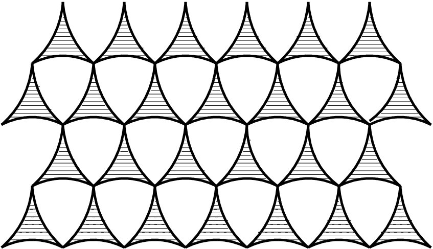

Wierman and Ziff [9] note that the reversed triangles must be connected in a specific manner to create a self-dual arrangement, and provide an example to illustrate that simply reversing each triangle is not sufficient.
II.2.2 Generators and Duality
A generator is a finite connected planar graph embedded in the plane so that three vertices on the infinite face are designated as boundary vertices A, B, and C. (For future research, the term generator may be defined more generally. However, in this paper, we restrict attention to generators with three boundary vertices.)
Given a generator , we construct its dual generator by placing a vertex in each bounded face of , and three vertices , , and of in the infinite face of , as follows: The boundary of the infinite face can be decomposed into three (possibly intersecting) paths, from to , to , and to . The infinite face may be partitioned into three infinite regions by three non-intersecting polygonal lines starting from , , and . Place in the region containing the boundary path connecting and , in the region containing the boundary path connecting and , and in the region containing the boundary path connecting and . , , and are the boundary vertices of .
For each edge of , construct an edge of which crosses and connects the vertices in the faces on opposite sides of . If is on the boundary of the infinite face, connect it to if is on the boundary path between and , to if is between and , and connect it to if is between and . (Note that it is possible for to connect more than one of , , and , for example, if there is a single edge incident to in , its dual edge connects and .)

Note that is not the dual graph of , which would have only one vertex in the infinite face. The three vertices , , and will correspond to separate faces of the lattice generated from .
II.2.3 Constructing a Dual Pair of Lattices
Given a planar generator and a connected periodic self-dual 3-uniform hypergraph , a dual pair of periodic lattices may be constructed as follows: Construct a lattice graph by replacing each hyperedge of H by a copy of the generator , with the boundary vertices of the generator corresponding to the vertices of the hyperedge, in such a manner that the resulting lattice is periodic. This is always possible, by choosing the orientations of the generator in one period of the hypergraph, and extending the choice periodically. (However, for a generator without sufficient symmetry, it may be possible to replace hyperedges in a way that produces a non-periodic lattice, so some care is needed.)
We now construct a lattice as follows: Construct the embedding of the dual hypergraph in the plane, in which every hyperedge of is reversed. Replace each hyperedge of by a copy of the dual generator , embedded so that it is consistent with the embedding of , that is, in all hyperedges boundary vertex in is opposite vertex in , is opposite , and is opposite , and each edge of crosses the appropriate edge of . (See Figure 2.) This results in a simultaneous embedding of and . An example of the construction for a particular generator is illustrated in Figure 3.


The constructions of the two lattices both produce a planar representation of the resulting lattice. From the simultaneous embeddings of the two lattices, it is seen that is the dual lattice of , since there is a one-to-one correspondence between vertices of one and faces of the other, and a one-to-one correspondence between edges, which are paired by crossing.
II.3 Substitution Method
Wierman [10] introduced the substitution method to find bounds on bond percolation critical probabilities for certain lattices. Its application to the martini class of lattices is described here. Let be a lattice constructed by placing copies of a generator in a self-dual 3-uniform hypergraph arrangement. A boundary vertex is a vertex that is in more than one copy of the generator. Let be the generator and suppose that its boundary vertices are , , and . Any configuration of open and closed bonds on gives a partition of the boundary vertices into connected open clusters of vertices. Vertical bars between the boundary vertices are used to denote such a partition. For example, denotes the partition where and are in the same open cluster and is in a separate open cluster.
II.3.1 Partially Ordered Sets
A partially ordered set, or briefly, a poset, consists of a pair , where is a set and is a binary relation with the following properties: (1) is reflexive, i.e., for all (2) is antisymmetric, i.e., for all and in , if and , then . (3) is transitive, i.e., for all ,, and in , if and , then .
In a partially ordered set , two elements of , and , are comparable if or , and are incomparable otherwise. A partially ordered set is a total order if every pair of its elements are comparable. For example, the standard relation on a set of real numbers is a total order. Partially ordered sets generalize the concept of total order by allowing incomparability. A common example of a partially ordered set that is not totally ordered is the set of all subsets, or power set, of a set of two or more elements with the relation of set inclusion, since some pairs of subsets are incomparable.
It is useful to have a visual representation of a partially ordered set. To efficiently represent a poset, it is useful to define the cover relationship. For , is covered by if and there is no element , unequal to both and , such that . The Hasse diagram of the partially ordered set is obtained by placing a point in the plane for each element of , taking care to put the point for below the point for whenever , and connecting the points for and by a line segment if and only if is covered by . Note that all other comparability relationships can be obtained from the covering relationships by following monotone paths in the Hasse diagram, so it is not necessary to complicate the diagram by including line segments for all pairs of comparable elements.
The set of boundary partitions of a generator is a partially ordered set, with, for boundary partitions and , whenever every cluster of can be decomposed into clusters of . In the previous example, , since is a decomposition of and is a trivial decomposition of . Equivalently, every cluster of is entirely contained in a single cluster of . Another equivalent condition is that every cluster of is a disjoint union of clusters of .

Figure 4 illustrates the Hasse diagram of a partially ordered set with 5 elements which is used throughout this article. The three middle partitions are pairwise incomparable, while all other pairs of partitions are comparable.
II.3.2 Stochastic Ordering
Stochastic ordering is used to compare two probability measures defined on the same partially ordered set. We will consider probability measures which are defined on the set of boundary partitions of a generator in terms of a bond percolation model on the generator. Consider a generator and a bond percolation model on with parameter . A configuration is a designation of each edge of as open or closed. In the percolation model, a configuration with open edges and closed edges has probability . A boundary partition is a union of configurations, with its probability being the sum of the probabilities of its configurations. Let denote the probability measure on boundary partitions of generated by the bond percolation model with parameter .
Let be a partially ordered set and let . is called an upset if for all and in , and imply that . If and are two probability measures on , we say is stochastically smaller than , denoted , if for all upsets of . This concept of stochastic ordering is the appropriate comparison of two probability measures on a partially ordered set when applying the substitution method [3].
In addition to a lattice , suppose another lattice is constructed by placing copies of a generator in the same self-dual 3-uniform hypergraph structure as The substitution method studies the effect on connection probabilities of replacing the generator of by the generator in .
Preston [11] established the equivalence of stochastic ordering and coupling for probability measures on finite partially ordered sets. For simplicity here, we will specialize to our percolation setting. If for two generators and , then there exist percolation models on and with parameters and respectively which are dependent on each other in such a manner that whenever boundary vertices are connected by open edges in they are also connected by open edges in . (Note that each percolation model corresponds to independently open edges in its generator, so is determined by its lattice connectivity, but that the realizations of the two percolation models are stochastically dependent upon each other.) In particular, the stochastic ordering implies that and . We use these consequences in section III, where solving for in the equations for all upsets allows us to obtain a stochastic ordering on the probability measures for a lattice and its dual near their percolation thresholds.
III Example: The Martini Lattice and Its Dual
In this section, we show that the critical exponents of the bond percolation models on the martini lattice and its dual, referred to as the lattice, are equal. The generators for the martini and lattices are shown in Figure 5. The method used is that introduced by Wierman [3] to show the equality of the bond percolation critical exponents for the triangular and hexagonal lattices and also for the bowtie lattice and its dual. There are no other cases where Wierman’s method has been used to show the equality of bond percolation critical exponents for dual lattices. This example is used as a reference in section IV, where the main result is shown. Precisely, we show that , , , and , where and refer to the martini and lattices respectively. So, if the limit defining the critical exponent exists for either lattice, it exists for both lattices and . Similarly, if the limit defining the critical exponent exists for either lattice, it exists for both lattices and . As in Wierman’s paper, the substitution method is used in this proof.

Ziff [6] was able to find the exact percolation threshold for the martini and lattices. A derivation of this threshold is summarized here. Let each bond in the lattice be open with probability . Then, the partition probabilites for the lattice can be calculated by conditioning on the bonds in the interior star:

Similarly, letting each bond be open in the martini lattice with probability , the partition probabilities for the martini lattice can be calculated by conditioning on the bonds in the triangle:

Using the substitution method, we replace each martini generator by the generator and set , , and . The second equation is satisfied when , which is a consequence of duality of the two lattices. The first and last equations are redundant, and give the following:
which has roots at . We thus have
that the critical probabilities are and
as shown before by Ziff [6].
To show equality of the bond percolation critical exponents, we will establish a stochastic ordering between the probability measures near and near . Specifically, we find that
by showing that
for all upsets of the poset of boundary partitions. This allows us to make conclusions about the behavior of the percolation probability near criticality. Proceeding, we equate the upset probabilities for the martini and lattices, keeping in mind that they are equal at criticality as a result of duality. The upset probability equations are given by:
for , where denotes the number of middle partitions in the upset. In studying critical exponents, we consider the behavior of the system near the percolation threshold, so we consider perturbations near and . Thus, we want to solve for in the following:
for .
Noting that the constant terms cancel out by the upset probability equations and letting
and
we see that
Using the approximation , the coefficients of are approximately:
for
for
for
for
Thus, for sufficiently small , is smaller than the coefficient in the solution for all four equations, and is larger than the coefficient in the solution for all four equations. Since the upset probability functions are increasing functions of the parameters, for sufficiently small positive , we have
for , and
for .
Each of these sets of inequalities establishes a stochastic ordering result. Thus, for sufficiently small ,
Using the result from Preston [11], we have that, for and sufficiently close to ,
Taking logarithms and dividing by throughout, we see that
Reversing this argument using gives:
Consequently, and, by changing limsup to liminf where it appears above,
we have that .
By the same reasoning, we also have that for sufficiently small ,
Thus, for with sufficiently close to ,
Letting gives that and .
IV Positive Coefficients for in the functions
In this section we generalize the result to lattices constructed
from an infinite connected planar periodic 3-uniform hypergraph with
one axis of symmetry, using a generator which is a finite connected
planar graph with three boundary vertices. See Wierman and Ziff
[9] for the construction of such lattices. As in section
III, the method used to show equality of the critical exponents is
valid if the coefficients of in the
functions are positive and finite. In this section we show that the
coefficients for lattices in the class are positive and finite. In
what follows, will denote the generator of a lattice in the
class of interest
and will denote its dual generator.
Calculate the coefficient of in the function as follows. First, equate the upset probabilites for the lattice and its dual, setting
,
where , , and take the values or .
Note that this is more general than the martini and
lattices example in that symmetry of the generator is not assumed.
The critical probabilities for the lattice and its dual are
then calculated using these equations. Adding to
and to in these equations shows how the
two functions behave around the critical probabilities.
Notice that the numerator of the coefficent of in the
martini and lattices example is the derivative of
and the denominator is the derivative of
. This holds for all generators in the
class. That is, the numerator of the coefficent of is the
derivative of
and the denominator is the derivative of
for any
generator in the class. This can be seen by the following
reasoning: Suppose the generator has bonds. Then, since the
lattice’s generator and its dual have the same number of bonds, the
expressions and
are polynomials
in and respectively with degree
no larger than . So, we can write
and
Equating these, and adding and to and respectively, yield the following:
Using binomial expansions, we can write this as:
Evaluating this at and , the constant terms on each side of this equation cancel as a result of the equality of the probability measures for dual lattices at criticality. Moreover, the coefficients of and are seen to be the derivatives of their respective upset probability functions. We thus have that
To show that the coefficient of epsilon is positive and finite,
it suffices to show that the derivatives of the upset probability
functions in both the lattice and its dual are positive on the
interval (0,1). Since the upset probability functions are polynomials,
their derivatives exist and are finite. If the derivatives are shown
to be positive, then they will be positive at and the coefficient
of will be positive, completing the argument.
We now prove that the derivatives of the partition probability functions for a lattice in the martini class and its dual are positive. Let be a minimal connected subgraph of the generator that contains , , and . Let denote the edge set of and let . is clearly a tree, so there is an unique path from to , from to , and from to . More importantly, removing any edge from makes connectivity between , , and impossible in .
We shall use the following notation for the proof. The superscript on the probability measure will indicate the structure for which the boundary vertices can be connected through; will indicate the generator of the lattice, will indicate the tree defined above, and will indicate through but not through . (The meaning of this will become clearer in the body of the proof.) Where no superscript appears, the statement is true for all three structures. The subscript will denote the probability of an edge being open in the graph. Where two subscripts appear, separated by a comma, the first subscript gives the probability that is open, and the second subscript gives the probability that each edge other than is open. may be defined differently in different cases, but will always be an edge in . Where no subscript appears, the statement is true for any subscript. It will be helpful to condition on being open or closed. A semicolon will separate the upset from the conditioning event. denotes the probability of the upset given that the edge is open, while denotes the probability of the upset given that the edge is closed.
Using this notation and continuing the discussion preceding the notational description, .
Let each bond in a lattice be open with probability , .
Let be an edge in , and therefore in , and let
, , …, be the other bonds in . Let
be independent uniform random variables on the
interval . For each realization of the
, if , call open. Otherwise,
is closed. Call this scenerio Model 1. Note that
denotes the probability that , , and are all connected in
in this case.
Consider the same lattice with the only difference being
that is open with probability .
Call this scenerio Model 2, and note that
denotes the probability that A, B, and C are all connected in this case.
The other partition probability functions are defined in this
case using the same subscript.
Call Model 3 the same as Model 1 with replaced by
in both the description and the notation. We use the same
realization in all three cases.
Notice that if an edge is open in Model 1, it is also open in Model 2.
So, if , , and are connected through open bonds in Model 1,
they are necessarily connected through open bonds in Model 2.
Also, if an edge is open in Model 2, it is open in Model 3 and
similar conclusions can be made.
In what follows, is the probability that , , and
are connected in only through , that is, they are not
connected if any edge of is closed. is the
probability that , , and are connected in , the
graph with edge deleted, for some edge We then
have that . We obtain a lower bound
on the derivative by considering the difference quotients:
Substituting
we see that the last expression above equals:
Since , , and the event that , , and are connected in with closed is contained in the event that the three are connected,
Similar reasoning is
valid for the other partition probability functions, one of which
will be given in detail here. Let , the
probability that and are connected in the lattice. Also,
let be an edge in on the unique path from to and
let be the number of edges in the path. Then,
,
In this way, it follows that all upset probability functions for a generator of a lattice in the class have a positive derivative in the interval (0,1). The exact same argument holds for the duals of these lattices, replacing by . Thus, the coefficient of used in this method to determine equality of the bond percolation critical exponents is well-defined and positive. As a consequence, any lattice and dual lattice in the class described have equal values for the two critical exponents and .
V Extensions and Generalizations
V.1 Other Critical Exponents
Additional percolation functions and critical exponents are considered in the literature.
Define the two-point connectivity function by:
, where “” denotes the event that the sites and are connected by an
open path.
Define the correlation length by
where ,
The critical exponents , , , and ,
for , are given by the power laws:
for some ,
, ,
for some ,
, , for some ,
and, for a -dimensional periodic graph,
, , for some .
In two dimensions, the values for the critical exponents defined in this paper are believed to be , , , and (See Grimmett [12] and Hughes [1]). Kesten [2] proved that for a class of two-dimensional periodic lattices (assuming the limits defining the exponents and exist), that
and that for all ,
The class of lattices considered by Kesten includes the lattices in the class identified by Wierman and Ziff.
We have already shown that and for any lattice in the given class. Furthermore, since and are equal, for all boundary vertices and . Thus, and decrease at the same exponential rate, so . Using Kesten’s formulas, equality of the other critical exponents is evident. That is, , , and .
Thus, the set of critical exponents are equal for a bond model and its dual in the given class. For example, the results apply to the lattice pairs mentioned in Ziff and Scullard [7]. Since each generator can appear in an infinite collection of self-dual hypergraphs, we have infinitely many lattices in which the set of critical exponents are equal.
Our results do not establish any numerical values for the critical exponents. However, remarkable progress in this direction was made by Smirnov and Werner [5], who combined Kesten’s scaling relations, knowledge of critical exponents associated with the stochastic Loewner evolution process, and Smirnov’s proof of conformal invariance to determine the existence and values of critical exponents for the site percolation model on the triangular lattice.
V.2 The Bowtie Lattice and Its Dual
By splitting each vertical bond in the bowtie lattice into two bonds, each having probability of being open, Wierman [3] used the substitution method to determine the critical probabilities of the bowtie lattice and its dual. The method described in this paper was then applied to this dual pair, showing the equality of their bond percolation critical exponents. Using this idea, the method described in this paper is applicable to many other lattices. In fact, as long as a lattice is self-dual under the triangle-triangle transformation (see Ziff and Scullard [7], and Wierman and Ziff [9]), functions of can be assigned as edge probabilities of a given lattice. That is, we can assign to each edge of the generator the probability of being open, where is an increasing, right-continuous function of . Under these conditions, repeating the main argument of the paper gives that, for any edge in the minimal tree connecting , , and ,
and it is clear that the coefficient of in the expression for is well-defined and positive. Equality of bond percolation critical exponents for such lattices and their duals follows from this fact.
V.3 Site Percolation
Since the bond problem of a lattice is equivalent to the site problem on its line lattice [4, 12, 13, 14], the result described in this paper applies to the collection of site problems obtained by reformulating the bond problems as site problems. As a result, we have a collection of site problems in which any lattice belonging to the collection shares the same value of its critical exponents with its matching lattice. So, for the bond model on any given lattice in the class identified by Wierman and Ziff, we can immediately identify three other lattices with the same values for the set of critical exponents: the bond model on the lattice’s dual, the corresponding site problem on the line lattice, and the site problem on the line lattice of the dual. Since each generator can appear in an infinite collection of self-dual hypergraphs, we have infinitely many site problems in which the set of critical exponents are equal.
The martini, A, and B lattices discussed in Scullard [8] are not line graphs of underlying lattices, so the results in the previous paragraph do not apply to the site percolation models on these lattices. It is plausible that the approach of this article may be applicable to such site percolation models, but that has not yet been shown to be valid, and is a subject of further study.
VI Concluding Remarks
The method used by Wierman to show equality of the bond percolation critical exponents for the triangle and hexagonal lattices was used to show the equality of the bond percolation critical exponents for the martini lattice and its dual. This computational proof was then extended to show that a lattice constructed from an infinite connected planar periodic 3-uniform hypergraph with one axis of symmetry, using a generator which is a finite connected planar graph with three boundary vertices, has the same values for its bond critical exponents as its dual, thereby generalizing the results of Wierman [3]. Since the mentioned class of lattices is infinite, there are infinitely many lattices that have the same bond percolation critical exponents as their duals. Moreover, since using the same generator on different self-dual hypergraphs does not affect the computations, there are an infinite number of bond and site models for which the critical exponents are the same. This result gives mathematical evidence that the values of the critical exponents may only depend on the dimension of the lattice, supporting the universality hypothesis. Note that the result does not say that the bond percolation critical exponents have the same value for all lattices in the mentioned class. Using different generators produces different upset probability functions, so no relations for the bond percolation critical exponents between generators has been determined. If two non-isomorphic, non-dual generators were discovered that had equal upset probability functions at criticality, the result could likely be extended to give equality of bond percolation critical exponents for these lattices. The authors of this paper have thus far been unable to identify two such generators.
References
- [1] B. D. Hughes, Random Walks and Random Environments (Oxford Science Publications, 1996), Vol. 2, pp. 284–290.
- [2] H. Kesten, Comm. in Math. Phys. 109, 109–156 (1987).
- [3] J. C. Wierman, Comb. Prob. Comp. 1 95–105 (1992).
- [4] H. Kesten, Percolation Theory for Mathematicians. (Birkhauser, Boston, 1982).
- [5] S. Smirnov and W. Werner, Math. Res. Lett. 8, 729–744 (2001)
- [6] R. M. Ziff, Phys. Rev. E 73, 016134 (2006).
- [7] R. M. Ziff and C. R. Scullard, Jour. Phys. A 39 15083–15090 (2006).
- [8] C. R. Scullard, Phys. Rev. E 73 016107 (2006).
- [9] J. C. Wierman and R. M. Ziff, Jour. Phys. A, submitted (arXiv:0903.3135) (2009).
- [10] J. C. Wierman, Disorder in Physical Systems (Oxford University Press, 1990) pp. 349–360.
- [11] C. J. Preston, Comm. Math. Phys. 36, 233–241 (1974).
- [12] G. Grimmett, Percolation, 2nd edition, (Springer, Berlin, 1999), p. 24.
- [13] M. E. Fisher, J. Math. Phys. 2, 620 (1961).
- [14] M. E. Fisher and J. W. Essam, J. Math. Phys. 2, 609 (1961).