Factorization and resummation for single color-octet scalar production at the LHC

Discovering the Higgs particle and the mechanism of electroweak symmetry breaking is one of the major goals of the Large Hadron Collider (LHC). It is well-known that the main Higgs production mechanism is the gluon-gluon fusion process. An important issue in determining the total production cross section is the large perturbative corrections in the threshold region, defined by $z\to 1$, where $z=m_{H}^{2}/\hat{s}$, where $m_{H}$ is the Higgs mass and $\hat{s}$ is the partonic center of mass energy squared. The leading corrections are enhanced by factors of ${\rm log}(1-z)/(1-z)$ and invalidate fixed order perturbation theory in the threshold region. These corrections can significantly affect the normalization of the total cross section even though the total cross section receives contributions from a range of $\hat{s}$ [1, 2, 3, 4]. In the threshold region, the inclusive scattering cross section $\sigma(pp\to HX)$ can be factorized (at leading twist) into a hard part, soft part, and parton distribution function (PDF) of gluons inside the proton [5], and the renormalization group equations (RGE) for these parts can be used to resum the large threhold corrections. For the Higgs production cross section the calculations up to the next-to-next-leading logarithm (NNLL) accuracy have already been performed [5, 6] and give total cross section about three times bigger than predicted at leading order.

Obviously, properly incorporating these effects will be important for other heavy particles predicted in theories of New Physics (NP) that may be observed at the LHC. In this paper we will focus on the production of a heavy color-octet scalar, which appears in a number of NP models such as grand unified theories [7, 8, 9], supersymmetric theories [10, 11], Pati-Salam unification [12, 13], chiral color [14], and topcolor [15]. We will calculate the cross section for the Manohar-Wise model [16] of color-octet scalars which is consistent with the principle of Minimal Flavor Violation (MFV) [17, 18]. Performing the resummation for color-octet scalars is very similar to the resummation for Higgs [1, 3, 4]. Similar resummations have been performed for squark-antisquark and gluino-pair production cross sections in Refs.  [19, 20]. We will use Soft-Collinear Effective Theory (SCET) [21, 22, 23] to derive a factorization theorem for the cross section. Gluon-gluon fusion cross sections in the full theory are matched onto SCET operators. The matching coefficients for these operators will differ between various models, but the structure of these operators is universal. The cross section computed with the SCET operators factors into correlation functions of SCET collinear and soft fields, and renormalization group equations for these correlation functions can be used to perform the resummation of the threshold logarithms. This resummation procedure is independent of the NP model.

Before we discuss the factorization theorem, we will describe some details of the color-octet scalar model we will be focusing on. The principle of MFV requires that the Yukawa couplings of the color-octet scalars be proportional to the Yukawa matrices in the Standard Model. The Standard Model Yukawa couplings are

$\displaystyle{\cal L}=-\,g_{ij}^{D}\bar{d}_{Ri}H^{\dagger}Q_{Lj}-\,g_{ij}^{U}\bar{u}_{Ri}\epsilon H^{*}Q_{Lj}+h.c.\,,$

(1)

where $Q_{L}$ is the doublet of lefthanded quarks, $u_{R}$ and $d_{R}$ are the righthanded up and down quarks, respectively, $i$ and $j$ are flavor indices, and $H$ is the Higgs doublet:

$\displaystyle H=\left(\begin{array}[]{c}H^{+}\\ H^{0}\end{array}\right)\qquad\epsilon H^{*}=\left(\begin{array}[]{c}H^{0*}\\ -H^{-}\end{array}\right)\,.$

If the color-octet scalar Yukawa couplings are

$\displaystyle{\cal L}=-\,\lambda_{ij}^{D}\bar{d}_{Ri}S^{a\dagger}T^{a}Q_{Lj}-\,\lambda_{ij}^{U}\bar{u}_{Ri}\epsilon S^{a*}T^{a}Q_{Lj}\,,+h.c.\,.$

(7)

then the MFV hypothesis requires $\lambda_{ij}^{U,D}=\eta_{U,D}\,g^{U,D}_{ij}$, where $\eta_{U,D}$ are constants. This eliminates tree-level flavor changing neutral currents and ensures that experimental constraints from flavor physics are not violated. Note that this also implies that the $S^{a}$ couple most strongly to the third generation of quarks. The color-octet scalars have gauge couplings to gluons and a gauge invariant mass term

$\displaystyle\mathcal{L}_{\mathrm{QCD}}=-\frac{1}{2}S^{a}(D^{2})^{ac}S^{c}-\frac{1}{2}m_{S}^{2}S^{a}S^{a}\,,$

(8)

where $D_{\mu}^{ac}=\partial_{\mu}\delta^{ac}+gf^{abc}A_{\mu}^{b}$. Finally, there is a scalar potential for the $S^{a}$ and the Higgs that can be found in Ref. [16].

Though it may seem ad hoc to impose $\lambda_{ij}^{U,D}\propto\,g^{U,D}_{ij}$, this can arise naturally in certain models. For example, consider the chiral color model of Ref. [14]. In this model, the gauge group is enlarged to $SU(3)_{L}\times SU(3)_{R}\times SU(2)_{L}\times U(1)_{Y}$, and the chiral color group $SU(3)_{L}\times SU(3)_{R}$ breaks down to $SU(3)_{c}$ at some high energy scale. If the righthanded quarks are placed in the $(1,3,1)$ representation of $SU(3)_{L}\times SU(3)_{R}\times SU(2)_{L}$, and the lefthanded quarks are placed in the $(3,1,2)$, then quarks can obtain masses from the following Yukawa couplings

$\displaystyle{\cal L}=-\,\sqrt{3}\,g_{ij}^{D}\bar{d}_{Ri}\Phi^{\dagger}Q_{Lj}-\,\sqrt{3}\,g_{ij}^{U}\bar{u}_{Ri}\epsilon\Phi^{\prime*}Q_{Lj}+h.c.\,,$

(9)

where $\Phi$ and $\Phi^{\prime}$ transform in the $(3,\bar{3},2)$ and $(\bar{3},3,2)$, respectively.¹¹ 1 Note that an additional scalar in the $(1,1,2)$ is required to give masses to leptons. The fields $\Phi$, $\Phi^{\prime}$ can be decomposed into singlet and octet scalars under the unbroken $SU(3)_{c}$.

$\displaystyle\Phi^{(\prime)}=\frac{1}{\sqrt{3}}H^{(\prime)}+S^{a(\prime)}T^{a}$

(10)

and $\lambda_{ij}^{U,D}=\sqrt{3}\,g^{U,D}_{ij}$ at tree level. Note that this model is different from the Manohar-Wise model since there are two distinct color-octet scalars, $S^{a}$ and $S^{a\prime}$. If the gluon-gluon fusion production of a single color-octet scalar proceeds through a top-quark loop, this mechanism will predominantly produce $S^{a\prime}$. We do not wish to to study this model further, but mention it to show that the MFV constraint $\lambda_{ij}^{U,D}\propto\,g^{U,D}_{ij}$ could emerge as a consequence of a symmetry of the underlying theory.

The color-octet scalars can be produced via the pair production cross section, $gg\to SS$ which proceeds through gauge couplings [16]. Constraints on pair production followed by decay to heavy quarks has been used to establish a lower bound on $m_{S}$ of about $200$ GeV in Ref. [25]. Neutral color-octet scalars can also be produced singly via gluon-gluon fusion [24]. This proceeds through loop diagrams containing quarks, of which the top quark gives by far the dominant contribution, and loops with color-octet scalars. The relative size of the top quark and scalar loop contributions is determined by $\eta_{U}$ and other parameters in the scalar potential. If these parameters are all taken to be of order unity then the top quark loop is the largest contribution. ²² 2 If the color-octet is a pseudoscalar only the top quark loop contributes. In this case the production mechanism is very similar to that for a single Higgs, and hence threshold corrections are expected to be significant. At the LHC the production cross section for single $S$ production is larger than pair production when the mass of $S$ is larger than 1 TeV [24].

When applying SCET to color-octet scalar production we first match full QCD onto SCET operators at the hard scale $\mu_{h}\sim m_{S}$, where $m_{S}$ is the mass of the color-octet field. SCET is formulated as an expansion in $\lambda\sim\sqrt{\mu_{s}/\mu_{h}}$, where $\mu_{s}$ is the soft scale, $\mu_{s}\sim m_{S}(1-z)$. The allowed SCET operators are constrained by SCET gauge symmetries [26]. At leading order in $\lambda$, we find two dimension-5 operators with different color structures. Subleading operators will be constrained by the requirement of reparametrization invariance [27].

Our result for the factorized scattering cross section is

$\displaystyle\sigma(pp\to SX)$

$\displaystyle=$

$\displaystyle\tau H(m_{S},\mu_{f})\int^{1}_{\tau}\frac{dz}{z}\bar{S}(m_{S}(1-z),\mu_{f})F(\tau/z,\mu_{f}).$

(11)

Here $\tau=m_{S}^{2}/s$ where $s$ is the center of mass energy squared at the LHC, $H(m_{S},\mu)$ and $\bar{S}(m_{S}(1-z),\mu)$ are the hard and soft functions respectively, and $F(x,\mu)$ is the following convolution of the gluon PDF’s:

$$F(x,\mu_{f})=\int^{1}_{x}\frac{dy}{y}f_{g/P}(y,\mu_{f})f_{g/P}(x/y,\mu_{f}).$$

(12)

Renormalization group equations for the $H(m_{S},\mu_{f})$, $\bar{S}(m_{S}(1-z),\mu_{f})$, and $F(\tau/z,\mu_{f})$ can be used to resum large threshold corrections as will be discussed below.

In order to prove the factorization theorem in Eq. (11) we need to construct the SCET operators composed of the collinear gluons from the initial state hadrons, soft gluons, and a heavy color-octet scalar field. In the center of the mass frame, the incoming gluons from the two incoming protons are described as $n$ and $\overline{n}$-collinear fields where the light-cone vectors satisfy $n^{2}=\overline{n}^{2}=0,~n\cdot\overline{n}=2$. The lowest dimension operator with a single $n$-collinear gluon that is $n$-collinear gauge invariant is $W_{n}^{\dagger}G_{n}^{\mu\nu}W_{n}$. Here $G_{n}^{\mu\nu}=G_{n}^{a,\mu\nu}T^{a}$ is a SCET gluon field strength tensor, and $W_{n}$ is the collinear Wilson line

$$W_{n}(x)=\mathrm{P}\exp\Biggl(ig\int^{x}_{-\infty}ds~\overline{n}\cdot A_{n}^{a}(s\overline{n}^{\mu})T^{a}\Biggr).$$

(13)

Similarly, the lowest dimension $\overline{n}$-collinear gauge invariant operator is $W_{\overline{n}}^{\dagger}G_{\overline{n}}^{\mu\nu}W_{\overline{n}}$. Combining $W_{n}^{\dagger}G_{n}^{\mu\nu}W_{n}$ and $W_{\overline{n}}^{\dagger}G_{\overline{n}}^{\mu\nu}W_{\overline{n}}$ into a Lorentz scalar and then expanding to lowest order in $\lambda$ yields

	$\displaystyle\Bigl(W_{n}^{\dagger}G_{n}^{\mu\nu}W_{n}\Bigr)_{\alpha\beta}\Bigl(W_{\overline{n}}^{\dagger}G_{\overline{n},\mu\nu}W_{\overline{n}}\Bigr)_{\gamma\delta}$	$\displaystyle=$	$\displaystyle-\frac{1}{g^{2}}\Bigl(W_{n}^{\dagger}[iD_{n}^{\mu},iD_{n}^{\nu}]W_{n}\Bigr)_{\alpha\beta}\Bigl(W_{\overline{n}}^{\dagger}[iD_{\overline{n}\mu},iD_{\overline{n}\nu}]W_{\overline{n}}\Bigr)_{\gamma\delta}$		(14)
		$\displaystyle=$	$\displaystyle-\Bigl(\mathcal{B}_{n}^{\perp\mu}\Bigr)_{\alpha\beta}\Bigl(\mathcal{B}_{\overline{n},\mu}^{\perp}\Bigr)_{\gamma\delta}+\mathcal{O}(\lambda).$

Here $\alpha,\beta,\gamma$, and $\delta$ are color indices in the fundamental representation and $\mathcal{B}_{n}^{\perp\mu}$ is

$$\mathcal{B}_{n}^{\perp\mu}=\frac{1}{g}\Bigl[\overline{n}\cdot\mathcal{P}W_{n}^{\dagger}iD_{n}^{\perp\mu}W_{n}\Bigr],$$

(15)

where the derivative operator $\mathcal{P}^{\mu}$ returns the large label momentum and only acts on collinear fields within the brackets $[\cdots]$. It will be convenient to write the field $\mathcal{B}_{n}^{\perp\mu}$ in terms of the Wilson line in the adjoint representation (i.e. with color generator $(t^{a})_{bc}=-if^{abc}$). Defining $\mathcal{B}_{n}^{\perp\mu}=\mathcal{B}_{n\perp}^{a,\mu}T^{a}$, $\mathcal{B}_{n\perp}^{a,\mu}$ is given by

$$\mathcal{B}_{n\perp}^{a,\mu}=i\overline{n}^{\rho}g_{\perp}^{\mu\nu}\mathcal{W}_{n}^{\dagger,ab}G_{n,\rho\nu}^{b}=i\overline{n}^{\rho}g_{\perp}^{\mu\nu}G_{n,\rho\nu}^{b}\mathcal{W}_{n}^{ba},$$

(16)

where $\mathcal{W}_{n}$ is the collinear Wilson line in the adjoint representation, and we used the relation $\mathcal{W}_{n}^{ab}=\mathcal{W}_{n}^{\dagger ba}$ for the second equality. For the $\overline{n}$-collinear fields, $\mathcal{B}_{\overline{n}}^{\perp\mu}$ and $\mathcal{B}_{\overline{n}\perp}^{a,\mu}$ are identical to $\mathcal{B}_{n}^{\perp\mu}$ and $\mathcal{B}_{n\perp}^{a,\mu}$, respectively, after interchanging $n$ and $\overline{n}$.

Finally, we need to include fields for the color-octet scalar. The strong interactions of this field are described by Eq. (8). At scales well below $m_{S}$, the strong interactions of the heavy color-octet scalar simplify because the scalar is slowly moving. In the threshold region, the $S^{a}$ is produced nearly at rest (in the parton center-of-mass frame) and heavy particle effective theory techniques can be applied. We use a heavy scalar effective theory (HSET), similar to heavy quark effective theory (HQET). In HSET, the scalar momentum is decomposed into large and small parts: $p^{\mu}_{S}=m_{S}v^{\mu}+k^{\mu}$, where $v^{\mu}$ is the static four-velocity and $k^{\mu}$ represents fluctuations of $O(\mu_{s})$. In order for derivatives in HSET to bring factors of $k^{\mu}$ rather than the total momentum, we use the standard rephasing trick to relate full theory and HSET fields :

$$S^{a}(x)=\frac{1}{\sqrt{2m_{S}}}\Bigl(e^{-im_{S}v\cdot x}S_{v}^{a}(x)+e^{im_{S}v\cdot x}S_{v}^{*a}(x)\Bigr).$$

(17)

The HSET Lagrangian is obtained by plugging Eq. (17) into Eq. (8) and taking the large $m_{S}$ limit, in which the only surviving terms are those for which the phase factor cancels. We find

$$\mathcal{L}_{\mathrm{HSET}}=S_{v}^{*a}(v\cdot iD_{s})^{ac}S_{v}^{c}-\frac{1}{2m_{S}}S_{v}^{*a}(D_{s}^{2})^{ac}S_{v}^{c},$$

(18)

where $v^{\mu}$ is the four-velocity and the covariant derivative, $D^{\mu}_{s}$, involves only soft gluons. The first term in Eq. (18) gives the leading interactions, and the second term is suppressed by $1/m_{S}$ and so can be neglected.

In our SCET-HSET operators, the soft gluons appear in the soft Wilson lines,

$$\mathcal{Y}_{\mathrm{v}}(x)=\mathrm{P}\exp\Biggl(ig\int^{x}_{-\infty}ds~\mathrm{v}\cdot A_{s}^{a}(s\mathrm{v}^{\mu})t^{a}\Biggr),$$

(19)

where $\rm{v}^{\mu}$ can be either $n^{\mu}$, $\overline{n}^{\mu}$, or $v^{\mu}$. These soft Wilson lines arise when we decouple the leading soft interactions from the collinear and heavy scalar fields by the field redefinitions [22]

	$\displaystyle A_{n}^{a,\mu}\to\mathcal{Y}_{n}^{ab}A_{n}^{b,\mu},~~~\mathcal{W}_{n}^{(\dagger)ab}\to\mathcal{Y}_{n}^{ac}\mathcal{W}_{n}^{(\dagger)cb}$		(20)
	$\displaystyle A_{\overline{n}}^{a,\mu}\to\mathcal{Y}_{\overline{n}}^{ab}A_{\overline{n}}^{b,\mu},~~~\mathcal{W}_{\overline{n}}^{(\dagger)ab}\to\mathcal{Y}_{\overline{n}}^{ac}\mathcal{W}_{\overline{n}}^{(\dagger)cb}$
	$\displaystyle S_{v}^{a}\to\mathcal{Y}_{v}^{ab}S_{v}^{b},~~~S_{v}^{*a}\to\mathcal{Y}_{v}^{ba}S_{v}^{*b}.$

After this field redefinition, the collinear fields and HSET fields do not interact with the soft particles. Note that after the field redefinition, $\mathcal{L}_{\rm{HSET}}=S_{v}^{a*}(v\cdot i\partial)S^{a}_{v}+O(1/m_{S})$, so the strong interactions vanish at leading order in $O(1/m_{S})$. The heavy scalar’s interaction with soft gluons can be reproduced by a soft Wilson line. This replacement simplifies the derivation of the factorization theorem as we show below.

Using $\mathcal{B}_{n}^{\perp\mu}$, $\mathcal{B}_{\overline{n}}^{\perp\mu}$, $S^{a}_{v}$, and the soft Wilson lines we can construct the effective Lagrangian for color-octet production at leading order in $\lambda$,

$$\mathcal{L}_{\mathrm{SCET}}=C_{S}(\mu)O_{S}(\mu)+C_{P}(\mu)O_{P}(\mu),$$

(21)

where the effective theory operators $O_{S}$ and $O_{P}$ are for color-octet scalars ($S_{S}$) and pseudoscalars ($S_{P}$) respectively. Those operators have different color structures and are

	$\displaystyle O_{S}$	$\displaystyle=$	$\displaystyle\frac{d^{abc}}{\sqrt{2m_{S}}}(S_{Sv}^{*}\mathcal{Y}_{v}^{\dagger})^{a}(\mathcal{B}_{\overline{n}}^{\perp\mu}\mathcal{Y}_{\overline{n}}^{\dagger})^{b}(\mathcal{Y}_{n}\mathcal{B}_{n\mu}^{\perp})^{c},$		(22)
	$\displaystyle O_{P}$	$\displaystyle=$	$\displaystyle\frac{if^{abc}}{\sqrt{2m_{S}}}\epsilon^{\perp}_{\mu\nu}(S_{Pv}^{*}\mathcal{Y}_{v}^{\dagger})^{a}(\mathcal{B}_{\overline{n}}^{\perp\mu}\mathcal{Y}_{\overline{n}}^{\dagger})^{b}(\mathcal{Y}_{n}\mathcal{B}_{n}^{\perp\nu})^{c},$		(23)

where $\epsilon^{\perp}_{\mu\nu}=\epsilon_{\mu\nu\rho\sigma}n^{\rho}\overline{n}^{\sigma}/2$. Note that the strong interaction Lagrangian for the pseudoscalar is the same as the scalar. Since the $n$-collinear, $\overline{n}$-collinear, and the soft fields are decoupled, the renormalization of the both operators will be a simple product given by

$\displaystyle Z_{S,P}=Z_{\mathcal{Y}}\,Z_{n}\,Z_{\overline{n}}\,,$

(24)

where $Z_{n}$ and $Z_{\overline{n}}$ are the renormalization factors for the collinear parts $\mathcal{B}_{n}^{\perp\mu}$ and $\mathcal{B}_{\overline{n}}^{\perp\mu}$, respectively, and $Z_{\mathcal{Y}}$ is the renormalization factor for the three soft Wilson lines. So the renormalizations of $O_{S}$ and $O_{P}$ are the same and do not depend on either color structure constants or the Lorentz structure. Therefore, below we only consider the renormalization of the scalar operators, however our results hold for pseudoscalar operators as well.

Taking the matrix elements of $C_{S}(\mu)O_{S}(\mu)$ in Eq. (21), we find the scattering cross section

	$\displaystyle\sigma(pp\to S_{S}X)$	$\displaystyle=$	$\displaystyle\frac{\pi}{s}\sum_{X}\int d^{4}q\delta(q^{2}-m_{S}^{2})\delta(P_{n}+P_{\overline{n}}-q-p_{X})$
			$\displaystyle\times|C_{S}(m_{S},\mu)|^{2}\langle P_{n}P_{\overline{n}}|O_{S}^{\dagger}(\mu)|S_{S}X\rangle\langle S_{S}X|O_{S}(\mu)|P_{n}P_{\overline{n}}\rangle,$

where $P_{n}^{\mu}$ and $P_{\overline{n}}^{\mu}$ are the momenta of the incoming protons which are $n$-collinear and $\overline{n}$-collinear, respectively. Because the final state $X$ consists of $n(\overline{n})$-collinear and soft states in the partonic threshold region, it is possible to rewrite the final state summation as $\sum_{X}=\sum_{X_{n}}\sum_{X_{\overline{n}}}\sum_{X_{S}}$ and the final state momentum $p_{X}=p_{X_{n}}+p_{X_{\overline{n}}}+p_{X_{S}}$. The momentum of the color-octet field is

$$q=P_{n}+P_{\overline{n}}-(p_{X_{n}}+p_{X_{\overline{n}}}+p_{X_{S}})=p_{n}+p_{\overline{n}}-p_{X_{S}},$$

(25)

where $p_{n}=P_{n}-p_{X_{n}}$ and $p_{\overline{n}}=P_{\overline{n}}-p_{X_{\overline{n}}}$ are momenta of the partons in the two incoming protons. Then the argument in the first delta function in Eq. (Factorization and resummation for single color-octet scalar production at the LHC) is

	$\displaystyle q^{2}-m_{S}^{2}$	$\displaystyle=$	$\displaystyle(p_{n}+p_{\overline{n}}-p_{X_{S}})^{2}-m_{S}^{2}\sim(p_{n}+p_{\overline{n}})^{2}-2p_{X_{S}}\cdot(p_{n}+p_{\overline{n}})-m_{S}^{2}$		(26)
		$\displaystyle=$	$\displaystyle\hat{s}-2\eta\hat{s}^{1/2}-m_{S}^{2},$

where $\eta=p_{X_{S}}^{0}$ is the energy carried by final state soft particles in the partonic center-of-mass frame, and $\hat{s}=\overline{n}\cdot p_{n}n\cdot p_{\overline{n}}=y_{1}y_{2}s$, where $y_{1,2}$ are the large (collinear) momentum fractions of the incoming partons, defined by $y_{1}=\overline{n}\cdot p_{n}/\overline{n}\cdot P_{n}$ and $y_{2}=n\cdot p_{\overline{n}}/n\cdot P_{\overline{n}}$. When the momentum $q$ is on-shell, Eq. (26) implies

$$\eta=\frac{\hat{s}-m_{S}^{2}}{2\hat{s}}=\frac{\hat{s}(1-z)}{2}=\frac{m_{S}(1-z)}{2z^{1/2}}\sim\frac{m_{S}(1-z)}{2},$$

(27)

where the last approximation is valid in the limit $z=m_{S}^{2}/\hat{s}=\tau/(y_{1}y_{2})\to 1$.

The cross section in Eq. (Factorization and resummation for single color-octet scalar production at the LHC) can be factorized by first inserting the identity

$\displaystyle 1=\int d\eta dy_{1}dy_{2}\delta(\eta+i\partial_{0})\delta\left(y_{1}-\frac{\overline{n}\cdot\mathcal{P}}{\overline{n}\cdot P_{n}}\right)\delta\left(y_{2}-\frac{n\cdot\mathcal{P}}{n\cdot P_{\overline{n}}}\right),$

(28)

where $\overline{n}\cdot\mathcal{P}$ is a label operator acting on $n$-collinear fields, $n\cdot\mathcal{P}$ is a label operator acting on $\overline{n}$-collinear fields, and the partial derivative, $i\partial_{0}$, acts only on soft fields. Then $\sigma(pp\to S_{S}X)$ can be written as

	$\displaystyle\sigma(pp\to S_{S}X)$	$\displaystyle=$	$\displaystyle\frac{\pi}{s}\int d\eta dy_{1}dy_{2}\delta\Bigl(\eta-\frac{m_{S}(1-z)}{2}\Bigr)\frac{|C_{S}(m_{S},\mu)|^{2}}{2\hat{s}^{1/2}}$		(29)
			$\displaystyle\times\frac{d^{abc}d^{def}}{2m_{S}}\Bigl\langle P_{n}P_{\overline{n}}\Bigl|(\mathcal{Y}_{v}S_{Sv})^{a}(\mathcal{B}_{n}^{\perp\mu}\mathcal{Y}_{n}^{\dagger})^{b}(\mathcal{Y}_{\overline{n}}\mathcal{B}_{\overline{n}\mu}^{\perp})^{c}\Bigr|S_{S}X\Bigr\rangle$
			$\displaystyle\times\Bigl\langle S_{S}X\Bigl|\delta(\eta+i\partial_{0})(S_{Sv}^{*}\mathcal{Y}_{v}^{\dagger})^{d}(\mathcal{B}_{\overline{n}\mu}^{\perp}[y_{2}]\mathcal{Y}_{\overline{n}}^{\dagger})^{e}(\mathcal{Y}_{n}\mathcal{B}_{n\mu}^{\perp}[y_{1}])^{f}\Bigr|P_{n}P_{\overline{n}}\Bigr\rangle.$

The cross section $\sigma(pp\to S_{P}X)$ is the same up to the color factor and the replacement $C_{S}(m_{S},\mu)\to C_{P}(m_{S},\mu)$. Then we use $S_{v}^{a}|S\rangle=\sqrt{2m_{S}}\epsilon^{a}$ and $\langle S|S_{v}^{*b}=\sqrt{2m_{S}}\epsilon^{*b}$ to remove the color-octet scalar from the final state, where $\epsilon^{a}$ are color polarization vectors satisfying the relations, $\sum_{pol}\epsilon^{*a}\epsilon^{b}=\delta^{ab}$. Finally, we apply the completeness relation, $1=\sum_{X}|X\rangle\langle X|$. After these manipulations, we find that $\sigma(pp\to S_{S}X)$ is given by

	$\displaystyle\sigma(pp\to S_{S}X)$	$\displaystyle=$	$\displaystyle\frac{\pi d^{abc}d^{def}}{s}\int dy_{1}dy_{2}\frac{|C_{S}(m_{S},\mu)|^{2}}{2\hat{s}^{1/2}}\Bigl\langle P_{n}P_{\overline{n}}\Bigl|\mathcal{Y}_{v}^{ak}\mathcal{B}_{n}^{\perp\mu,l}\mathcal{Y}_{n}^{\dagger lb}\mathcal{Y}_{\overline{n}}^{cm}\mathcal{B}_{\overline{n}\mu}^{\perp,m}$		(30)
			$\displaystyle\times\delta\Bigl(\frac{m_{S}(1-z)}{2}+i\partial_{0}\Bigr)\mathcal{Y}_{v}^{\dagger kd}\mathcal{B}^{\perp,n}_{\overline{n},\nu}[y_{2}]\mathcal{Y}_{\overline{n}}^{\dagger ne}\mathcal{Y}_{n}^{fo}\mathcal{B}^{\perp\nu,o}_{n}[y_{1}]\Bigr|P_{n}P_{\overline{n}}\Bigr\rangle.$

To simplify the notation we have defined

$$\mathcal{B}^{\perp\mu,a}_{n}[y_{1}]=\Bigl[\delta\Bigl(y_{1}-\frac{\overline{n}\cdot\mathcal{P}}{\overline{n}\cdot P_{n}}\Bigr)\mathcal{B}^{\perp\mu,a}_{n}\Bigr],~~~\mathcal{B}^{\perp\mu,a}_{\overline{n}}[y_{2}]=\Bigl[\delta\Bigl(y_{2}-\frac{n\cdot\mathcal{P}}{n\cdot P_{\overline{n}}}\Bigr)\mathcal{B}^{\perp\mu,a}_{\overline{n}}\Bigr].$$

(31)

The PDF for the $n$-collinear proton in terms of SCET fields is

	$\displaystyle f_{g/P_{n}}(x)$	$\displaystyle=$	$\displaystyle\frac{1}{2\pi x\overline{n}\cdot P_{n}}\int\frac{dn\cdot z}{2}e^{-ix\overline{n}\cdot P_{n}n\cdot z/2}$		(32)
			$\displaystyle\times\overline{n}^{\alpha}\overline{n}^{\beta}g_{\perp}^{\mu\nu}\Bigl\langle P_{n}\Bigl|G_{n,\alpha\mu}^{a}\left(\frac{n\cdot z}{2}\right)\mathcal{W}_{n}^{ab}\Bigl[\frac{n\cdot z}{2},0\Bigr]G^{b}_{n,\beta\nu}(0)\Bigr|P_{n}\Bigr\rangle$
		$\displaystyle=$	$\displaystyle\frac{1}{x\overline{n}\cdot P_{n}}\overline{n}^{\alpha}\overline{n}^{\beta}g_{\perp}^{\mu\nu}\Bigl\langle P_{n}\Bigl|G_{n,\alpha\mu}^{a}\mathcal{W}_{n}^{ab}\delta(x\overline{n}\cdot P_{n}-\overline{n}\cdot\mathcal{P})\mathcal{W}_{n}^{\dagger bc}G^{c}_{n,\beta\nu}\Bigr|P_{n}\Bigr\rangle$
		$\displaystyle=$	$\displaystyle\frac{1}{x(\overline{n}\cdot P_{n})^{2}}\Bigl\langle P_{n}\Bigl|\mathcal{B}_{n\perp}^{a,\mu}\delta\Bigl(x-\frac{\overline{n}\cdot\mathcal{P}}{\overline{n}\cdot P_{n}}\Bigr)\mathcal{B}_{n\mu}^{\perp,a}\Bigr|P_{n}\Bigr\rangle$

where $P_{n}^{\mu}$ is the momentum of the proton. Here, we have defined $\mathcal{W}_{n}^{ab}[z,0]=\mathcal{W}_{n}^{ab}(z)\mathcal{W}_{n}^{\dagger bc}(0)$ and used Eq. (16) for the third equality. A similar set of manipulations yields the PDF for the $\overline{n}$-collinear proton, and since $f_{g/P_{n}}(x)=f_{g/P_{\overline{n}}}(x)$, we will drop the subscripts $n$ and $\overline{n}$ in what follows. Therefore, after averaging over proton spins in Eq. (30), we find

	$\displaystyle\langle P_{n}|\mathcal{B}_{n}^{\perp\mu,l}\mathcal{B}_{n}^{\perp\nu,o}[y_{1}]|P_{n}\rangle$	$\displaystyle=$	$\displaystyle g_{\perp}^{\mu\nu}\delta^{lo}\frac{y_{1}(\overline{n}\cdot P_{n})^{2}}{2(N_{c}^{2}-1)}f_{g/P}(y_{1}),$		(33)
	$\displaystyle\langle P_{\overline{n}}|\mathcal{B}_{\overline{n}\mu}^{\perp,m}\mathcal{B}_{\overline{n}\nu}^{\perp,n}[y_{2}]|P_{\overline{n}}\rangle$	$\displaystyle=$	$\displaystyle g^{\perp}_{\mu\nu}\delta^{mn}\frac{y_{2}(n\cdot P_{\overline{n}})^{2}}{2(N_{c}^{2}-1)}f_{g/P}(y_{2}).$

The soft function $\bar{S}_{S}~(\bar{S}_{P})$ for the scalar (pseudoscalar) production is defined to be

	$\displaystyle\bar{S}_{S}(m_{S}(1-z))$	$\displaystyle=$	$\displaystyle\frac{3d^{abc}d^{def}}{40}\Bigl\langle 0\Bigl|\mathcal{Y}_{v}^{ak}\mathcal{Y}_{n}^{bl}\mathcal{Y}_{\overline{n}}^{cm}\delta\Bigl(1-z+2\frac{i\partial_{0}}{m_{S}}\Bigr)\mathcal{Y}_{v}^{\dagger kd}\mathcal{Y}_{n}^{\dagger le}\mathcal{Y}_{\overline{n}}^{\dagger mf}\Bigr|0\Bigr\rangle,$		(34)
	$\displaystyle\bar{S}_{P}(m_{S}(1-z))$	$\displaystyle=$	$\displaystyle\frac{f^{abc}f^{def}}{24}\Bigl\langle 0\Bigl|\mathcal{Y}_{v}^{ak}\mathcal{Y}_{n}^{bl}\mathcal{Y}_{\overline{n}}^{cm}\delta\Bigl(1-z+2\frac{i\partial_{0}}{m_{S}}\Bigr)\mathcal{Y}_{v}^{\dagger kd}\mathcal{Y}_{n}^{\dagger le}\mathcal{Y}_{\overline{n}}^{\dagger mf}\Bigr|0\Bigr\rangle.$		(35)

Here, the soft functions are normalized to $\delta(1-z)$ at lowest order.

Using these definitions we obtain the factorized scattering cross sections which are given by

$$\sigma(pp\to S_{i}X)=\tau H_{i}(m_{S},\mu_{f})\int^{1}_{\tau}\frac{dz}{z}\bar{S}_{i}(m_{S}(1-z),\mu_{f})F(\tau/z,\mu_{f}),~~~i=S,P,$$

(36)

where the hard coefficients $H_{i}$ are

$$H_{S}(m_{S},\mu_{f})=\frac{5\pi|C_{S}(m_{S},\mu_{f})|^{2}}{48},~~~H_{P}(m_{S},\mu_{f})=\frac{3\pi|C_{P}(m_{S},\mu_{f})|^{2}}{16}.$$

(37)

This factorization theorem is our main result. When we consider the renormalization group evolution effects, we will calculate $H_{S,P}(m_{S},\mu)~(\bar{S}_{S,P}(m_{S}(1-z),\mu))$ at the scale $\mu_{h}~(\mu_{s})$ and then evolve them to the factorization scale $\mu_{f}$. At the leading order (LO) in $\alpha_{s}$, the cross section is

$\displaystyle\sigma(pp\to S_{i}X)=\tau H_{i}^{(0)}F(\tau),~~~i=S,P,$

(38)

where $H_{i}^{(0)}$ are the hard coefficient at the lowest order and are equal to the scattering cross section at the Born level.

Next we discuss the RGE evolution of the hard and soft parts and the resummation of the cross section. Once the evolution for the coefficient functions, $C_{S,P}(\mu)$, is determined, the evolution equation for the soft function can be easily derived, since the evolution equations for $f_{g/p}(x)$ are known. The evolution of the soft functions can be done in momentum space as in the analysis of Higgs production and Drell-Yan in Refs. [2, 3, 4]. We follow this approach in this paper. Alternatively, one can solve evolution equations for the moments of the soft functions and PDF’s, and then take an inverse Mellin transform to obtain the resummed cross section. Resummed expressions for the moments of the cross section are given in the Appendix.

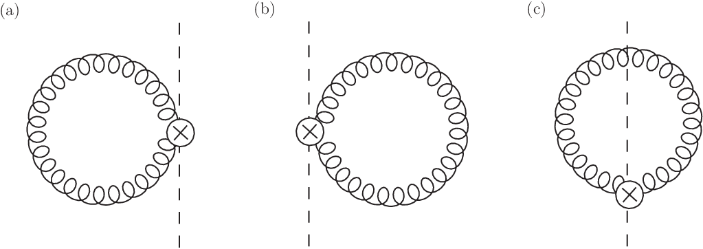
To determine the one-loop anomalous dimensions of $O_{S,P}$, we need to consider the Feynman diagrams in Fig. 1 as well as the wavefunction renormalization graphs. We regulate ultra-violet (UV) divergences using dimensional regularization and the infrared (IR) divergences by taking the external legs to be off-shell. It is then straightforward to extract the UV divergences and we find

$$Z_{S}=Z_{P}=1+\frac{\alpha_{s}}{4\pi}\frac{1}{\varepsilon_{\rm{UV}}}\Bigl[N_{c}\Bigl(\frac{2}{\varepsilon_{\rm{UV}}}+2\ln\frac{\mu^{2}}{m_{S}^{2}}+\frac{14}{3}+i\pi\Bigr)-\frac{2}{3}n_{f}\Bigr],$$

(39)

where $N_{c}$ and $n_{f}$ are the number of colors and flavors, respectively. From $Z_{S,P}$ we obtain the anomalous dimension for $O_{S}$ and $O_{P}$,

$$\gamma_{S,P}=\Bigl(\mu\frac{\partial}{\partial\mu}+\beta\frac{\partial}{\partial g}\Bigr)\ln Z_{S,P}=-\frac{\alpha_{s}}{\pi}\Bigl[N_{c}\Bigr(\ln\frac{\mu^{2}}{m_{S}^{2}}+\frac{7}{3}+i\frac{\pi}{2}\Bigr)-\frac{n_{f}}{3}\Bigr].$$

(40)

Note that

$\displaystyle\ln\frac{\mu^{2}}{m_{S}^{2}}+i\frac{\pi}{2}=\frac{1}{2}\ln\frac{\mu^{2}}{-m_{S}^{2}-i\epsilon}+\frac{1}{2}\ln\frac{\mu^{2}}{m_{S}^{2}}\,,$

(41)

so logarithms of both $+m_{S}^{2}$ and $-m_{S}^{2}$ appear. This is because there are corrections coming from soft exchanges between the two initial state particles, similar to Drell-Yan, which give rise to logs of $-m_{S}^{2}$, and soft exchanges between initial and final state particles, similar to deep inelastic scatttering, which give rise to logs of $+m_{S}^{2}$. From Eq. (40) we can infer the double logarithms in the $O(\alpha_{s})$ corrections to $C_{i}(\mu),~i=S,P$,

$\displaystyle C_{i}(\mu)=C_{i}^{(0)}\left[1-\frac{C_{A}\alpha_{s}}{4\pi}\left(\frac{1}{2}\log^{2}\left(\frac{-m_{S}^{2}-i\epsilon}{\mu^{2}}\right)+\frac{1}{2}\log^{2}\left(\frac{m_{S}^{2}}{\mu^{2}}\right)+...\right)\right]\,,$

(42)

where $...$ denotes terms without double logs. From this we see that if $\mu=m_{S}$, $C_{i}(m_{S})$ gets a $\pi^{2}$-enhanced contribution: $C_{i}(m_{S})=C_{i}^{(0)}(1+C_{A}\alpha_{s}(m_{S})\pi/8)$. For the range of $m_{S}$ considered in this paper, $\alpha_{s}(m_{S})\leq 0.1$. If $\alpha_{s}=0.1$, this $\pi^{2}$-enhanced correction increases the cross section by about 24%, and is half as big as the corresponding $\pi^{2}$-enhanced contribution to Higgs production. Refs. [3, 4] argued that the $\pi^{2}$-enhanced terms dominate the fixed-order corrections to Higgs production, and that these terms can be resummed to all orders by evolving the hard function from the scale $m_{H}^{2}$ to the scale $-m_{H}^{2}$. They also showed that the leading terms exponentiate. In our case, setting $\mu^{2}_{f}=-m_{S}^{2}$ does not remove the factor of $\pi^{2}$ in the hard coefficient. The double logs vanish if

$\displaystyle\mu^{2}=e^{\pi(\pm 1-i)/2}m_{S}^{2},$

(43)

but it is not clear that evolving to this complex scale will give a sensible resummation the $\pi^{2}$-enhanced contribution. Below we will calculate the $K$-factor with the next-to-leading order (NLO) $\pi^{2}$-enhanced correction. Even if the $\pi^{2}$-enhanced corrections exponentiate, the NLO correction should be a good approximation to the resummed result since $1+C_{A}\alpha_{s}\pi/4$ and $\exp(C_{A}\alpha_{S}\pi/4)$ differ by less than 3% for $\alpha_{s}=0.1$.

The soft functions in Eqs. (34) and (35) can be computed perturbatively when $\mu_{s}\sim m_{S}(1-z)\gg\Lambda_{\rm QCD}$. The Feynman diagrams in Fig. 2 give us the $O(\alpha_{s})$ corrections to $\bar{S}_{S}(m_{S}(1-z),\mu)$ and $\bar{S}_{P}(m_{S}(1-z),\mu)$:

	$\displaystyle\bar{S}_{S}^{(1)}(m_{S}(1-z),\mu)=\bar{S}_{P}^{(1)}(m_{S}(1-z),\mu)$		(44)
	$\displaystyle~~~=\frac{\alpha_{s}}{\pi}N_{c}\Biggl\{\delta(1-z)\Bigl[\frac{1}{\varepsilon_{\mathrm{UV}}^{2}}+\frac{1}{\varepsilon_{\mathrm{UV}}}\Bigl(\frac{1}{2}+\ln\frac{\mu^{2}}{m_{S}^{2}}\Bigr)+1-\frac{\pi^{2}}{4}+\frac{1}{2}\ln\frac{\mu^{2}}{m_{S}^{2}}+\frac{1}{2}\ln^{2}\frac{\mu^{2}}{m_{S}^{2}}\Bigr]$
	$\displaystyle~~~-\Bigl(\frac{2}{\varepsilon_{\mathrm{UV}}}+1+2\ln\frac{\mu^{2}}{m_{S}^{2}}\Bigr)\frac{1}{(1-z)_{+}}+4\Bigl(\frac{\ln(1-z)}{1-z}\Bigr)_{+}\Biggr\},$

where the plus distributions are defined in the standard way. Note that there is no IR divergence in the sum of the real and virtual diagrams in Fig. 2 [28]. The IR finiteness of the soft function can be easily understood in SCET because the soft function is just the Wilson coefficient obtained at the second-step matching.

References

- [1] A. Idilbi, X. d. Ji and F. Yuan, Nucl. Phys. B 753, 42 (2006) [arXiv:hep-ph/0605068].
- [2] T. Becher, M. Neubert and G. Xu, JHEP 0807, 030 (2008) [arXiv:0710.0680 [hep-ph]].
- [3] V. Ahrens, T. Becher, M. Neubert and L. L. Yang, arXiv:0809.4283 [hep-ph].
- [4] V. Ahrens, T. Becher, M. Neubert and L. L. Yang, arXiv:0808.3008 [hep-ph].
- [5] M. Kramer, E. Laenen and M. Spira, Nucl. Phys. B 511, 523 (1998) [arXiv:hep-ph/9611272].
- [6] S. Catani, D. de Florian, M. Grazzini and P. Nason, JHEP 0307, 028 (2003) [arXiv:hep-ph/0306211].
- [7] I. Dorsner and I. Mocioiu, Nucl. Phys. B 796, 123 (2008) [arXiv:0708.3332 [hep-ph]].
- [8] P. Fileviez Perez, H. Iminniyaz and G. Rodrigo, Phys. Rev. D 78, 015013 (2008) [arXiv:0803.4156 [hep-ph]].
- [9] P. Fileviez Perez, R. Gavin, T. McElmurry and F. Petriello, arXiv:0809.2106 [hep-ph].
- [10] T. Plehn and T. M. P. Tait, arXiv:0810.3919 [hep-ph].
- [11] S. Y. Choi, M. Drees, J. Kalinowski, J. M. Kim, E. Popenda and P. M. Zerwas, Phys. Lett. B 672, 246 (2009) [arXiv:0812.3586 [hep-ph]].
- [12] A. V. Povarov, P. Y. Popov and A. D. Smirnov, Phys. Atom. Nucl. 70, 739 (2007) [Yad. Fiz. 70, 771 (2007)].
- [13] P. Y. Popov, A. V. Povarov and A. D. Smirnov, Mod. Phys. Lett. A 20, 3003 (2005) [arXiv:hep-ph/0511149].
- [14] P. H. Frampton and S. L. Glashow, Phys. Rev. Lett. 58, 2168 (1987).
- [15] C. T. Hill, Phys. Lett. B 266, 419 (1991).
- [16] A. V. Manohar and M. B. Wise, Phys. Rev. D 74, 035009 (2006) [arXiv:hep-ph/0606172].
- [17] R. S. Chivukula and H. Georgi, Phys. Lett. B 188, 99 (1987).
- [18] G. D’Ambrosio, G. F. Giudice, G. Isidori and A. Strumia, Nucl. Phys. B 645, 155 (2002) [arXiv:hep-ph/0207036].
- [19] A. Kulesza and L. Motyka, arXiv:0807.2405 [hep-ph].
- [20] U. Langenfeld and S. O. Moch, arXiv:0901.0802 [hep-ph].
- [21] C. W. Bauer, S. Fleming and M. E. Luke, Phys. Rev. D 63, 014006 (2001) [arXiv:hep-ph/0005275]; C. W. Bauer, S. Fleming, D. Pirjol and I. W. Stewart, Phys. Rev. D 63, 114020 (2001) [arXiv:hep-ph/0011336].
- [22] C. W. Bauer, D. Pirjol and I. W. Stewart, Phys. Rev. D 65, 054022 (2002) [arXiv:hep-ph/0109045].
- [23] C. W. Bauer, S. Fleming, D. Pirjol, I. Z. Rothstein and I. W. Stewart, Phys. Rev. D 66, 014017 (2002) [arXiv:hep-ph/0202088].
- [24] M. I. Gresham and M. B. Wise, Phys. Rev. D 76, 075003 (2007) [arXiv:0706.0909 [hep-ph]].
- [25] M. Gerbush, T. J. Khoo, D. J. Phalen, A. Pierce and D. Tucker-Smith, Phys. Rev. D 77, 095003 (2008) [arXiv:0710.3133 [hep-ph]].
- [26] C. W. Bauer and I. W. Stewart, Phys. Lett. B 516, 134 (2001) [arXiv:hep-ph/0107001]; C. W. Bauer, D. Pirjol and I. W. Stewart, Phys. Rev. D 68, 034021 (2003) [arXiv:hep-ph/0303156].
- [27] J. Chay and C. Kim, Phys. Rev. D 65, 114016 (2002) [arXiv:hep-ph/0201197]; A. V. Manohar, T. Mehen, D. Pirjol and I. W. Stewart, Phys. Lett. B 539, 59 (2002) [arXiv:hep-ph/0204229].
- [28] T. Kinoshita, J. Math. Phys. 3 (1962) 650; T. D. Lee and M. Nauenberg, Phys. Rev. 133 (1964) B1549.
- [29] T. Becher and M. Neubert, Phys. Rev. Lett. 97, 082001 (2006) [arXiv:hep-ph/0605050].
- [30] T. Becher, M. Neubert and B. D. Pecjak, JHEP 0701, 076 (2007) [arXiv:hep-ph/0607228].
- [31] H. L. Lai et al. [CTEQ Collaboration], Eur. Phys. J. C 12, 375 (2000) [arXiv:hep-ph/9903282].
- [32] S. Fleming, A. H. Hoang, S. Mantry and I. W. Stewart, Phys. Rev. D 77, 074010 (2008) [arXiv:hep-ph/0703207].
- [33] G. P. Korchemsky and G. Marchesini, Nucl. Phys. B 406, 225 (1993) [arXiv:hep-ph/9210281].