Separatrix Map Analysis for Fractal Scatterings in Weak Interactions of Solitary Waves

The limit behaviors $\lim_{n\to\infty}\mathcal{F}^{n}(q_{0},m_{0})$ are important as they correspond to the outcomes of weak interactions. Indeed, from $m_{\infty}=\lim_{n\to\infty}m_{n}$ and the scaling relations (14), we can obtain the exit velocities $|\dot{\zeta}_{\infty}|$ from Eq. (10). For almost all initial points $(q_{0},m_{0})$, $m_{\infty}$ exists and is finite (while $q_{\infty}=\pm\infty$). Thus orbits of almost all initial points eventually escape to $q_{\infty}=\infty$ or $-\infty$ along the horizontal (constant-$m$) direction. But there are two special sets of initial points which are different. One set is the initial points which make $q_{n}=0$ for some $n\geq 0$, i.e.

For these points, iterations can not continue for $(q_{n+1},m_{n+1})$ since $q_{n}=0$, thus we call them singular points, and $\mathcal{S}$ the singular set. On these points, we formally let $m_{n+1}=\infty$, and consequently $m_{\infty}=\infty$ as well. For singular initial points, the exit velocities of weak interactions are infinite [see Eq. (10)], thus they correspond to peaks (of infinite height) in Fig. 1(c). The other set is the initial points $(q_{0},m_{0})$ which are periodic or quasi-periodic. On these points, $m_{n}$ oscillates forever, hence $m_{\infty}$ does not exist. These points correspond to spatially-localized and temporally oscillating bound states in the PDEs (1). In this case, we set $m_{\infty}=0$, which gives zero separation velocities $|\dot{\zeta}_{\infty}|$ from Eq. (10) (recall that $H<0$ for fractal scatterings [27]). This way, $m_{\infty}$ can be defined everywhere in the initial value plane $(q_{0},m_{0})$. Numerically we have computed $|m_{\infty}|$ over this plane (iterating 500 steps instead of infinite steps), and the result is plotted in Fig. 3 (here color levels correspond to $|m_{\infty}|$ values). This graph is a fractal, as can be easily verified by repeated zooms into it.

In Fig. 3, singular points form an infinite number of smooth curves. Each of these singular curves lies in the middle of a red stripe (of varying thickness), and all these singular curves form the backbone of the map’s fractal in Fig. 3. These singular curves are directly related to the singularity peaks (of infinite height) in the map’s exit-velocity fractals in Figs. 1(c) and 2(c). This is because on a singular curve, $m_{\infty}=\infty$, thus the corresponding exit velocity is also infinite [see Eq. (10)]. In view of this, these singular curves correspond to the singularity peaks in the ODE’s exit-velocity fractals and counterpart structures in the PDE’s exit-velocity fractals. These singularity peaks (or their counterparts) in turn form the backbones of the map’s, ODE’s and PDE’s exit-velocity fractals in Figs. 1 and 2. Thus if we can clearly characterize the singular curves of the map, then a good understanding of the fractals in the ODEs and PDEs will be reached. In the rest of this section, we focus on these singular curves. We will determine where they are located, how to identify them, what dynamics they represent, and what their asymptotics are at large or small values of $q_{0}$.

About these singular curves, each one is characterized by a unique finite binary sequence $\mathbf{a}=\mbox{sgn}(q_{0},q_{1},...,q_{n})$. Singular points on the same curve have the same binary sequence, while different singular curves have different sequences. Let us denote the singular curve with a binary sequence $\mathbf{a}=(a_{0},a_{1},...,a_{n})$ as $\gamma(\mathbf{a})$. Then

Here we allow $\mathbf{a}$ to be empty, in which case we get the simplest singular curve

which is the vertical axis. When $n=0$ (where $q_{1}=0$), we see from the map (3) that

These two curves are plotted in Fig. 4. They are located in the middle of the thickest red stripes in the right and left half planes of Fig. 3.

Now we determine the relations between singular curves with different binary sequences. From our definitions, we see that if $(q_{0},m_{0})\in\gamma(a_{0},\mathbf{a})$, then $\mathcal{F}(q_{0},m_{0})\in\gamma(\mathbf{a})$, where $\mathbf{a}$ is any finite binary sequence and $a_{0}=\pm 1$. In addition, if $a_{0}=1$, i.e. $q_{0}>0$, then $q_{1}-2m_{1}>0$ in view of Eq. (16), thus $\mathcal{F}(q_{0},m_{0})\in\Omega^{+}$. Similarly if $a_{0}=-1$, then $\mathcal{F}(q_{0},m_{0})\in\Omega^{-}$. As a result, we have

Or written differently, we have

These relations tell us that each singular curve $\gamma(\mathbf{a})$ has two pre-image singular curves $\gamma(1,\mathbf{a})$ and $\gamma(-1,\mathbf{a})$ under the map $\mathcal{F}$. In particular, $\gamma(1)$ and $\gamma(-1)$ are the two pre-image singular curves of $\gamma_{0}$.

Thus from the basic singular curve $\gamma_{0}$ given in Eq. (46), two singular curves $\gamma(1)$ and $\gamma(-1)$ in Eqs. (47)-(48) are obtained. We can successively construct $\gamma(\mathbf{a})$ for any finite binary sequence $\mathbf{a}$ by repeatedly applying the inverse map $\mathcal{F}^{-1}$ on $\gamma_{0}$. The first few of these singular curves are plotted in Fig. 4. It is easy to see from the map (3) that for any binary sequence $\mathbf{a}$, $\gamma(\mathbf{a})$ and $\gamma(-\mathbf{a})$ are anti-symmetric to each other about the origin, i.e.

thus we only consider curves on the right half plane with $\mathbf{a}=(1,a_{1},...,a_{n})$ below. From Fig. 4, we see that $\gamma(1)$, $\gamma(1,1)$, $\gamma(1,1,1)$, … form the primary cascading sequence from the left to the right. This sequence accumulates to the limit curve $\gamma(1,1,1,1,...)$ which is plotted as a dotted line in Fig. 4 and can be seen in Fig. 3. This primary sequence of singular curves defines the overall geometry of the map’s fractal in Fig. 3. On the left side of each primary curve, there is a secondary structure whose infinite curves are very close to each other and thus visually show as one “thick curve” in Fig. 4. Each secondary structure lies near its corresponding primary curve. To probe these secondary structures, we zoom into the box region of Fig. 4, which contains a segment of the secondary structure for the primary curve $\gamma(1)$. The result is shown in Fig. 5. From this zoomed-in graph, we see that among numerous curves in this secondary structure, there is a secondary sequence of curves $\gamma(1,-1)$, $\gamma(1,-1,-1)$, $\gamma(1,-1,-1,-1),\dots$ which cascades to the left. This secondary curve sequence defines the overall geometry of this secondary structure. Near each curve in this secondary sequence (and on its right hand side), there is a higher-order structure which can be probed by repeated zooms. Every time one zooms into a higher-order structure, the cascading direction of its higher-order sequence is reversed, and the side of the higher-order sequence relative to its associated curve (either left or right) is also reversed. The binary sequences for these higher-order-sequence curves are {$(\mathbf{a},1)$, $(\mathbf{a},1,1)$, $(\mathbf{a},1,1,1)$, …} when the sequence cascades to the right and lies on the right side of $\gamma(\mathbf{a})$, and {$(\mathbf{a},-1)$, $(\mathbf{a},-1,-1)$, $(\mathbf{a},-1,-1,-1)$ …} when the sequence cascades to the left and lies on the left side of $\gamma(\mathbf{a})$. Here $\mathbf{a}$ is the binary sequence for the associated curve of this higher-order sequence.

Based on the above pattern, we can identify any singular curve with an arbitrary binary sequence. For instance, to identify the curve with a binary sequence $\mathbf{a}=(1,1,-1,-1,-1,1,-1)$, we first go to the curve $\gamma(1)$ (see Fig. 4), find its associated primary sequence (which lies on its right hand side), and pick out the first member of that sequence (not counting $\gamma(1)$ itself). The picked curve is then $\gamma(1,1)$, see Fig. 4. Next, we go to the secondary curve sequence of $\gamma(1,1)$ (which lies on its left) and pick out the third member of that sequence, which is $\gamma(1,1,-1,-1,-1)$. Next we go to the higher-order sequence of $\gamma(1,1,-1,-1,-1)$ (which lies on its right) and pick out the first member of that sequence, which is $\gamma(1,1,-1,-1,-1,1)$. Lastly we go to the higher-order sequence of $\gamma(1,1,-1,-1,-1,1)$ (which lies on its left) and pick out the first member of that sequence, which will be the singular curve $\gamma(1,1,-1,-1,-1,1,-1)$ that we are looking for.

We have noted earlier in this section that the map $\mathcal{F}$ has a lot of periodic orbits. Then an interesting question is where these periodic orbits are located in the map’s fractal in Fig. 3, and how these orbits are related to the above singular curves. Clearly every periodic point can not lie on a singular curve $\gamma(\mathbf{a})$ with a finite binary sequence $\mathbf{a}$ in view of the definition (45) of $\gamma(\mathbf{a})$. But a periodic point can be viewed as being on a singular curve with an infinite binary sequence $\mathbf{a}$ whose digits are the signs of $q$ of the successive iteration points which repeat with the same period as the periodic point (here a singular curve with an infinite binary sequence can be defined as the limit of the singular curve with a finite binary sequence). Using this viewpoint, we can understand where periodic points should be located in the map’s fractal. For instance, in the period-two orbit {$(2^{-1/3},2^{-1/3})$, $(-2^{-1/3},-2^{-1/3})$}, the first point $(2^{-1/3},2^{-1/3})$ lies on the singular curve with the binary sequence $\mathbf{a}=(1,-1,1,-1,\dots)$, while the second point $(-2^{-1/3},-2^{-1/3})$ lies on the singular curve with the binary sequence $\mathbf{a}=(-1,1,-1,1,\dots)$. For another instance, in the period-four orbit {$(1,1),(1,0),(-1,-1),(-1,0)$}, the point $(1,1)$ lies on the singular curve with a binary sequence $(1,1,-1,-1,1,1,-1,-1,\dots)$, and the point $(1,0)$ lies on the singular curve with a binary sequence $(1,-1,-1,1,1,-1,-1,1,\dots)$, etc. The singular curves with these infinite binary sequences can be identified by the same scheme as we detailed above, thus we can ascertain where these periodic points are located in the map’s fractal. Obviously these infinite binary sequences of periodic points are infinitely close to their finite truncations, and points on the singular curves with truncated finite binary sequences have very different trajectories from those of the periodic points. Thus the periodic points of the map $\mathcal{F}$ are all unstable.

From the above singular-curve identification scheme, we see that all the singular curves on the right half of the $(q_{0},m_{0})$ plane lie between two special accumulation curves, $\gamma(1,1,1,1,....)$ and $\gamma(1,-1,-1,-1,-1,...)$ (see Figs. 4 and 5). So does the fractal of the map on the right half plane as well (see Fig. 3). In the whole plane, the map’s fractal lies between the two accumulation curves $\gamma(1,1,1,\dots)$ and $\gamma(-1,-1,-1,\dots)$.

Similar to the above tracking and identification of singular curves, we can also track how regions in the $(q,m)$ plane move under the map $\mathcal{F}$. This is helpful for us to see how the orbit of an initial point moves in the $(q,m)$ plane. Let us denote the regions above $\gamma(1,1,1,\dots)$ and below $\gamma(-1,-1,-1,\dots)$ as ${\cal D}_{0}$, and the region between $\gamma(1,-1,-1,-1,\dots)$ and $\gamma(-1,1,1,1,\dots)$ as ${\cal D}_{1}$. Then we find that

Other regions such as $\mathcal{F}^{-1}({\cal D}_{1})$ can be obtained with the help of singular curves whose pre-images under the inverse map $\mathcal{F}^{-1}$ have been detailed above (notice that the singular curve $\gamma_{0}$ lies in the middle of the region ${\cal D}_{1}$). Details will not be pursued in this paper.

Next we determine the asymptotic behaviors of singular curves as $q_{0}\to 0$ and $\pm\infty$. These asymptotic behaviors will be needed for our derivation of scaling laws of the exit-velocity fractals in the ODEs and PDEs as $\varepsilon\to 0$ under the unequal-amplitude initial conditions (19), see Sec. 4.2. But they will not be needed for scaling laws of fractals with equal-amplitude initial conditions (18), see Sec. 4.1. Since $\gamma(\mathbf{a})$ and $\gamma(-\mathbf{a})$ are anti-symmetric to each other, we only consider curves on the right half plane with $\mathbf{a}=(1,a_{1},...,a_{n})$ below.

The asymptotic behaviors of singular curves $\gamma(1,a_{1},...,a_{n})$ as $q_{0}\rightarrow 0^{+}$ and $+\infty$ can be obtained from $\gamma(1)$ in Eq. (47) and the recursion relations (51)-(52), and we get the following results:

1. 1.

   For any singular curve $\gamma(1,\mathbf{a})$, if $(q_{0},m_{0})\in\gamma(1,\mathbf{a})$, then

   $$m_{0}=q_{0}^{-2}+C_{\mathbf{a}}+...,\quad q_{0}\rightarrow 0^{+},$$

   (55)

   where $(2C_{\mathbf{a}},C_{\mathbf{a}})$ is the intersection point between $\gamma(\mathbf{a})$ and $\Omega$.

2. 2.

   If $(q_{0},m_{0})\in\gamma(1,a_{1},...,a_{n})$ with $a_{1}=...=a_{n}=1$ (i.e. on a primary singular curve), then

   $\displaystyle m_{0}=-\frac{1}{2(n+1)}q_{0}+D_{n}q_{0}^{-2}+...,\quad q_{0}\rightarrow+\infty,$

   (56)

   where

   $$D_{n}=1+\frac{n+1}{n}D_{n-1},\quad D_{0}=1.$$

   (57)

3. 3.

   If $(q_{0},m_{0})\in\gamma(1,a_{1},...,a_{n},-1,\mathbf{\hat{a}})$ where $a_{1}=...=a_{n}=1$ and $\mathbf{\hat{a}}$ is an arbitrary finite binary sequence, i.e. when $(q_{0},m_{0})$ lies in the secondary structure of a primary curve $\gamma(1,a_{1},...,a_{n})$, then

   	$\displaystyle m_{0}=$		$\displaystyle-\frac{1}{2(n+1)}q_{0}-\frac{1}{\sqrt{2(n+1)}}q_{0}^{-1/2}$		(58)
   		$\displaystyle+$	$\displaystyle\frac{(n+1)C_{\mathbf{\hat{a}}}}{\sqrt{2}}q_{0}^{-3/2}+...,\quad q_{0}\rightarrow+\infty.$

   where $(2C_{\mathbf{\hat{a}}},C_{\mathbf{\hat{a}}})$ is the intersection point between $\gamma(\mathbf{\hat{a}})$ and $\Omega$.

Notice from (56) and (58) that for any binary subsequence $\mathbf{\hat{a}}$, $\gamma(1,a_{1},..,a_{n},-1,\mathbf{\hat{a}})$ tends to $\gamma(1,a_{1},...,a_{n})$ as $q_{0}\to+\infty$, i.e. the distance between them goes to zero at large $q_{0}$ values. This explains why we could (and should) treat singular curves $\gamma(1,\mathbf{a},-1,\mathbf{\hat{a}})$ with arbitrary binary subsequences $\mathbf{\hat{a}}$ as the secondary structures associated with the primary curve $\gamma(1,\mathbf{a})$ earlier in this section.

To prove the first asymptotic result (55), let

Then using (16), we get

For $(q_{0},m_{0})\in\gamma(1,\mathbf{a})$, in view of the recursion relation (51), we see that $(q_{1},m_{1})\in\gamma(\mathbf{a})\bigcap\Omega^{+}$. When $q_{0}\to 0^{+}$, (59) shows that $q_{1}-2m_{1}\rightarrow 0^{+}$. Thus $(q_{1},m_{1})$ approaches the intersection point between $\gamma(\mathbf{a})$ and $\Omega$, i.e. $q_{1}\rightarrow 2C_{\mathbf{a}}$ and $m_{1}\rightarrow C_{\mathbf{a}}$. Substituting these asymptotic results into (60), (55) is then obtained.

The second and third asymptotic relations (56) and (58) can be proved by the induction method and by utilizing the recursion relation (51). These proofs are elementary and will be omitted.

In this subsection, we consider the first type of initial conditions (18) where the two solitary waves initially have equal amplitudes. In this case, the corresponding curve of the map’s initial points in the $(q_{0},m_{0})$ plane can be seen from (22) as

The reason for the restriction $\psi_{0}\in(-\pi/2,\pi/2)$ is that fractal scatterings can only arise in the $\psi_{0}$ intervals where $H<0$ [27]. In the present case, $H<0$ corresponds to the interval $\psi_{0}\in(-\pi/2,\pi/2)$. This parameterized curve $\lambda^{\varepsilon}$ is a straight line with slope one in the $(q_{0},m_{0})$ plane, see Fig. 6.

The map’s $|m_{\infty}|$ fractal in the initial-condition plane $(q_{0},m_{0})$ (see the previous section) is very instrumental for the understanding of exit-velocity fractals in the PDEs and ODEs. First of all, from the map’s $|m_{\infty}|$ fractal, together with the initial-value curve (61), the formula (10) and various scalings, we can easily construct the map’s exit-velocity fractal in Fig. 1(c). This exit-velocity fractal of the map can be readily understood. For instance, let us denote the $\psi_{0}$ value at the intersection of $\lambda^{\varepsilon}$ with a singular curve $\gamma(\mathbf{a})$ as $\psi^{\varepsilon}(\mathbf{a})$. At each $\psi^{\varepsilon}(\mathbf{a})$, the map’s exit-velocity graph has a singularity peak of infinite height. To illustrate, a few simple $\psi^{\varepsilon}(\mathbf{a})$ values are marked in Fig. 1(c). Using this connection, the map’s exit-velocity graph can be completely understood from the map’s $|m_{\infty}|$ fractal. Then the exit-velocity fractals in the ODEs and PDEs can be similarly understood. To be specific, we find that the primary window sequence in the exit-velocity fractals of Fig. 1, which cascades to the left with the first member being the widest window, are associated with the primary sequence of singular curves $\{\gamma(1),\gamma(1,1),\dots\}$ (at the intersection with the set $\lambda^{\varepsilon}$). The dense secondary structure on the right hand side of each primary window in the exit-velocity fractals of Fig. 1 corresponds to the secondary structure of each primary-sequence curve in the map’s $|m_{\infty}|$ fractal. In particular, the value $\psi^{\varepsilon}(1,-1)$, which is marked in Fig. 1(c), corresponds to the secondary singular curve $\gamma(1,-1)$ below the primary curve $\gamma(1)$ in Fig. 5. If we zoom into each secondary structure of a primary window in the exit-velocity fractals of Fig. 1, we will see secondary window sequences which cascade to the right, i.e. the cascading direction of secondary window sequences is reversed from that of the primary window sequence. The reason for this is that in the map’s $|m_{\infty}|$ fractal (see Fig. 4), the cascading direction of secondary sequences of singular curves is reversed from that of the primary sequence as we have explained before. The exit-velocity fractals of the PDE, the ODE and the map in Fig. 1 can be zoomed further, and all their microscopic structures can be inferred from the map’s singular curves in Fig. 4, or from the map’s $|m_{\infty}|$ fractal in Fig. 3 in general. One may notice that singularity peaks in the exit-velocity graphs appear only for the map and the ODEs, but not for the PDEs (see Fig. 1). Near such singularity peaks, the two solitary waves collide and coalesce, which makes our reduced ODE model (2) invalid. This explains the difference in those regions of the exit-velocity graphs between the ODEs and the PDEs.

From the map, we can obtain another important piece of information on the PDE/ODE’s fractal as the initial solitary-wave separation $\Delta\xi_{0}$ (i.e. $\zeta_{0}$) varies. In the present equal-amplitude initial conditions (18) and (20), if $\Delta\xi_{0}$ takes other (large) values, we can easily see from (61) that the values of $q_{0}=m_{0}$ are independent of $\Delta\xi_{0}$. This means that the exit-velocity fractal of the map [see Fig. 1(c)] will remain the same for different initial solitary-wave separations, which in turn implies the same for the exit-velocity fractals in the PDE/ODEs. This is a surprising fact, and it has been confirmed by our direct PDE/ODE simulations. It is noted that this fact does not hold for the unequal-amplitude initial conditions (19) because $(q_{0},m_{0})$ in such cases will depend on $\Delta\xi_{0}$, see (24).

In addition to the above qualitative understanding of the exit-velocity fractals in the PDEs and ODEs, we can further obtain the scaling properties of these fractals, i.e. we can determine quantitatively how the fractal structures in the PDEs and ODEs change as the parameter $\varepsilon$ varies. For this purpose, we notice that the map’s $|m_{\infty}|$ fractal at the intersection with $\lambda^{\varepsilon}$ on the right half plane lies between two accumulation points, $(q_{a},q_{a})=(0.741,0.741)$ and $(q_{b},q_{b})=(1.271,1.271)$ on $\gamma(1,-1,-1,-1,...)$ and $\gamma(1,1,1,1,...)$ respectively (see Fig. 6). In view of the initial-condition connection (61), the corresponding $\psi_{0}$ values of these two accumulation points are

These $\psi_{L}$ and $\psi_{R}$ values are the left and right boundaries of the map’s exit-velocity fractal on the negative $\Delta\phi_{0}$ axis [see Fig. 1(c)], and they are the map’s predictions for the fractal regions in the PDEs/ODEs. These formulae show that $\psi_{L,R}\rightarrow 0$ as $\varepsilon\rightarrow 0^{+}$, which means that the whole fractal region shrinks to $\psi_{0}=0$ as $\varepsilon\rightarrow 0^{+}$. Notice that when $\varepsilon=0$, the ODE solution $\zeta(\tau)$ under the equal-amplitude initial conditions (21) develops finite-time singularity at $\psi_{0}=0$, where $\mbox{Re}(C_{0})=0,\mbox{Im}(F_{0})=0$ (see Sec. 2). Thus when $\varepsilon\rightarrow 0^{+}$, the fractal region shrinks to the $\psi_{0}$ point which develops finite-time singularity in the integrable ODEs (see also [25]). Formulae (62) further show that this shrinking is at the rate of $\varepsilon^{1/3}$. To confirm this analytical prediction, we directly computed the exit-velocity fractals of the ODEs under the equal-amplitude initial conditions (21) as $\varepsilon$ takes on smaller and smaller values of 0.1, 0.01, 0.001 and 0.0001, and the results are displayed in Fig. 7. We see that as $\varepsilon\rightarrow 0^{+}$, the ODE’s fractal region indeed approaches $\psi_{0}=0$ [see Fig. 7(1-4)]. In addition, the fractal region’s left and right boundaries $\psi_{L}$ and $\psi_{R}$ indeed shrink in proportion to $\varepsilon^{1/3}$. Furthermore, the constants of proportion match the analytical values in Eq. (62) as well [see Fig. 7(5)]. Similar agreement has also been found for PDE fractals, see [26].

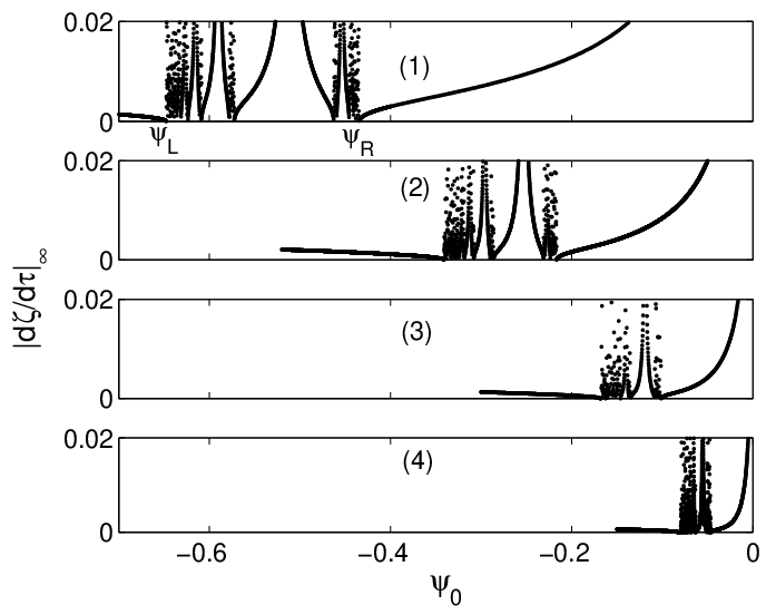
The comparison in Fig. 7(5) indicates that for the present equal-amplitude initial conditions, the map’s predictions are asymptotically accurate as $\varepsilon\to 0^{+}$. This is not surprising, as the fractal region here lies near $\psi_{0}=0$ when $|\varepsilon|\ll 1$. In this case, we can easily see from the definitions (8) and (9) that $E_{0}\ll 1$, $M_{0}\ll 1$ and $M_{0}/E_{0}\ll 1$ for the present initial conditions when $\psi_{0}$ lies inside the fractal region. Thus the assumptions for the derivation of the map (11)-(12) are satisfied, and consequently the map’s predictions are asymptotically accurate. For unequal-amplitude initial conditions (23), however, the assumption $M_{0}/E_{0}\ll 1$ will not be met in general, thus the map’s predictions will not be asymptotically accurate (even though they are still qualitatively accurate), see the next section for details.

Now we consider the second case of unequal-amplitude initial conditions (19). In this case, the corresponding curve of the map’s initial values in the $(q_{0},m_{0})$ plane can be seen from (24) as

where $T(\psi_{0})$ is defined in (25), $S(\psi_{0})$ given by (13), and the other involved parameters specified in (23). Here $H<0$ in the entire interval of $\psi_{0}\in[0,2\pi]$, thus no restriction on $\psi_{0}$ is needed [27]. These curves at two $\varepsilon$ values $\varepsilon_{1}=0.01$ and $\varepsilon_{2}=0.005$ are displayed in Fig. 8. Each $\lambda^{\varepsilon}$ is a closed curve, and it intersects a singular curve $\gamma(\mathbf{a})$ twice. Let us denote the $\psi_{0}$ values at the two intersections as $\psi^{\varepsilon}_{1}(\mathbf{a})$ and $\psi^{\varepsilon}_{2}(\mathbf{a})$, with $\psi^{\varepsilon}_{1}(\mathbf{a})<\psi^{\varepsilon}_{2}(\mathbf{a})$. These $\psi^{\varepsilon}_{1,2}(\mathbf{a})$ values are the singularity peaks of infinite height in the exit-velocity fractal of the map [see Fig. 2(c)]. On the singular curve $\gamma_{0}$, the intersection points would be denoted as $\psi^{\varepsilon}_{1}$ and $\psi^{\varepsilon}_{2}$. As $\varepsilon\to 0^{+}$, these intersections are such that $q_{0}\to+\infty$ in the right half plane and $q_{0}\to 0^{-}$ in the left half plane. This behavior can be readily understood by examining the intersections of $\lambda^{\varepsilon}$ with the horizontal and vertical axes. The intersections with the horizontal axis are such that $m_{0}=0$. In view of (63) as well as the expression (25) for $T(\psi_{0})$, we see that these intersections occur when $T(\psi_{0})=0$, i.e. when $\psi_{0}=0$ and $\pi$, regardless of the $\varepsilon$ values. Note that under the present initial conditions,

thus these two intersections on the horizontal axis are $(q_{A}\varepsilon^{-1/3},0)$ and $(q_{B}\varepsilon^{-1/3},0)$, which move to $(+\infty,0)$ as $\varepsilon\to 0^{+}$. Similarly, the intersections of $\lambda^{\varepsilon}$ with the vertical axis occur when $S(\psi_{0})=0$, i.e. when $\psi_{A}=1.988$ and $\psi_{B}=2.871$, regardless of the $\varepsilon$ values. Then the two intersection points on the vertical axis are $[0,T(\psi_{A})\varepsilon^{-1/3}]$ and $[0,T(\psi_{B})\varepsilon^{-1/3}]$, which approach $(0,-\infty)$ as $\varepsilon\to 0^{+}$.

References

- [1] M.J. Ablowitz and H. Segur, Solitons and the Inverse Scattering Transform, SIAM, Philadelphia, 1981.
- [2] A. Hasegawa and Y. Kodama, Solitons in Optical Communications, Clarendon, Oxford, 1995.
- [3] V. I. Karpman and V. V. Solov’ev, “A perturbation theory for soliton systems”, Physica D 3, 142-164 (1981).
- [4] V.S. Gerdjikov, D.J. Kaup, I.M. Uzunov and E.G. Evstatiev, “Asymptotic Behavior of N-Soliton Trains of the Nonlinear Schrödinger Equation”, Phys. Rev. Lett. 77, 3943 - 3946 (1996).
- [5] V. S. Gerdjikov, E. V. Doktorov and J. Yang, “Adiabatic Interaction of N-Ultrashort Solitons: Universality of the Complex Toda Chain Model.” Phys. Rev. E. 64, 056617 (2001).
- [6] J. Yang, “Suppression of Manakov-Soliton Interference in Optical Fibers”, Phys. Rev. E 65, 036606 (2002).
- [7] Y. Kodama, “On integrable systems with higher order corrections”, Phys. Lett. A 107, 245-249 (1985).
- [8] A. S. Fokas and Q.M. Liu, “Asymptotic Integrability of Water Waves”, Phys. Rev. Lett. 77, 2347 - 2351 (1996).
- [9] T.R. Marchant, “Asymptotic solitons for a higher-order modified Korteweg-de Vries equation”, Phys. Rev. E 66, 046623 (2002).
- [10] M.J. Ablowitz, M.D. Kruskal and J.F. Ladik, “Solitary Wave Collisions”, SIAM J. Appl. Math. 36, 428 (1979).
- [11] D. K. Campbell, J. S. Schonfeld, and C. A. Wingate, “Resonant structure in kink-antikink interactions in theory”, Physica D 9, 1-32 (1983).
- [12] P. Anninos, S. Oliveira, and R. A. Matzner, “Fractal structure in the scalar theory”, Phys. Rev. D 44, 1147-1160, 1991.
- [13] Y. S. Kivshar, Z. Fei, and L. Vázquez, “Resonant soliton-impurity interactions”, Phys. Rev. Lett. 67, 1177-1180, 1991.
- [14] J. Yang and Y. Tan, “Fractal structure in the collision of vector solitons”, Phys. Rev. Lett. 85, 3624-3627, 2000.
- [15] B.A. Malomed, Variational methods in nonlinear fiber optics and related fields, Progress in Optics Volume 43, North-Holland, 2002.
- [16] Z. Fei, Y. S. Kivshar, and L. Váquez, “Resonant kink-impurity interactions in the sine-Gordon model”, Phys. Rev. A 45, 6019-6030, 1992.
- [17] T. Ueda and W. L. Kath, “Dynamics of coupled solitons in nonlinear optical fibers”, Phys. Rev. A 42, 563 (1990).
- [18] Y. Tan and J. Yang, “Complexity and regularity of vector-soliton collisions”, Phys. Rev. E. 64, 056616 (2001).
- [19] R. H. Goodman and R. Haberman, “Interaction of sine-Gordon kinks with defects: The two-bounce resonance”, Phys. D. 195, pp. 303–323 (2004).
- [20] R. H. Goodman and R. Haberman, “Vector soliton interactions in birefringent optical fibers”, Phys. Rev. E 71, pp. 056605 (2005).
- [21] R. H. Goodman and R. Haberman, “Kink-antikink collisions in the phi-four equation: The n-bounce resonance and the separatrix map”, SIAM J. Appl. Dyn. Sys. 4, pp. 1195-1228 (2005).
- [22] R. H. Goodman and R. Haberman, “Chaotic Scattering and the n-Bounce Resonance in Solitary-Wave Interactions”, Phys. Rev. Lett. 98, 104103 (2007).
- [23] S.V. Dmitriev, Yu.S. Kivshar, and T. Shigenari, “Fractal structures and multiparticle effects in soliton scattering”, Phys. Rev. E 64, 056613, 2001.
- [24] S.V. Dmitriev and T. Shigenari, “Short-lived two-soliton bound states in weakly perturbed nonlinear Schrödinger equation”, Chaos 12, 324 (2002).
- [25] Y. Zhu and J. Yang, “Universal fractal structures in the weak interaction of solitary waves in generalized nonlinear Schrödinger equations”, Phys. Rev. E, 75 (2007), 036605.
- [26] Y. Zhu R. Haberman and J. Yang, “A universal map for fractal structures in weak solitary wave interactions”, Phys. Rev. Lett., 100, 143901 (2008).
- [27] Y. Zhu R. Haberman and J. Yang, “A Universal Separatrix Map for Weak Interactions of Solitary Waves in Generalized Nonlinear Schrödinger Equations”, Physica D 237, 2411(2008).
- [28] R. H. Goodman, “Chaotic scattering in solitary wave interactions: A singular iterated-map description”, Chaos, 18, 023113(2008)
- [29] D.K. Arrowsmith and C.M. Place, An introduction to Dynamical Systems, Cambridge University Press, Cambridge, 1990.