跳到论文正文
W Papers独立论文阅读器 arXiv:0903.3283 论文正文 计算阅读时间 · 0%
引用这篇论文根据当前论文元数据生成,正式投稿前建议核对。


License: arXiv.org perpetual non-exclusive license
arXiv:0903.3283v1 [math.CO] 19 Mar 2009

RNA-RNA interaction prediction:
partition function and base pair pairing probabilities

Fenix W.D. Huang1, Jing Qin1, Christian M. Reidys1,⋆ and Peter F. Stadler2 Address: 1Center for Combinatorics, LPMC-TJKLC
Nankai University
Tianjin 300071
P.R. China
Phone: *86-22-2350-6800
Fax: *86-22-2350-9272
2University of Leipzig
Leipzig D-04107
Härtelstr. 16-18
Germany
Email address: duck@santafe.edu
Date: March, 2009
Abstract.

In this paper, we study the interaction of an antisense RNA and its target mRNA, based on the model introduced by Alkan et al. (Alkan et al., J.  Comput.  Biol., Vol:267–282, 2006). Our main results are the derivation of the partition function [11] (Chitsaz et al., Bioinformatics, to appear, 2009), based on the concept of tight-structure and the computation of the base pairing probabilities. This paper contains the folding algorithm rip which computes the partition function as well as the base pairing probabilities in O⁡(N4​M2)+O⁡(N2​M4)O(N^{4}M^{2})+O(N^{2}M^{4}) time and O⁡(N2​M2)O(N^{2}M^{2}) space, where N,MN,M denote the lengths of the interacting sequences.

Key words and phrases: 
RNA-RNA interaction, joint structure, dynamic programming, partition function, base pairing probability, loop, RNA secondary structure.

1. Introduction

The discovery of small RNAs that bind to their target mRNAs in order to prohibit their translation and down-regulate the expression levels of corresponding genes has drawn a lot of attention in the RNA world [21]. Studies have shown that many RNA-RNA interactions play a significant role in different cellular processes, such as mediate pseudouridylation and methylation of rRNA [4], nucleotide insertion into mRNAs [6], splicing of pre-mRNA [35] and translation control or plasmid replication control [5, 12, 18].

Regulatory RNAs constitute a subclass of the antisense RNA family; encompassing the snRNAs, gRNAs and snoRNAs that play a role in the context of rRNA modification, RNA editing, mRNA spicing and plasmid copy-number regulation. In addition, antisense RNAs are synthesized for studying specific gene functions. Since the first published result on natural antisense RNAs which regulate gene expression in C. elegans [25, 34, 13, 27], Drosophila [24], and other organisms [31], the problem of predicting how two nucleic acid strands interact–the so called RNA-RNA interaction problem (RIP)–has come into focus.

As observed by Alkan et al. [2], the RIP is NP-complete. The actual argument constitutes an extension of the work of Akutsu [1] derived in the context of single RNA secondary structure prediction problems with pseudoknots. As in Rivas and Eddys pseudoknot folding algorithm [29] the general idea here is to consider specific classes of interactions, that can be computed via dynamic programming routines. There are several other methods that consider somewhat restricted versions of the RNA-RNA interaction. For instance, one method concatenates the two interacting sequences and subsequently employs a slightly modified standard secondary structure folding algorithm. The algorithms RNAcofold [14, 7], pairfold [3] and NUPACK [28] subscribe to this strategy. However, this approach cannot predict important motifs in RIPs, as for instance kissing hairpin loops. The concatenation idea has also been employed using the pseudoknot folding algorithm of Rivas and Eddy [29]. The resulting algorithm, however, does still not generate all relevant interaction structures [11, 26]. An alternative line of thought is to neglect all internal base-pairings in either strand and to compute the minimum free energy (mfe) secondary structure for their hybridization under this constraint. For instance, RNAduplex follows this line of thought making it formally equivalent to the classic secondary structure folding algorithm of Waterman [32, 15, 33, 30]. Furthermore we have the algorithm RNAup [23, 22] which uses the Alkan’s model, allowing for one interaction region having unbranched interactions within any loop. RNAup can therefore capture single but not multiple kissing hairpins. Finally there is IntaRNA [8] facilitating the efficient prediction of bacterial sRNA targets incorporating target site accessibility and seed regions.

Alkan et al. [2] derived a mfe algorithm for predicting the joint secondary structure of two interacting RNA molecules with polynomial time complexity. Here “joint structure”, see Fig. 1 for example, means that the intramolecular structures of each molecule are pseudoknot-free, the intermolecular binding pairs are noncrossing and there exist no so called “zig-zags” (see Section 1 for details). Zig-zags are sometimes referred to as tangles.

Refer to caption

Figure 1. Natural joint structure between small RNA molecules CopA(antisense) and CopT(target) in E.coli [2].

Recently, Chitsaz et.al. [11] presented a dynamic programming algorithm which computes the partition function in O⁡(N6)O(N^{6}) time. The key point for passing from the mfe folding of Alkan [2] to the partition function is a unique grammar by which each interaction structure can be generated. The dynamic programming routine for the partition function of RNA secondary structures is due to McCaskill [20] and can be outlined as follows: the free energy of a secondary structure is assumed additive in terms of its loops F⁡(S)=∑L∈SFLF(S)=\sum_{L\in S}F_{L}, where FLF_{L} denotes the free energy of a loop,LL. The additivity of the free energy translates itself into the multiplicativity in the contributions to the partition function QQ defined by Q=∑Se−F(S)/kTQ=\sum_{S}e^{-F(S)/kT}, where QQ is the sum over all the secondary structures SS of length MM. This factorization of terms can be realized by introducing Qb​(i,j)Q^{b}(i,j), where the sum is taken over all substructures S⁡[i,j]S[i,j] on the segment [i,j][i,j] for which (S⁡[i],S⁡[j])∈S⁡[i,j](S[i],S[j])\in S[i,j] and Qs​(i,j)Q^{s}(i,j) for all the configurations on [i,j][i,j], irrespective of whether or not i,ji,j are connected. In particular, we have Qs​(1,M)=QQ^{s}(1,M)=Q. Consequently, we arrive at the recursion, see Fig. 3

(1.1) Qs​(i,j)=1+∑h,ℓQs​(i,h−1)​Qb​(h,ℓ).Q^{s}(i,j)=1+\sum_{h,\ell}Q^{s}(i,h-1)Q^{b}(h,\ell).

Let us next recall the basic loops-types upon which the partition function and energy parameters [19] of RNA secondary structures are based:
(1) a hairpin-loop (𝖧𝖺⁡(i,j){\sf Ha}(i,j)), is a pair ((i,j),[i+1,j−1])((i,j),[i+1,j-1]), where (i,j)(i,j) is an arc and [i+1,j−1][i+1,j-1] is an interval, i.e. a sequence of consecutive vertices (i,i+1,…,j−1,j)(i,i+1,\dots,j-1,j), having energy parameter e−G𝖧𝖺(i,j)/kTe^{-G^{\sf Ha}(i,j)/kT}.
(2) an interior-loop (𝖨𝗇𝗍⁡(i1,j1,i2,j2){\sf Int}(i_{1},j_{1};i_{2},j_{2})), is a sequence ((i1,j1),[i1+1,i2−1],(i2,j2),[j2+1,j1−1])((i_{1},j_{1}),[i_{1}+1,i_{2}-1],(i_{2},j_{2}),[j_{2}+1,j_{1}-1]), where (i2,j2)(i_{2},j_{2}) is nested in (i1,j1)(i_{1},j_{1}) having the energy parameter e−G𝖨𝗇𝗍(i1,j1;i2,j2)/kTe^{-G^{\sf Int}(i_{1},j_{1};i_{2},j_{2})/kT}
(3) a multi-loop (𝖬⁡(i0,j0){\sf M}(i_{0},j_{0})), see Fig.2, is a sequence

(1.2) ([i0,i1−1],((i1,j1),[i1+1,j1−1]),…,((it,jt),[it+1,jt−1]),[jt+1,j0])([i_{0},i_{1}-1],((i_{1},j_{1}),[i_{1}+1,j_{1}-1]),\dots,((i_{t},j_{t}),[i_{t}+1,j_{t}-1]),[j_{t}+1,j_{0}])

having energy parameter e−(α1+α2(t+1)+α3c2)/kTe^{-(\alpha_{1}+\alpha_{2}(t+1)+\alpha_{3}c_{2})/kT}, where α1,α2,α3∈ℝ\alpha_{1},\alpha_{2},\alpha_{3}\in\mathbb{R}, tt is the number of R⁡[i0+1,j0−1]R[i_{0}+1,j_{0}-1]-maximal arcs inside R⁡[i0,j0]R[i_{0},j_{0}] and c2c_{2} is the number of isolated vertices contained in [i0,j0][i_{0},j_{0}].

Refer to caption

Figure 2. The standard loop-types for RNA secondary structures: hairpin-loop (top), interior-loop (middle) and multi-loop (bottom).

Based on the above loop-energies, we obtain the following recursion for Qb​(i,j)Q^{b}(i,j)

Qb​(i,j)\displaystyle Q^{b}(i,j) =e−G𝖧𝖺(i,j)/kT+∑k1,k2e−G𝖨𝗇𝗍(i,j,k1,k2)/kT\displaystyle=e^{-G^{\sf{Ha}}(i,j)/kT}+\sum_{k_{1},k_{2}}e^{-G^{\sf{Int}}(i,j,k_{1},k_{2})/kT}
+∑ℓQm​1(i+1,ℓ)Qm(ℓ+1,j−1)e−(α1+2α2)/kT,\displaystyle\qquad\qquad\qquad\;\quad+\sum_{\ell}Q^{m1}(i+1,\ell)Q^{m}(\ell+1,j-1)e^{-(\alpha_{1}+2\alpha_{2})/kT},

where

Qi,jm​1\displaystyle Q^{m1}_{i,j} =\displaystyle= ∑i≤ℓ<jQb(k,j)e−(α2+α3(ℓ−i))/kT\displaystyle\sum_{i\leq\ell<j}Q^{b}(k,j)e^{-(\alpha_{2}+\alpha_{3}(\ell-i))/kT}
Qm​(i,j)\displaystyle Q^{m}(i,j) =\displaystyle= ∑i≤ℓ<jQm​1(i,k)(Qm(ℓ+1,j)+e−α3(j−ℓ)/kT).\displaystyle\sum_{i\leq\ell<j}Q^{m1}(i,k)(Q^{m}(\ell+1,j)+e^{-\alpha_{3}(j-\ell)/kT}).

Refer to caption

Figure 3. The unique decomposition of secondary structures.

The key idea in this paper, which eventually leads to the derivation of both: the partition function as well as the base pairing probabilities, is the concept of a “tight structure”, introduced in Section 2. The tight structure plays a central role in our grammar and is the main tool for obtaining the base pairing probabilities. This paper includes the folding algorithm rip, which derives the partition function as well as the base pairing probabilities in O⁡(N4​M2)+O⁡(N2​M4)O(N^{4}M^{2})+O(N^{2}M^{4}) time and O⁡(N2​M2)O(N^{2}M^{2}) space. The source code of rip is available upon request.

2. Combinatorics of interaction structures

In this section we discuss some combinatorial properties of RNA interaction structures. The key idea introduced here is that of a tight structure. The main results of this section are:
∙\bullet there exist only four “types” of tight structures
∙\bullet given a joint structure J⁡(i,j,h,ℓ)J(i,j;h,\ell), each interaction bond (R⁡[i0],S⁡[j0])∈J⁡(i,j,h,ℓ)(R[i_{0}],S[j_{0}])\in J(i,j;h,\ell) is contained in a unique J⁡(i,j,h,ℓ)J(i,j;h,\ell)-tight structure
∙\bullet each joint structure uniquely decomposes into a sequence of tight structures and secondary structure segments
∙\bullet there exists a unique (but not canonical) decomposion of a tight structure.

Let us begin by making precise what we mean by interaction structures. Suppose we are given two diagrams [16, 17, 9, 10], RR and SS of length NN and MM, respectively. Let R⁡[i]R[i] and S⁡[i]S[i] denote the vertex ii of RR and SS, respectively. We shall assume that R⁡[1]R[1] denotes the 5′5^{\prime} end of RR and S⁡[1]S[1] denotes the 3′3^{\prime} end of SS as RNA sequences. The induced subgraph of SS with respect to the subsequence (S⁡[i],…,S⁡[j])(S[i],\dots,S[j]) is denoted by S⁡[i,j]S[i,j]. In particular, S⁡[i,i]=S⁡[i]S[i,i]=S[i] and S⁡[i,i−1]=∅S[i,i-1]=\varnothing. A complex C⁡(R,S,I)C(R,S,I) is a graph consisting of R,SR,S and a set of arcs of the form (R⁡[i],S⁡[j])(R[i],S[j]), II, see Fig. 4. We shall represent a complex CC by drawing RR on top of SS with the RR-arcs in the upper, the SS-arcs in the lower halfplane and II-arcs vertical. Given a complex CC, a subcomplex is the subgraph of CC, induced by R⁡[i1,j1]R[i_{1},j_{1}] and S⁡[i2,j2]S[i_{2},j_{2}].

Refer to caption

Figure 4. A complex CC induced by R⁡[1,14]R[1,14] and S⁡[1,13]S[1,13].

An arc is called interior if its start and endpoint are both contained in either RR or SS and exterior, otherwise. Let ≺1\prec_{1} be the partial order ≺1\prec_{1} over the set of interior arcs, given by

(2.1) (S[i1],S[j1])≺1(S[i2],S[j2])⟺i2<i1<j1<j2.(S[i_{1}],S[j_{1}])\prec_{1}(S[i_{2}],S[j_{2}])\quad\Longleftrightarrow\quad i_{2}<i_{1}<j_{1}<j_{2}.

Similarly, let ≺2\prec_{2} denote the partial order over the set of exterior arcs

(2.2) (S[i1],R[j1])≺2(S[i2],R[j2])⟺i1<i2,j1<j2.(S[i_{1}],R[j_{1}])\prec_{2}(S[i_{2}],R[j_{2}])\quad\Longleftrightarrow\quad i_{1}<i_{2},\ j_{1}<j_{2}.

Given an external arc, (R⁡[i],S⁡[j])(R[i],S[j]), an interior arc (R⁡[i1],R⁡[j1])(R[i_{1}],R[j_{1}]) is called its RR-ancestor if i1<i<j1i_{1}<i<j_{1} and (S⁡[i2],S⁡[j2])(S[i_{2}],S[j_{2}]) is the SS-ancestor of (R⁡[i],S⁡[j])(R[i],S[j]) if i2<j<j2i_{2}<j<j_{2}, respectively. We call (R⁡[i],S⁡[j])(R[i],S[j]) the descendant of (R⁡[i1],R⁡[j1])(R[i_{1}],R[j_{1}]) and (S⁡[i2],S⁡[j2])(S[i_{2}],S[j_{2}]) and the sets of RR-ancestors and SS-ancestors of (R⁡[i],S⁡[j])(R[i],S[j]) are denoted by AR​(R​[i],S​[j])A_{R}(R[i],S[j]) and AS​(R​[i],S​[j])A_{S}(R[i],S[j]). The ≺1\prec_{1}-minimal RR-ancestor and SS-ancestor of (R⁡[i],S⁡[j])(R[i],S[j]) are called its RR-parent and SS-parent, see Fig. 5. Finally, we call (R⁡[i1],R⁡[j1])(R[i_{1}],R[j_{1}]) and (S⁡[i2],S⁡[j2])(S[i_{2}],S[j_{2}]) dependent if they have a common descendant and independent, otherwise.

Refer to caption

Figure 5. Ancestors and parents: for the exterior arc (R⁡[3],S⁡[4])(R[3],S[4]), we have the following ancestor sets AR​(R⁡[3],S⁡[4])={(R⁡[1],R⁡[6]),(R⁡[2],R⁡[4])}A_{R}(R[3],S[4])=\{(R[1],R[6]),(R[2],R[4])\} and AS​(R⁡[3],S⁡[4])={(S⁡[2],S⁡[6]),(S⁡[3],S⁡[5])}A_{S}(R[3],S[4])=\{(S[2],S[6]),(S[3],S[5])\}. In particular, (R⁡[2],R⁡[4])(R[2],R[4]) and (S⁡[3],S⁡[5])(S[3],S[5]) are the RR-parent and SS-parent respectively.

Suppose C′=(R′,S′,I′)C^{\prime}=(R^{\prime},S^{\prime},I^{\prime}) is a subcomplex induced by R′=R⁡[i1,j1]R^{\prime}=R[i_{1},j_{1}] and S′=S⁡[i2,j2]S^{\prime}=S[i_{2},j_{2}] and suppose furthermore there exists an exterior arc, (R⁡[a],S⁡[b])(R[a],S[b]), with ancestors (R⁡[i],R⁡[j])(R[i],R[j]) and (S⁡[i′],S⁡[j′])(S[i^{\prime}],S[j^{\prime}]). The arc (R⁡[i],R⁡[j])(R[i],R[j]) is C′C^{\prime}-subsumed in (S⁡[i′],S⁡[j′])(S[i^{\prime}],S[j^{\prime}]), if for any (R⁡[k],S⁡[k′])∈I′(R[k],S[k^{\prime}])\in I^{\prime} with i<k<ji<k<j, there exists some k′k^{\prime} such that i′<k′<j′i^{\prime}<k^{\prime}<j^{\prime}. In case of C′=CC^{\prime}=C, we call (R⁡[i],R⁡[j])(R[i],R[j]) simply “subsumed” in (S⁡[i′],S⁡[j′])(S[i^{\prime}],S[j^{\prime}]), see Fig. 6. If (R⁡[i1],R⁡[j1])(R[i_{1}],R[j_{1}]) is subsumed in (S⁡[i2],S⁡[j2])(S[i_{2}],S[j_{2}]) and vice versa, we call these arcs equivalent.

Refer to caption

Figure 6. Subsumed and equivalent arcs: (R⁡[1],R⁡[8])(R[1],R[8]) subsumes (S⁡[1],S⁡[4])(S[1],S[4]) and (S⁡[5],S⁡[8])(S[5],S[8]). Furthermore, (R⁡[2],R⁡[5])(R[2],R[5]) is equivalent to (S⁡[1],S⁡[4])(S[1],S[4]).

A joint structure, J⁡(R⁡[i,j],S⁡[h,ℓ],I′)=J⁡(i,j,h,ℓ)J(R[i,j];S[h,\ell],I^{\prime})=J(i,j;h,\ell) is a subcomplex of C⁡(R,S,I)C(R,S,I) with the following properties, see Fig. 7:
∙\bullet RR, SS are secondary structures
∙\bullet there exist no external pseudoknots, i.e. if (R⁡[i1],S⁡[j1]),(R⁡[i2],S⁡[j2])∈I′(R[i_{1}],S[j_{1}]),(R[i_{2}],S[j_{2}])\in I^{\prime} where i1<i2i_{1}<i_{2}, then j1<j2j_{1}<j_{2}.
∙\bullet there exist no “zig-zags”, see Fig.8. I.e. if (R⁡[i1],R⁡[j1])(R[i_{1}],R[j_{1}]) and (S⁡[i2],S⁡[j2])(S[i_{2}],S[j_{2}]) are dependent, then either (R⁡[i1],R⁡[j1])(R[i_{1}],R[j_{1}]) is subsumed by (S⁡[i2],S⁡[j2])(S[i_{2}],S[j_{2}]) or vice versa.

Refer to caption

Figure 7. A joint structure induced by R⁡[1,24]R[1,24] and S⁡[1,23]S[1,23].

In absence of exterior arcs we refer to a joint structure as a secondary structure segment, or segment for short. We call S⁡[i1,j1]S[i_{1},j_{1}] maximal if there exists no segment, S⁡[i,j]S[i,j], containing S⁡[i1,j1]S[i_{1},j_{1}]. We remark that the idea of a joint structure goes back to [2] and has also been utilized in [11]. One key idea in our approach is to introduce a specific joint structure, called a tight, which is in some sense a generalization of the loop. It can be viewed as the transitive closure of a loop with respect to exterior arcs.

Refer to caption

Figure 8. A zig-zag, generated by (R⁡[2],S⁡[1])(R[2],S[1]), (R⁡[3],S⁡[3])(R[3],S[3]) and (R⁡[5],S⁡[4])(R[5],S[4]).

Let J⁡(a,b,c,d)J(a,b;c,d) be a fixed joint structure. A joint structure, J⁡(i,j,h,ℓ)⊂J⁡(a,b,c,d)J(i,j;h,\ell)\subset J(a,b;c,d) is J⁡(a,b,c,d)J(a,b;c,d)-tight (or tight in J⁡(a,b,c,d)J(a,b;c,d)) if:
∙\bullet there exists at least one exterior arc (R⁡[i1],S⁡[j1])(R[i_{1}],S[j_{1}])
∙\bullet for any (R⁡[i1],S⁡[j1])(R[i_{1}],S[j_{1}]), we have

(2.3) (AR​(R⁡[i1],S⁡[j1])∪AS​(R⁡[i1],S⁡[j1]))∩J⁡(a,b,c,d)∈J⁡(i,j,h,ℓ)(A_{R}(R[i_{1}],S[j_{1}])\cup A_{S}(R[i_{1}],S[j_{1}]))\cap J(a,b;c,d)\in J(i,j;h,\ell)

∙\bullet J⁡(i,j,h,ℓ)J(i,j;h,\ell) is minimal with respect to ⊂\subset.

Given a tight (tjs), J⁡(i,j,h,ℓ)J(i,j;h,\ell), we observe that neither one of the vertices i,j,hi,j,h and ℓ\ell, are start or endpoint of a segment. In particular, i,j,hi,j,h and ℓ\ell are not isolated. In combination with the non zig-zag property, we observe that there are only the following four types of tights (▽)(\bigtriangledown), (△)(\triangle), (□)(\square) or (∘)(\circ), see Fig.9:
(▽)(\bigtriangledown): (R⁡[i],R⁡[j])∈J⁡(i,j,h,ℓ)(R[i],R[j])\in J(i,j;h,\ell) and (S⁡[h],S⁡[ℓ])∉J⁡(i,j,h,ℓ)(S[h],S[\ell])\not\in J(i,j;h,\ell)
(△)(\bigtriangleup): (S⁡[h],S⁡[ℓ])∈J⁡(i,j,h,ℓ)(S[h],S[\ell])\in J(i,j;h,\ell) and (R⁡[i],R⁡[j])∉J⁡(i,j,h,ℓ)(R[i],R[j])\not\in J(i,j;h,\ell)
(□)(\square): {(R⁡[i],R⁡[j]),(S⁡[h],S⁡[ℓ])}∈J⁡(i,j,h,ℓ)\{(R[i],R[j]),(S[h],S[\ell])\}\in J(i,j;h,\ell)
(∘)(\circ): {(R⁡[i],S⁡[h])}=J⁡(i,j,h,ℓ)\{(R[i],S[h])\}=J(i,j;h,\ell) and i=ji=j, h=ℓh=\ell, i.e. we have a single interaction.
Let JA​(i,j,h,ℓ)J_{A}(i,j;h,\ell) denote a tight structure J⁡(i,j,h,ℓ)J(i,j;h,\ell) having type ξ\xi, where ξ∈A⊂{▽,△,□,∘}\xi\in A\subset\{\bigtriangledown,\bigtriangleup,\square,\circ\}. In particular, Jξ​(i,j,h,ℓ)J_{\xi}(i,j;h,\ell) is a tight structure J⁡(i,j,h,ℓ)J(i,j;h,\ell) of type ξ\xi.

Refer to caption

Figure 9. From left to right: (tjs) of type (▽)(\bigtriangledown), (△)(\triangle), (□)(\square) and (∘)(\circ).
Proposition 2.1.

Let J⁡(a,b,c,d)J(a,b,c,d) be a joint structure, then the following assertions hold:
(a) if J⁡(i,j,h,ℓ)J(i,j;h,\ell) is tight in J⁡(a,b,c,d)J(a,b,c,d), then J⁡(i,j,h,ℓ)J(i,j;h,\ell) has type τ∈{▽,△,□,∘}\tau\in\{\bigtriangledown,\triangle,\square,\circ\}
(b) any exterior arc is contained in a unique J⁡(a,b,c,d)J(a,b,c,d)-(tjs)
(c) J⁡(a,b,c,d)J(a,b,c,d) decomposes into a unique sequence of (tjs) and maximal segments.

Suppose we are given two exterior arcs (R⁡[i1],S⁡[j1]),(R⁡[i2],S⁡[j2])∈J⁡(i,j,h,ℓ)(R[i_{1}],S[j_{1}]),(R[i_{2}],S[j_{2}])\in J(i,j;h,\ell). For two J⁡(i,j,h,ℓ)J(i,j;h,\ell)-tight structures, JT​((R⁡[i1],S⁡[j1]))J_{T}((R[i_{1}],S[j_{1}])), JT​((R⁡[i2],S⁡[j2]))J_{T}((R[i_{2}],S[j_{2}])) we set

JT((R[i1],S[j1]))=JT((R[i2],S[j2]))⟺(R[i1],S[j1])1∼J⁡(i,j,h,ℓ)(R[i2],S[j2]).J_{T}((R[i_{1}],S[j_{1}]))=J_{T}((R[i_{2}],S[j_{2}]))\quad\Longleftrightarrow\quad(R[i_{1}],S[j_{1}])_{1}\sim_{J(i,j;h,\ell)}(R[i_{2}],S[j_{2}]).

Suppose JT​(i,j,r,s)J_{T}(i,j;r,s) is a tight structure where i≤a<b≤ji\leq a<b\leq j and r≤c<d≤sr\leq c<d\leq s. A double-tight structure JD​T​(i,j,r,s)J_{DT}(i,j;r,s) in JT​(i,j,r,s)J_{T}(i,j;r,s), is a joint structure J⁡(i,j,r,s)J(i,j;r,s) such that J⁡(i,j,r,s)⊂JT​(i,j,r,s)J(i,j;r,s)\subset J_{T}(i,j;r,s) and

(2.4) JD​T​(i,j,r,s)=(JT​(i,a,r,c),J⁡(a+1,b−1,c+1,d−1),JT​(b,j,d,s))J_{DT}(i,j;r,s)=(J_{T}(i,a;r,c),J(a+1,b-1;c+1,d-1),J_{T}(b,j;d,s))

where JT​(i,a,r,c)J_{T}(i,a;r,c) and JT​(b,j,d,s)J_{T}(b,j;d,s) are J⁡(a+1,b−1,c+1,d−1)J(a+1,b-1;c+1,d-1)-tight structures, see Fig. 10.

Refer to caption

Figure 10. A double-tight structure JD​T​(6,15,1,11)J_{DT}(6,15;1,11) in J⁡(2,15,1,11)J(2,15;1,11). Note that the joint structure J⁡(1,15,1,11)J(1,15;1,11) itself is a ▽\bigtriangledown-tight.

Refer to caption

Figure 11. Decomposing tights: we show how to decompose a tights of the types (▽)(\bigtriangledown), (△)(\triangle) or (□)(\square) via to Corollary 2.2, Corollary 2.3 and Corollary 2.4.
Corollary 2.2.

Let J▽​(i,j,r,s)J_{\bigtriangledown}(i,j;r,s) be a tight structure of type ▽\bigtriangledown and let ζ1=(R⁡[h1],S⁡[ℓ1])\zeta_{1}=(R[h_{1}],S[\ell_{1}]) and ζ2=(R⁡[h2],S⁡[ℓ2])\zeta_{2}=(R[h_{2}],S[\ell_{2}]) be the minimal and maximal exterior arcs in J⁡(i,j,r,s)J(i,j;r,s) and i+1≤i1≤j1≤j−1i+1\leq i_{1}\leq j_{1}\leq j-1. Then

(2.5) J⁡(i+1,j−1,r,s)={(R⁡[i+1,i1−1],J{▽,∘}​(i1,j1,r,s),R⁡[j1+1,j−1]),ifζ1∼J⁡(i+1,j−1,r,s)ζ2(R⁡[i+1,i1−1],JD​T​(i1,j1,r,s),R⁡[j1+1,j−1])otherwise,\begin{split}J(i+1,j-1;r,s)=\ \ \ \ \ \ \ \ \ \ \ \ \ \ \ \ \ \ \ \ \ \ \ \ \ \ \ \ \ \ \ \ \ \ \ \ \ \ \ \ \ \ \ \ \ \ \ \ \ \ \ \ \ \ \ \ \ \ \ \ \ \ \ \ \ \ \ \ \ \ \ \ \ \ \ \ \ \ \ \ \ \ \ \ \ \ \ \ \ \ \ \\ \begin{cases}(R[i+1,i_{1}-1],J_{\{\bigtriangledown,\circ\}}(i_{1},j_{1};r,s),R[j_{1}+1,j-1]),\ &\text{\rm if}\ \zeta_{1}\sim_{J(i+1,j-1;r,s)}\zeta_{2}\\ (R[i+1,i_{1}-1],J_{DT}(i_{1},j_{1};r,s),R[j_{1}+1,j-1])&\text{\rm otherwise,}\end{cases}\end{split}

where J{▽,∘}​(i1,j1,r,s)J_{\{\bigtriangledown,\circ\}}(i_{1},j_{1};r,s) denotes a J⁡(i+1,j−1,r,s)J(i+1,j-1;r,s)-tight of type △\triangle or ∘\circ.

Of course we have

Corollary 2.3.

Let J△​(i,j,r,s)J_{\triangle}(i,j;r,s) be a tight structure of type △\triangle and let ζ1=(R⁡[h1],S⁡[ℓ1])\zeta_{1}=(R[h_{1}],S[\ell_{1}]) and ζ2=(R⁡[h2],S⁡[ℓ2])\zeta_{2}=(R[h_{2}],S[\ell_{2}]) be the minimal and maximal exterior arcs in J⁡(i,j,r,s)J(i,j;r,s) and r+1≤r1≤s1≤s−1r+1\leq r_{1}\leq s_{1}\leq s-1. Then

(2.6) J⁡(i,j,r+1,s−1)={(S⁡[r+1,r1−1],J{△,∘}​(i,j,r1,s1),S⁡[s1+1,s−1]),ifζ1∼J⁡(i,j,r+1,s−1)ζ2(S⁡[r+1,r1−1],JD​T​(i,j,r1,s1),S⁡[s1+1,s−1]),otherwise,\begin{split}J(i,j;r+1,s-1)=\ \ \ \ \ \ \ \ \ \ \ \ \ \ \ \ \ \ \ \ \ \ \ \ \ \ \ \ \ \ \ \ \ \ \ \ \ \ \ \ \ \ \ \ \ \ \ \ \ \ \ \ \ \ \ \ \ \ \ \ \ \ \ \ \ \ \ \ \ \ \ \ \ \ \ \ \ \ \ \ \ \ \ \ \ \ \ \ \ \ \ \\ \begin{cases}(S[r+1,r_{1}-1],J_{\{\triangle,\circ\}}(i,j;r_{1},s_{1}),S[s_{1}+1,s-1]),\ &\text{\rm if}\ \zeta_{1}\sim_{J(i,j;r+1,s-1)}\zeta_{2}\\ (S[r+1,r_{1}-1],J_{DT}(i,j;r_{1},s_{1}),S[s_{1}+1,s-1]),&\text{\rm otherwise,}\end{cases}\end{split}

where J{△,∘}​(i1,j1,r,s)J_{\{\triangle,\circ\}}(i_{1},j_{1};r,s) denotes a J⁡(i,j,r+1,s−1)J(i,j;r+1,s-1)-tight of type △\bigtriangleup or ∘\circ.

Corollary 2.4.

Let J⁡(i,j,r,s)J(i,j;r,s) be a tight structure of type □\square and set i+1≤i1≤j1≤j−1i+1\leq i_{1}\leq j_{1}\leq j-1, then Jt​(i,j,r,s)J_{t}(i,j;r,s) decomposes as follows:

(2.7) J⁡(i+1,j−1,r,s)=(R⁡[i+1,i1−1],J{△,□}​(i1,j1,r,s),R⁡[j1+1,j−1]),J(i+1,j-1;r,s)=(R[i+1,i_{1}-1],J_{\{\triangle,\square\}}(i_{1},j_{1};r,s),R[j_{1}+1,j-1]),

where J{△,□}​(i1,j1,r,s)J_{\{\triangle,\square\}}(i_{1},j_{1};r,s) denotes a J⁡(i+1,j−1,r,s)J(i+1,j-1;r,s)-tight of type △\triangle or □\square.

2.1. Proofs

Proof of Proposition 2.1

Proof.

Let (R⁡[i],S⁡[j])(R[i],S[j]) be the maximal (rightmost) exterior arc of J⁡(a,b,c,d)J(a,b,c,d). We consider the set of maximal (R⁡[i],S⁡[j])(R[i],S[j])-ancestors, MM. In case of M=∅M=\varnothing we immediately observe J⁡(i,j,h,ℓ)=(R⁡[i],S⁡[j])J(i,j;h,\ell)=(R[i],S[j]), i.e.  J⁡(i,j,h,ℓ)J(i,j;h,\ell) is of type ∘\circ. Suppose next |M|=1|M|=1. By symmetry we can, without loss of generality, assume M={(R⁡[i1],R⁡[j1])}M=\{(R[i_{1}],R[j_{1}])\}. Let (R⁡[i0],S⁡[j0])(R[i_{0}],S[j_{0}]) the minimal exterior arc being an descendant of (R⁡[i1],R⁡[j1])(R[i_{1}],R[j_{1}]) and let j0∗j_{0}^{*} denote either the startpoint of the maximal (R⁡[i0],S⁡[j0])(R[i_{0}],S[j_{0}]) SS-ancestor or set j0∗=j0j_{0}^{*}=j_{0} if no such ancestor exists. Then, by construction, J⁡(i1,j1,j0∗,j)J(i_{1},j_{1};j_{0}^{*},j) is tight in J⁡(a,b,c,d)J(a,b,c,d). Finally, in case of |M|=2|M|=2, i.e. M={(R⁡[i1],R⁡[j1]),(S⁡[r1],S⁡[s1])}M=\{(R[i_{1}],R[j_{1}]),(S[r_{1}],S[s_{1}])\}. We may, without loss of generality, assume that (R⁡[i1],R⁡[j1])(R[i_{1}],R[j_{1}]) subsumes (S⁡[r1],S⁡[s1])(S[r_{1}],S[s_{1}]). Again we consider the minimal descendant of (R⁡[i1],R⁡[j1])(R[i_{1}],R[j_{1}]), (R⁡[z],S⁡[x])(R[z],S[x]). Let x∗x^{*} be either the startpoint of the maximal SS-ancestor of (R⁡[z],S⁡[x])(R[z],S[x]) or x∗=xx^{*}=x, otherwise. Then J⁡(i1,j1,x∗,s1)J(i_{1},j_{1};x^{*},s_{1}) is tight. If (R⁡[i1],R⁡[j1])(R[i_{1}],R[j_{1}]) is equivalent to OPENS⁡[r1],S⁡[s1])S[r_{1}],S[s_{1}]), then J⁡(i1,j1,r1,s1)J(i_{1},j_{1};r_{1},s_{1}) is tight. In the above procedure we have constructed a (tjs), J∗J^{*}, of type τ∈{▽,△,□,∘}\tau\in\{\bigtriangledown,\triangle,\square,\circ\} that contains the maximal exterior J⁡(a,b,c,d)J(a,b,c,d)-arc. By definition of tight and the fact that we have noncrossing arcs it follows that any other (tjs) of J⁡(a,b,c,d)J(a,b,c,d) is disjoint to J∗J^{*}. We proceed by considering the rightmost exterior arc of J⁡(a,b,c,d)J(a,b,c,d) that is not contained in J∗J^{*}, concluding assertion (c) by induction on the number of exterior arcs of J⁡(a,b,c,d)J(a,b,c,d). Since any exterior arc of J⁡(a,b,c,d)J(a,b,c,d) is contained in a unique (tjs) generated by the above procedure, (b) follows, see Fig. 12. ∎

Refer to caption

Figure 12. Illustration of Prop.2.1.

Proof to Corollary 2.2

Proof.

According to Prop. 2.1(b), there exist unique J⁡(i+1,j−1,r,s)J(i+1,j-1;r,s)-tight structures J⁡(i1,i2,r,r1)J(i_{1},i_{2};r,r_{1}) and J⁡(j2,j1,s1,s)J(j_{2},j_{1};s_{1},s) such that J⁡(i1,i2,r,r1)=JT​(ζ1)J(i_{1},i_{2};r,r_{1})=J_{T}(\zeta_{1}) and J⁡(j2,j1,s1,s)=JT​(ζ2)J(j_{2},j_{1};s_{1},s)=J_{T}(\zeta_{2}), respectively. We have the following two scenarios: in case of ζ1∼J⁡(i+1,j−1,r,s)ζ2\zeta_{1}\sim_{J(i+1,j-1;r,s)}\zeta_{2}, i.e.  JT​(ζ1)=JT​(ζ2)J_{T}(\zeta_{1})=J_{T}(\zeta_{2}), we have either r=sr=s, in which case J⁡(i1,j1,r,s)J(i_{1},j_{1};r,s) is of type ∘\circ and in view of (S⁡[r],S⁡[s])∉J▽​(i,j,r,s)(S[r],S[s])\not\in J_{\bigtriangledown}(i,j;r,s) J⁡(i1,j1,r,s)J(i_{1},j_{1};r,s) is of type ▽\bigtriangledown, otherwise. In case of ζ1≁J⁡(i+1,j−1,r,s)ζ2\zeta_{1}\not\sim_{J(i+1,j-1;r,s)}\zeta_{2}, J⁡(i1,j1,r,s)J(i_{1},j_{1};r,s) is a J⁡(i+1,j−1,r,s)J(i+1,j-1;r,s)-double tight structure. ∎

Proof of Corollary 2.4

Proof.

We observe that there exist only one J⁡(i+1,j−1,r,s)J(i+1,j-1;r,s)-tight structure, since (S⁡[r],S⁡[s])∈J⁡(i+1,j−1,r,s)(S[r],S[s])\in J(i+1,j-1;r,s). We consider the set MM, consisting of arcs that are equivalent to (S⁡[r],S⁡[s])(S[r],S[s]). According to Prop. 2.1, (c), we have

J⁡(i+1,j−1,r,s)={(R⁡[i+1,i1−1],J△​(i1,j1,r,s),R⁡[j1+1,j−1])for​M=∅(R⁡[i+1,i1−1],J□​(i1,j1,r,s),R⁡[j1+1,j−1])otherwise.J(i+1,j-1;r,s)=\begin{cases}(R[i+1,i_{1}-1],J_{\triangle}(i_{1},j_{1};r,s),R[j_{1}+1,j-1])&\text{\rm for}M=\varnothing\\ (R[i+1,i_{1}-1],J_{\square}(i_{1},j_{1};r,s),R[j_{1}+1,j-1])&\text{\rm otherwise.}\end{cases}

∎

3. Unique decomposition

We showed in Section 2 via Prop. 2.1 that an arbitrary joint structure uniquely decomposes into a sequence of segments and tight structures. Via the combinatorial corollaries, Cor. 2.2, Cor. 2.3 and Cor. 2.4 we introduced a unique decomposition procedure for tights, see Fig. 13 and Fig. 14, below.

Refer to caption

Figure 13. Illustration of Cor. 2.2.

Refer to caption

Figure 14. Illustration of Cor. 2.4.

In this section we give the algorithmic interpretation of the above results. In the course of our analysis we derive for any joint structure J⁡(1,N,1,M)J(1,N;1,M) a unique decomposition tree via Procedure (a), (b) and (c), below, see Fig. 15.

Refer to caption

Figure 15. Illustration of Procedure (a), Procedure (b) and Procedure (c) for the joint structure J⁡(1,12,1,8)J(1,12,1,8). From left to right we display Ta​(1,12,1,8)T_{a}(1,12;1,8), Tb​(5,6,6,9)T_{b}(5,6;6,9) and Tc​(R​[7,12])T_{c}(R[7,12]).

Let us begin by giving an interpretation of Prop. 2.1.
Procedure (a):
input: a joint structure ϑ0=J⁡(i,j,h,ℓ)\vartheta_{0}=J(i,j;h,\ell), which is not ϑ0\vartheta_{0}-tight or a ms
output: a unique tree Ta​(ϑ0)=(Va​(T),Ea​(T))T_{a}(\vartheta_{0})=(V_{a}(T),E_{a}(T))
Let i≤j∗≤j+1i\leq j^{*}\leq j+1 and R⁡[j∗,j]R[j^{*},j] be the ϑ0\vartheta_{0}-ms contain jj. In particular, j∗=j+1j^{*}=j+1 in case of such an ms does not exist and j∗=1j^{*}=1 if R⁡[i,j]R[i,j] itself is a ms. Analogously, we define S⁡[ℓ∗,ℓ]S[\ell^{*},\ell]. We construct the tree Ta​(ϑ0)T_{a}(\vartheta_{0}) recursively as follows:
initialization: Va​(T)={ϑ0}V_{a}(T)=\{\vartheta_{0}\} and Ea​(T)=∅E_{a}(T)=\varnothing.
(a1): in case of j∗=j+1j^{*}=j+1 and ℓ∗=ℓ+1\ell^{*}=\ell+1, i.e. ϑ0\vartheta_{0} is right-tight, then ϑ0\vartheta_{0} decomposes via Prop. 2.1 (b) and (c) into a ϑ0\vartheta_{0}-tight structure ϑ1=J{▽,△,□,∘}​(i1,j,h1,ℓ)\vartheta_{1}=J_{\{\bigtriangledown,\bigtriangleup,\square,\circ\}}(i_{1},j;h_{1},\ell) and a joint structure ϑ2=J⁡(i,i1−1,h,h1−1)\vartheta_{2}=J(i,i_{1}-1;h,h_{1}-1), where i≤i1≤ji\leq i_{1}\leq j and h≤h1≤ℓh\leq h_{1}\leq\ell. Accordingly, we have

(3.1) Va​(T)\displaystyle V_{a}(T) =\displaystyle= Va​(T)∪{ϑ1,ϑ2},\displaystyle V_{a}(T)\cup\{\vartheta_{1},\vartheta_{2}\},
(3.2) Ea​(T)\displaystyle E_{a}(T) =\displaystyle= Ea​(T)∪{(ϑ0,ϑ1),(ϑ0,ϑ2)}.\displaystyle E_{a}(T)\cup\{(\vartheta_{0},\vartheta_{1}),(\vartheta_{0},\vartheta_{2})\}.

(a2) otherwise, ϑ0\vartheta_{0} decomposes into a ϑ0\vartheta_{0}-right tight structure ϑ3=JR​T​(i,j∗−1,h,ℓ∗−1)\vartheta_{3}=J_{RT}(i,j^{*}-1;h,\ell^{*}-1) and two ms ϑ4=R⁡[j∗,j]\vartheta_{4}=R[j^{*},j], ϑ5=S⁡[ℓ∗,ℓ]\vartheta_{5}=S[\ell^{*},\ell]. Accordingly, we have

(3.3) Va​(T)\displaystyle V_{a}(T) =\displaystyle= Va​(T)∪{ϑ3,ϑ4,ϑ5},\displaystyle V_{a}(T)\cup\{\vartheta_{3},\vartheta_{4},\vartheta_{5}\},
(3.4) Ea​(T)\displaystyle E_{a}(T) =\displaystyle= Ea​(T)∪{(ϑ0,ϑ3),(ϑ0,ϑ4),(ϑ0,ϑ5)}.\displaystyle E_{a}(T)\cup\{(\vartheta_{0},\vartheta_{3}),(\vartheta_{0},\vartheta_{4}),(\vartheta_{0},\vartheta_{5})\}.

We iterate the process until all the leaves of Ta​(ϑ0)T_{a}(\vartheta_{0}) are either ϑ0\vartheta_{0}-tight structures or ϑ0\vartheta_{0}-ms.

We proceed by providing an interpretation of Cor. 2.2, Cor. 2.3 and Cor. 2.4.
Procedure (b):
input: a tight structure ϑ0=J⁡(i,j,h,ℓ)\vartheta_{0}=J(i,j;h,\ell)
output: a unique tree Tb​(ϑ0)=(Vb​(T),Eb​(T))T_{b}(\vartheta_{0})=(V_{b}(T),E_{b}(T))
initialization: Vb​(T)={ϑ0}V_{b}(T)=\{\vartheta_{0}\} and Eb​(T)=∅E_{b}(T)=\varnothing.
We distinguish J⁡(i,j,h,ℓ)J(i,j;h,\ell) by type:
∘\circ: do nothing.
□\square: according to Cor. 2.4, ϑ0\vartheta_{0} decomposes into ϑ1=(R⁡[a],R⁡[b])\vartheta_{1}=(R[a],R[b]), ϑ2=R⁡[i+1,i1−1]\vartheta_{2}=R[i+1,i_{1}-1], ϑ3=J□,△​(i1,j1,h,ℓ)\vartheta_{3}=J_{\square,\bigtriangleup}(i_{1},j_{1};h,\ell) and ϑ4=R⁡[j1+1,j−1]\vartheta_{4}=R[j_{1}+1,j-1], which gives rise to

(3.5) Vb​(T)\displaystyle V_{b}(T) =\displaystyle= Va​(T)∪{ϑ1,ϑ2,ϑ3​ϑ4,ϑ5},\displaystyle V_{a}(T)\cup\{\vartheta_{1},\vartheta_{2},\vartheta_{3}\vartheta_{4},\vartheta_{5}\},
(3.6) Eb​(T)\displaystyle E_{b}(T) =\displaystyle= Ea​(T)∪{(ϑ0,ϑ1),(ϑ0,ϑ2),(ϑ0,ϑ3),(ϑ0,ϑ4),(ϑ0,ϑ5)}.\displaystyle E_{a}(T)\cup\{(\vartheta_{0},\vartheta_{1}),(\vartheta_{0},\vartheta_{2}),(\vartheta_{0},\vartheta_{3}),(\vartheta_{0},\vartheta_{4}),(\vartheta_{0},\vartheta_{5})\}.

▽\bigtriangledown: according to Cor 2.2, we consider the set of J⁡(i+1,j−1,h,ℓ)J(i+1,j-1;h,\ell)-tight structures, denoted by MM. In case of |M|=1|M|=1, J⁡(i+1,j−1,h,ℓ)J(i+1,j-1;h,\ell) decompose into a sequence of a J⁡(i+1,j−1,h,ℓ)J(i+1,j-1;h,\ell)-tight structure ϑ6=J{▽,∘}​(i+1,j−1,h,ℓ)\vartheta_{6}=J_{\{\bigtriangledown,\circ\}}(i+1,j-1;h,\ell) and two J⁡(i+1,j−1,h,ℓ)J(i+1,j-1;h,\ell)-ms, ϑ7=R⁡[i+1,i1−1]\vartheta_{7}=R[i+1,i_{1}-1] and ϑ8=R⁡[j1+1,j−1]\vartheta_{8}=R[j_{1}+1,j-1], where i≤i1<j1≤ji\leq i_{1}<j_{1}\leq j. Accordingly,

(3.7) Vb​(T)\displaystyle V_{b}(T) =\displaystyle= Va​(T)∪{ϑ1,ϑ6,ϑ7,ϑ8},\displaystyle V_{a}(T)\cup\{\vartheta_{1},\vartheta_{6},\vartheta_{7},\vartheta_{8}\},
(3.8) Eb​(T)\displaystyle E_{b}(T) =\displaystyle= Ea​(T)∪{(ϑ0,ϑ1),(ϑ0,ϑ6),(ϑ0,ϑ7),(ϑ0,ϑ8)}.\displaystyle E_{a}(T)\cup\{(\vartheta_{0},\vartheta_{1}),(\vartheta_{0},\vartheta_{6}),(\vartheta_{0},\vartheta_{7}),(\vartheta_{0},\vartheta_{8})\}.

In case of |M|>1|M|>1, J⁡(i+1,j−1,h,ℓ)J(i+1,j-1;h,\ell) decomposes into a sequence consisting of a J⁡(i+1,j−1,h,ℓ)J(i+1,j-1;h,\ell)-double tight structure ϑ9=JD​T​(i+1,j−1,h,ℓ)\vartheta_{9}=J_{DT}(i+1,j-1;h,\ell) and two J⁡(i+1,j−1,h,ℓ)J(i+1,j-1;h,\ell)-ms. ϑ7=R⁡[i+1,i1−1]\vartheta_{7}=R[i+1,i_{1}-1] and ϑ8=R⁡[j1+1,j−1]\vartheta_{8}=R[j_{1}+1,j-1], where i≤i1<j1≤ji\leq i_{1}<j_{1}\leq j. Accordingly,

(3.9) Vb​(T)\displaystyle V_{b}(T) =\displaystyle= Va​(T)∪{ϑ1,ϑ7,ϑ8,ϑ9},\displaystyle V_{a}(T)\cup\{\vartheta_{1},\vartheta_{7},\vartheta_{8},\vartheta_{9}\},
(3.10) Eb​(T)\displaystyle E_{b}(T) =\displaystyle= Ea​(T)∪{(ϑ0,ϑ1),(ϑ0,ϑ7),(ϑ0,ϑ8),(ϑ0,ϑ9)}.\displaystyle E_{a}(T)\cup\{(\vartheta_{0},\vartheta_{1}),(\vartheta_{0},\vartheta_{7}),(\vartheta_{0},\vartheta_{8}),(\vartheta_{0},\vartheta_{9})\}.

Furthermore, let i1≤i2<j1i_{1}\leq i_{2}<j_{1} and h≤j2<ℓh\leq j_{2}<\ell, a J⁡(i+1,j−1,h,ℓ)J(i+1,j-1;h,\ell)-double tight structure ϑ9=JD​T​(i+1,j−1,h,ℓ)\vartheta_{9}=J_{DT}(i+1,j-1;h,\ell) decomposes into a J⁡(i+1,j−1,h,ℓ)J(i+1,j-1;h,\ell)-tight structure ϑ10=J{▽,∘,△,□}​(i1,i2,h,j2)\vartheta_{10}=J_{\{\bigtriangledown,\circ,\bigtriangleup,\square\}}(i_{1},i_{2};h,j_{2}) and a J⁡(i+1,j−1,h,ℓ)J(i+1,j-1;h,\ell)-right tight structure ϑ11=JR​T​(i2+1,j1,j2+1,ℓ)\vartheta_{11}=J_{RT}(i_{2}+1,j_{1};j_{2}+1,\ell). I.e.

(3.11) Vb​(T)\displaystyle V_{b}(T) =\displaystyle= Va​(T)∪{ϑ10,ϑ11},\displaystyle V_{a}(T)\cup\{\vartheta_{10},\vartheta_{11}\},
(3.12) Eb​(T)\displaystyle E_{b}(T) =\displaystyle= Ea​(T)∪{(ϑ9,ϑ10),(ϑ9,ϑ11)}.\displaystyle E_{a}(T)\cup\{(\vartheta_{9},\vartheta_{10}),(\vartheta_{9},\vartheta_{11})\}.

△\bigtriangleup: analogous to type ▽\bigtriangledown via symmetry.
In Fig. 17 we give an overview of Procedure (a) and Procedure (b).

Refer to caption

Figure 16. (A), (B): maximal secondary segments (ms) R⁡[i,j]R[i,j], S⁡[r,s]S[r,s], (C): joint structure J⁡(i,j,r,s)J(i,j;r,s), (D) right-tight structures JR​T​(i,j,r,s)J_{RT}(i,j;r,s), (E): double-tight structure JD​T​(i,j,r,s)J_{DT}(i,j;r,s), (F): J▽​(i,j,r,s)J_{\bigtriangledown}(i,j;r,s), a tight structure of type ▽\bigtriangledown, △\bigtriangleup or □\square, (G): J□​(i,j,r,s)J_{\square}(i,j;r,s), (H): J▽​(i,j,r,s)J_{\bigtriangledown}(i,j;r,s), (J): J△​(i,j,r,s)J_{\triangle}(i,j;r,s) and (K): exterior arc.

Refer to caption

Figure 17. Illustration of Procedure (a) and Procedure (b), notations are given via Fig. 16 above.

Finally, we have the wellknown [32] secondary structure loop-decomposition
Procedure (c)(c):
input
: a secondary structure ϑ0=R⁡[i,j]\vartheta_{0}=R[i,j]
output: a tree Tc​(ϑ0)=(Vc​(T),Ec​(T))T_{c}(\vartheta_{0})=(V_{c}(T),E_{c}(T))
initialization: Vb​(T)={ϑ0}V_{b}(T)=\{\vartheta_{0}\} and Eb​(T)=∅E_{b}(T)=\varnothing.
We distinguish the following two cases:
(c​1)(c1): in case of (R⁡[i],R⁡[j])∉R⁡[i,j](R[i],R[j])\not\in R[i,j], let ∅ab\varnothing_{a}^{b} denote empty segment in which all the vertices are isolated. For 1≤j∗≤j+11\leq j^{*}\leq j+1, let ∅j∗j\varnothing_{j^{*}}^{j} be the maximal empty segment that contains R⁡[j]R[j]. In particular, if jj is not isolated, we have j∗=j+1j^{*}=j+1. Let Rb​[i1,j∗−1]R^{b}[i_{1},j^{*}-1] denote the segment in which R⁡[i1]R[i_{1}] is connected with R⁡[j∗−1]R[j^{*}-1]. Then R⁡[i,j]R[i,j] decomposes as follows R⁡[i,j]=(ϑ1=R⁡[i,i1−1],ϑ2=Rb​[i1,j∗−1],ϑ3=∅j∗j)R[i,j]=(\vartheta_{1}=R[i,i_{1}-1],\vartheta_{2}=R^{b}[i_{1},j^{*}-1],\vartheta_{3}=\varnothing_{j^{*}}^{j}) and we set

(3.13) Vc​(T)\displaystyle V_{c}(T) =\displaystyle= Vc​(T)∪{ϑ1,ϑ2,ϑ3},\displaystyle V_{c}(T)\cup\{\vartheta_{1},\vartheta_{2},\vartheta_{3}\},
(3.14) Ec​(T)\displaystyle E_{c}(T) =\displaystyle= Ec​(T)∪{(ϑ0,ϑ1),(ϑ0,ϑ2),(ϑ0,ϑ3)}.\displaystyle E_{c}(T)\cup\{(\vartheta_{0},\vartheta_{1}),(\vartheta_{0},\vartheta_{2}),(\vartheta_{0},\vartheta_{3})\}.

(c​2)(c2): in case of (R⁡[i],R⁡[j])∈R⁡[i,j](R[i],R[j])\in R[i,j], i.e. for R⁡[i,j]=Rb​[i,j]R[i,j]=R^{b}[i,j], we have a decomposition into the pair (ϑ4=(R⁡[i],R⁡[j]),ϑ5=R⁡[a+1,b−1])(\vartheta_{4}=(R[i],R[j]),\vartheta_{5}=R[a+1,b-1]). Accordingly, we have Vc​(T)=Vc​(T)∪{ϑ4,ϑ5}V_{c}(T)=V_{c}(T)\cup\{\vartheta_{4},\vartheta_{5}\} and Ec​(T)=Ec​(T)∪{(ϑ0,ϑ4),(ϑ0,ϑ5)}E_{c}(T)=E_{c}(T)\cup\{(\vartheta_{0},\vartheta_{4}),(\vartheta_{0},\vartheta_{5})\}.
We iterate (c1) and (c2), until all the leaves in TT are either isolated segments or single arcs.

For any joint structure, J⁡(1,N,1,M)J(1,N;1,M), we can now construct a tree, with root J⁡(1,N,1,M)J(1,N;1,M) and whose vertices are specific subgraphs of J⁡(1,N,1,M)J(1,N;1,M). The latter are obtained by successive application of Procedure (a), (b) and (c), see Fig. 28. To be precise, let HH be the graph rooted in J⁡(1,N,1,M)J(1,N;1,M) defined inductively as follows: for the induction basis for fixed J⁡(1,N,1,M)J(1,N;1,M) only one, Procedure (a), (b) or (c) applies. Procedure (a), (b) or (c) generates the (procedure-specific, nontrivial) subtrees, TaT_{a}, TbT_{b} and TcT_{c}. Suppose ϑ†\vartheta_{\dagger} is a leaf of TT that has been constructed via Procedure (a), (b) or (c). As in case of the induction basis, each such leaf is input for exactly one procedure, which in turn generates a corresponding subtree. Prop. 2.1, Cor. 2.2, Cor. 2.3 and Cor. 2.4 imply that HH itself is a tree. We denote this decomposition tree by T⁡(1,N,1,M)T(1,N;1,M), see Fig. 28. Accordingly, we have proved

Observation 1. For any joint structure, J⁡(1,N,1,M)J(1,N;1,M), there exists a unique decomposition tree, T⁡(1,N,1,M)T(1,N;1,M), whose leafs are either interior or exterior J⁡(1,N,1,M)J(1,N;1,M)-arcs or isolated segments.

As we shall see in Section 5, the decomposition tree plays a key role for the calculation of the base pairing probabilities. To be precise, given a joint structure, J⁡(i,j,h,ℓ)J(i,j;h,\ell), let TJ​(1,N,1,M)T_{J}(1,N;1,M) be the decomposition tree of J⁡(1,N,1,M)J(1,N;1,M) and let Σ0={J⁡(1,N,1,M)∣J⁡(i,j,h,ℓ)∈TJ​(1,N,1,M)}\Sigma_{0}=\{J(1,N;1,M)\mid J(i,j;h,\ell)\in T_{J}(1,N;1,M)\}. Then the probability of J⁡(i,j,h,ℓ)J(i,j;h,\ell), denoted by ℙ⁡(i,j,h,ℓ)\mathbb{P}(i,j;h,\ell), is given by

(3.15) ℙ⁡(i,j,h,ℓ)=∑J⁡(1,N,1,M)∈Σ0ℙ⁡(J⁡(1,N,1,M))\mathbb{P}(i,j;h,\ell)=\sum_{J(1,N;1,M)\in\Sigma_{0}}\mathbb{P}(J(1,N;1,M))

and furthermore

Observation 2. In general J⁡(i,j,h,ℓ)⊂J⁡(1,N,1,M)J(i,j;h,\ell)\subset J(1,N;1,M) is not equivalent to J⁡(i,j,h,ℓ)∈TJ​(1,N,1,M)J(i,j;h,\ell)\in T_{J}(1,N;1,M), see Fig. 18. However, in case of secondary structures, i.e. J⁡(i,j,h,ℓ)=(R⁡[i],R⁡[j])J(i,j;h,\ell)=(R[i],R[j]), we have

(3.16) (R⁡[i],R⁡[j])⊂J⁡(1,N,1,M)⇔(R⁡[i],R⁡[j])∈TJ​(1,N,1,M).(R[i],R[j])\subset J(1,N;1,M)\Leftrightarrow(R[i],R[j])\in T_{J}(1,N;1,M).

Refer to caption  

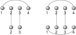
Figure 18. J⁡(1,4,2,3)J(1,4;2,3) has the property that J⁡(1,4,2,3)⊂J⁡(1,4,1,4)J(1,4;2,3)\subset J(1,4;1,4) but J⁡(1,4,2,3)∉TJ​(1,4,1,4)J(1,4;2,3)\not\in T_{J}(1,4;1,4).

4. From the decomposition tree to the partition function

We discussed in the introduction the concept of the loop-based partition function of RNA secondary structures due to McCaskill [20]. We observed there that the key property for its derivation is the unique decomposition into substructures and their recursive analysis. For instance, suppose we are given a tight of type ▽\bigtriangledown from which we remove, by virtue of Cor. 2.2, its outer arc. For this purpose, the context of the latter, i.e. its particular arc-configuration has to be taken into account. However, once the unique decomposition is established, the existence of specific subclasses of joint structures allowing for the dynamic programming of the partition function follows. We remark that the particular choice of the latter may not be unique.

The first step is to extend the standard loop-energy model for secondary structures by introducing two new loop-types due to Chitsaz et al. [11]: the kissing loop and the hybrid, see Figure 19.

4.1. Loops

Having discussed the standard loop types of secondary structures in Section 1, we proceed now by introducing the loops that contain exterior arcs.
(4) a hybrid-loop (𝖧𝗒{\sf Hy})is a sequence ((R⁡[i1],S⁡[j1]),…,([R⁡[is],S⁡[js]))CLOSE((R[i_{1}],S[j_{1}]),\dots,([R[i_{s}],S[j_{s}])), where s≥2s\geq 2 and (ir,jr)(i_{r},j_{r}) is nested in (i1,j1)(i_{1},j_{1}) such that R⁡[ih+1,ih+1−1]=∅ih+1ih+1−1R[i_{h}+1,i_{h+1}-1]=\varnothing_{i_{h}+1}^{i_{h+1}-1} and S⁡[jh+1,jh+1−1]=∅jh+1jh+1−1S[j_{h}+1,j_{h+1}-1]=\varnothing_{j_{h}+1}^{j_{h+1}-1}.
(5) a kissing-loop (𝖪{\sf K}) is either a pair, ((R⁡[i],R⁡[j]),R⁡[i+1,j−1])\left((R[i],R[j]),R[i+1,j-1]\right), such that there exists at least one (R⁡[i],R⁡[j])(R[i],R[j])-child, (R⁡[i1],S⁡[j1])(R[i_{1}],S[j_{1}]) where i<i1<ji<i_{1}<j or a pair ((S⁡[i],S⁡[j]),S⁡[i+1,j−1])\left((S[i],S[j]),S[i+1,j-1]\right), with (R⁡[i],R⁡[j])(R[i],R[j])-child (R⁡[i1],S⁡[j1])(R[i_{1}],S[j_{1}]) and i<j1<ji<j_{1}<j.

Refer to caption

Figure 19. The two new loop types: the hybrid (top) and the kissing loop (bottom).

The arguments of Prop. 2.1, Cor. 2.2, Cor. 2.3 and Cor. 2.4 imply that each joint structure can uniquely be decomposed into a sequence of loops–a necessary and sufficient condition for the mfe-folding of joint structures. As we shall see in the next section, the unique decomposition and the particular choice of loops give rise to specific subclasses via which the partition function can be recursively expressed. Furthermore, following [7], we allow for an initiation energy, i.e. each hybrid loop is given an energy penalty of σ0\sigma_{0}. In addition, we allow for a scaling, 0<σ≤10<\sigma\leq 1, of the energy contribution of each hybrid loop. As default we set σ0=0\sigma_{0}=0, σ=1\sigma=1.

4.2. Case studies

Consider a joint structure J⁡(i,j,h,ℓ)∈T⁡(J⁡(1,N,1,M))J(i,j;h,\ell)\in T(J(1,N;1,M)). For the purpose of assigning an energy to a substructure, we have to distinguish substructures by their “outer” loop type, see Case 11 as well as Fig. 2 and Fig 19. To convey the key ideas we shall restrict our analysis to three case studies.

Refer to caption  

Figure 20. Context dependency: the labels “𝖤,𝖬,𝖥,𝖪{\sf E},{\sf M},{\sf F},{\sf K}” are defined in Case 11. We display from left to right J▽𝖤​(i,j,h,ℓ)J^{{\sf E}}_{\bigtriangledown}(i,j;h,\ell), J▽𝖬​(i,j,h,ℓ)J^{\sf{M}}_{\bigtriangledown}(i,j;h,\ell), J▽𝖥​(i,j,h,ℓ)J^{\sf{F}}_{\bigtriangledown}(i,j;h,\ell) and J▽𝖪​(i,j,h,ℓ)J^{\sf{K}}_{\bigtriangledown}(i,j;h,\ell), respectively.

Given a joint structure J⁡(i,j,h,ℓ)∈T⁡(J⁡(1,N,1,M))J(i,j;h,\ell)\in T(J(1,N;1,M)), we set MR​(i,j)={(R⁡[i1],R⁡[j1])∣i1<i≤j<j1}M_{R}(i,j)=\{(R[i_{1}],R[j_{1}])\mid i_{1}<i\leq j<j_{1}\} and MS​(h,ℓ)={(S⁡[i1],S⁡[j1])∣i1<h≤ℓ<j1}M_{S}(h,\ell)=\{(S[i_{1}],S[j_{1}])\mid i_{1}<h\leq\ell<j_{1}\}.

Case 11. Suppose we are given a tight structure J▽​(i,j,h,ℓ)J_{\bigtriangledown}(i,j;h,\ell). In case of MS​(h,ℓ)=∅M_{S}(h,\ell)=\varnothing, we call S⁡[h,ℓ]S[h,\ell] external and use the notation J▽𝖤​(i,j,h,ℓ)J^{{\sf E}}_{\bigtriangledown}(i,j;h,\ell). Otherwise, let (S⁡[i0],S⁡[j0])(S[i_{0}],S[j_{0}]) be the minimal element of MS​(h,ℓ)M_{S}(h,\ell). We denote the type of the loop including (S⁡[i0],S⁡[j0])(S[i_{0}],S[j_{0}]), by ξ\xi. In case of ξ=𝖬\xi={\sf M}, we use the notation J▽𝖬​(i,j,h,ℓ)J^{{\sf M}}_{\bigtriangledown}(i,j;h,\ell). Otherwise, in case of ξ=𝖪\xi={\sf K}, we write J▽𝖪​(i,j,h,ℓ)J^{{\sf K}}_{\bigtriangledown}(i,j;h,\ell) or J▽𝖥​(i,j,h,ℓ)J^{{\sf F}}_{\bigtriangledown}(i,j;h,\ell) depending on whether or not J▽​(i,j,h,ℓ)J_{\bigtriangledown}(i,j;h,\ell) contains the child of (S⁡[i0],S⁡[j0])(S[i_{0}],S[j_{0}]), see Fig. 20.

Refer to caption  

Figure 21. The twelve subclasses of JD​T​(i,j,h,ℓ)J_{DT}(i,j;h,\ell) as discussed in Case 22.

Case 22. Suppose we are given a double-tight structure, JD​T​(i,j,h,ℓ)J_{DT}(i,j;h,\ell). Then we arrive at the twelve subclasses presented in Figure 21. Indeed, according to Cor. 2.2, there does not exist any JD​T𝖤,𝖤​(i,j,h,ℓ)J_{DT}^{{\sf E},{\sf E}}(i,j;h,\ell), i.e. MR​(i,j)∪MS​(h,ℓ)≠∅M_{R}(i,j)\cup M_{S}(h,\ell)\neq\varnothing. Without loss of generality, we may assume that MR​(i,j)≠∅M_{R}(i,j)\neq\varnothing and that (R⁡[i1],R⁡[j1])∈MR​(i,j)(R[i_{1}],R[j_{1}])\in M_{R}(i,j) is minimal. In case of MS​(h,ℓ)=∅M_{S}(h,\ell)=\varnothing, we use the notation JD​TY,𝖤​(i,j,h,ℓ)J_{DT}^{Y,{\sf E}}(i,j;h,\ell), where YY is the loop type formed by (R⁡[i1],R⁡[j1])(R[i_{1}],R[j_{1}]) and R⁡[i1+1,j1−1]R[i_{1}+1,j_{1}-1]. Otherwise, we have MS​(h,ℓ)≠∅M_{S}(h,\ell)\neq\varnothing. Let (S⁡[i2],S⁡[j2])(S[i_{2}],S[j_{2}]) be the minimal element. In this case we use the notation JD​TY1,Y2​(i,j,h,ℓ)J_{DT}^{Y_{1},Y_{2}}(i,j;h,\ell), where Y1Y_{1} and Y2Y_{2} are the loop-types formed by (R⁡[i1],R⁡[j1])(R[i_{1}],R[j_{1}]), R⁡[i1+1,j1−1]R[i_{1}+1,j_{1}-1] and (S⁡[i2],S⁡[j2])(S[i_{2}],S[j_{2}]), S⁡[i2+1,j2−1]S[i_{2}+1,j_{2}-1], respectively, see Fig. 21.

Case 33. In case of a right-tight structure, JR​T𝖪,𝖪​(i,j,h,ℓ)J_{RT}^{{\sf K},\sf{K}}(i,j;h,\ell), we obtain four subclasses. In case of (R⁡[j],S⁡[ℓ])∈JR​T𝖪,𝖪​(i,j,h,ℓ)(R[j],S[\ell])\in J_{RT}^{{\sf K},{\sf K}}(i,j;h,\ell), we say JR​T𝖪,𝖪​(i,j,h,ℓ)J_{RT}^{{\sf K},{\sf K}}(i,j;h,\ell) is (r​B)(rB) and (r​A)(rA), otherwise. Let (R⁡[i1],S⁡[j1])(R[i_{1}],S[j_{1}]) denote the minimal exterior arc in JR​T𝖪,𝖪​(i,j,h,ℓ)J_{RT}^{{\sf K},{\sf K}}(i,j;h,\ell). According to Prop. 2.1, there exists a unique J⁡(i,j,h,ℓ)J(i,j;h,\ell)-tight structure JT​(R⁡[i1],S⁡[j1])J_{T}(R[i_{1}],S[j_{1}]), such that (R⁡[i1],S⁡[j1])∈JT​(R⁡[i1],S⁡[j1])(R[i_{1}],S[j_{1}])\in J_{T}(R[i_{1}],S[j_{1}]). In case of JT​(R⁡[i1],S⁡[j1])J_{T}(R[i_{1}],S[j_{1}]) is of type ∘\circ, i.e. (R⁡[i1],S⁡[j1])(R[i_{1}],S[j_{1}]) itself and R⁡[i,i1]=∅ii1R[i,i_{1}]=\varnothing_{i}^{i_{1}}, S⁡[h,j1]=∅hj1S[h,j_{1}]=\varnothing_{h}^{j_{1}}, we say JR​T𝖪,𝖪​(i,j,h,ℓ)J_{RT}^{{\sf K},{\sf K}}(i,j;h,\ell) is (l​B)(lB) and (l​A)(lA), otherwise. We use the notation JR​T𝖪,𝖪,Y1,Y2​(i,j,h,ℓ)J_{RT}^{{\sf K},{\sf K},Y_{1},Y_{2}}(i,j;h,\ell), if JR​T𝖪,𝖪​(i,j,h,ℓ)J_{RT}^{{\sf K},{\sf K}}(i,j;h,\ell) is (l​Y1)(lY_{1}) and (r​Y2)(rY_{2}), respectively, see Fig. 22.

Refer to caption  

Figure 22. The four subclasses of JR​T𝖪,𝖪​(i,j,h,ℓ)J_{RT}^{{\sf K},{\sf K}}(i,j;h,\ell), see Case 33 for details.

4.3. The partition function

In the previous section we discussed specific subclasses of joint structures. They were designed to facilitate the recursive construction of the partition function. The purpose of this section is to showcase the respective recursions induced by these classes.
Case 11: J▽𝖬​(i,j,r,s)J^{\sf{M}}_{\bigtriangledown}(i,j;r,s). According to Cor. 2.2, we have three cases: J▽​(i,j,r,s)J_{\bigtriangledown}(i,j;r,s) decomposes into either a J⁡(i−1,j+1,r,s)J(i-1,j+1;r,s)-tight structure of type κ\kappa, where κ∈{▽,∘}\kappa\in\{\bigtriangledown,\circ\} or a J⁡(i−1,j+1,r,s)J(i-1,j+1;r,s)-double tight structure and a ms. By definition of J▽𝖬​(i,j,r,s)J^{\sf{M}}_{\bigtriangledown}(i,j;r,s), the case of a J⁡(i−1,j+1,r,s)J(i-1,j+1;r,s)-tight structure of type ∘\circ is impossible. Considering the type of the loop including (R⁡[i],R⁡[j])(R[i],R[j]) and R⁡[i+1,j−1]R[i+1,j-1], we arrive exactly at the four cases, denoted by I1I_{1}, I2I_{2}, I3I_{3} and I4I_{4}, from left to right, displayed in Fig. 23.

Refer to caption  

Figure 23. The four decompositions of J▽𝖬​(i,j,r,s)J^{\sf{M}}_{\bigtriangledown}(i,j;r,s) via Procedure (b), denoted by I1I_{1}, I2I_{2}, I3I_{3} and I4I_{4}, from left to right, respectively.

Let i<h<ℓ<ji<h<\ell<j. According to the recurrences displayed in Fig. 23, the partition function satisfies for J▽𝖬​(i,j,r,s)J^{\sf{M}}_{\bigtriangledown}(i,j;r,s) the following recursion:

(4.1) Q▽𝖬​(i,j,r,s)=∑h,ℓ(Q⁡(I1)+Q⁡(I2)+Q⁡(I3)+Q⁡(I4)),Q^{\sf{M}}_{\bigtriangledown}(i,j;r,s)=\sum_{h,\ell}(Q(I_{1})+Q(I_{2})+Q(I_{3})+Q(I_{4})),

where

Q⁡(I1)\displaystyle Q(I_{1}) =\displaystyle= Q▽𝖬(h,ℓ;r,s)e−𝖨𝗇𝗍(i,j;h,ℓ)/kT,\displaystyle Q_{\bigtriangledown}^{\sf{M}}(h,\ell;r,s)e^{-{\sf Int}(i,j;h,\ell)/kT},
Q⁡(I2)\displaystyle Q(I_{2}) =\displaystyle= QD​T𝖬,𝖬(h,ℓ;r,s)e−(α1+α2)/kT(e−(j−ℓ−1)α3/kT+Q𝗆(i+1,h−1))\displaystyle Q_{DT}^{\sf{M},\sf{M}}(h,\ell;r,s)e^{-(\alpha_{1}+\alpha_{2})/kT}(e^{-(j-\ell-1)\alpha_{3}/kT}+Q^{\sf{m}}(i+1,h-1))
×(e−(h−i−1)α3/kT+Q𝗆(ℓ+1,j−1)),\displaystyle\times(e^{-(h-i-1)\alpha_{3}/kT}+Q^{\sf{m}}(\ell+1,j-1)),
Q⁡(I3)\displaystyle Q(I_{3}) =\displaystyle= QD​T𝖪,𝖬(h,ℓ;r,s)e−(β1+β2)/kT(e−(j−ℓ−1)β3/kT+Q𝗄(i+1,h−1))\displaystyle Q_{DT}^{\sf{K},\sf{M}}(h,\ell;r,s)e^{-(\beta_{1}+\beta_{2})/kT}(e^{-(j-\ell-1)\beta_{3}/kT}+Q^{\sf{k}}(i+1,h-1))
×(e−(h−i−1)β3/kT+Q𝗄(ℓ+1,j−1)),\displaystyle\times(e^{-(h-i-1)\beta_{3}/kT}+Q^{{\sf k}}(\ell+1,j-1)),
Q⁡(I4)\displaystyle Q(I_{4}) =\displaystyle= Q▽𝖬(h,ℓ;r,s)e−(α1+2α2)/kT(Q−(j−ℓ−1)α3/kTQ𝗆(i+1,h−1)\displaystyle Q_{\bigtriangledown}^{\sf{M}}(h,\ell;r,s)e^{-(\alpha_{1}+2\alpha_{2})/kT}(Q^{-(j-\ell-1)\alpha_{3}/kT}Q^{\sf{m}}(i+1,h-1)
+e−(h−i−1)α3/kTQ𝗆(ℓ+1,j−1))+Q𝗆(ℓ+1,j−1)Q𝗆(i+1,h−1)).\displaystyle+e^{-(h-i-1)\alpha_{3}/kT}Q^{\sf{m}}(\ell+1,j-1))+Q^{\sf{m}}(\ell+1,j-1)Q^{\sf{m}}(i+1,h-1)).

Case 2: JD​T𝖪,𝖬​(i,j,h,ℓ)J_{DT}^{{\sf K},{\sf M}}(i,j;h,\ell). According to Procedure (b), a double tight structure decomposes into a J⁡(i,j,h,ℓ)J(i,j;h,\ell)-tight structure, J⁡(i,i1,h,h1)J(i,i_{1};h,h_{1}) and a J⁡(i,j,h,ℓ)J(i,j;h,\ell)-right tight structure, J⁡(i1+1,j,h1+1,ℓ)J(i_{1}+1,j;h_{1}+1,\ell). We observe that the type of the outer loop of S⁡[h,h1]S[h,h_{1}] and S⁡[h1+1,ℓ]S[h_{1}+1,\ell] coincides with that of S⁡[h,ℓ]S[h,\ell], i.e. 𝖬{\sf M}. Analogously, the outer loop of R⁡[i,i1]R[i,i_{1}] and R⁡[i1+1,j]R[i_{1}+1,j], denoted by (R⁡[i0,j0])(R[i_{0},j_{0}]), is of type 𝖪{\sf K}. Furthermore, at least one of the substructures R⁡[i,i1]R[i,i_{1}] and R⁡[i1+1,j]R[i_{1}+1,j] contain the child of (R⁡[i0,j0])(R[i_{0},j_{0}]). Consequently we arrive at the three scenarios labeled by from left to right by J1J_{1}, J2J_{2} and J3J_{3} displayed in Fig. 24.

Refer to caption  

Figure 24. The decomposition of JD​TK,M​(i,j,h,ℓ)J_{DT}^{K,M}(i,j;h,\ell) via Procedure (b). The corresponding three cases are labeled by from left to right by J1J_{1}, J2J_{2} and J3J_{3}, respectively.

Setting

Q△,▽,□𝖪,𝖬​(i,i1,r,j1)=Q△𝖪,𝖬​(i,i1,r,j1)+Q▽𝖪,𝖬​(i,i1,r,j1)+Q□𝖪,𝖬​(i,i1,r,j1),Q_{\bigtriangleup,\bigtriangledown,\square}^{{\sf K},{\sf M}}(i,i_{1};r,j_{1})=Q_{\bigtriangleup}^{{\sf K},{\sf M}}(i,i_{1};r,j_{1})+Q_{\bigtriangledown}^{{\sf K},{\sf M}}(i,i_{1};r,j_{1})+Q_{\square}^{{\sf K},{\sf M}}(i,i_{1};r,j_{1}),

the recursion of the partition function for JD​T𝖪,𝖬​(i,j,h,ℓ)J_{DT}^{{\sf K},{\sf M}}(i,j;h,\ell) is given by:

(4.2) QD​T𝖪,𝖬​(i,j,r,s)=∑i1,j1(Q⁡(J1)+Q⁡(J2)+Q⁡(J3)),Q_{DT}^{{\sf K},{\sf M}}(i,j;r,s)=\sum_{i_{1},j_{1}}(Q(J_{1})+Q(J_{2})+Q(J_{3})),

where

Q⁡(J1)\displaystyle Q(J_{1}) =\displaystyle= Q△,▽,□𝖪,𝖬​(i,i1,r,j1)​QD​T𝖪,𝖬​(i1+1,j1+1,s)\displaystyle Q_{\bigtriangleup,\bigtriangledown,\square}^{{\sf K},{\sf M}}(i,i_{1};r,j_{1})Q_{DT}^{{\sf K},{\sf M}}(i_{1}+1;j_{1}+1,s)
Q⁡(J2)\displaystyle Q(J_{2}) =\displaystyle= OPENQ△,▽,□𝖥,𝖬​(i,i1,r,j1)​QD​T𝖪,𝖬​(i1+1,j1+1,s))\displaystyle Q_{\bigtriangleup,\bigtriangledown,\square}^{{\sf F},{\sf M}}(i,i_{1};r,j_{1})Q_{DT}^{{\sf K},{\sf M}}(i_{1}+1;j_{1}+1,s))
Q⁡(J3)\displaystyle Q(J_{3}) =\displaystyle= Q△,▽,□𝖪,𝖬​(i,i1,r,j1)​QD​T𝖥,𝖬​(i1+1,j1+1,s).\displaystyle Q_{\bigtriangleup,\bigtriangledown,\square}^{{\sf K},{\sf M}}(i,i_{1};r,j_{1})Q_{DT}^{{\sf F},{\sf M}}(i_{1}+1;j_{1}+1,s).

Case 3: JD​T𝖪,𝖪,B,B​(i,j,h,ℓ)J_{DT}^{{\sf{K},\sf{K}},B,B}(i,j;h,\ell). By definition of JD​T𝖪,𝖪,B,B​(i,j,h,ℓ)J_{DT}^{{\sf{K},\sf{K}},B,B}(i,j;h,\ell), we have (R⁡[j],S⁡[ℓ])∈J⁡(i,j,h,ℓ)(R[j],S[\ell])\in J(i,j;h,\ell). We consider the set of exterior arcs in J⁡(i,j−1,r,ℓ−1)J(i,j-1;r,\ell-1), WW. In case of W=∅W=\varnothing, JD​T𝖪,𝖪,B,B​(i,j,h,ℓ)J_{DT}^{{\sf{K},\sf{K}},B,B}(i,j;h,\ell) decomposes into R⁡[i,j−1]R[i,j-1], S⁡[h,ℓ−1]S[h,\ell-1] and (R⁡[j],S⁡[ℓ])(R[j],S[\ell]). This is the leftmost (first) case (L1L_{1}) displayed in Fig. 25. Otherwise, let (R⁡[i1],S⁡[j1])(R[i_{1}],S[j_{1}]) denote the maximal exterior arc in J⁡(i,j−1,r,ℓ−1)J(i,j-1;r,\ell-1). We consider the unique J⁡(i,j,r,ℓ)J(i,j;r,\ell)-tight structure which contains (R⁡[i1],S⁡[j1])(R[i_{1}],S[j_{1}]), denoted by JT​(R⁡[i1],S⁡[j1])J_{T}(R[i_{1}],S[j_{1}]). If JT​(R⁡[i1],S⁡[j1])J_{T}(R[i_{1}],S[j_{1}]) has not type ∘\circ, we have the second case (L2L_{2}) displayed in Fig. 25. Otherwise, depending on whether or not R⁡[j1+1,j−1]=∅j1+1j−1R[j_{1}+1,j-1]=\varnothing_{j_{1}+1}^{j-1} and S⁡[h1+1,ℓ−1]=∅h1+1ℓ−1S[h_{1}+1,\ell-1]=\varnothing_{h_{1}+1}^{\ell-1}, we have the third (L3L_{3}) and fourth case (L4L_{4}), displayed in Fig. 25.

Refer to caption  

Figure 25. The four decomposition scenarios of JD​T𝖪,𝖪,B,B​(i,j,r,s)J^{{\sf{K},\sf{K}},B,B}_{DT}(i,j;r,s) via Procedure (b). We denote the corresponding cases from left to right by L1L_{1}, L2L_{2} L3L_{3} and L4L_{4}, respectively.

Consequently, we arrive at:

(4.3) QD​T𝖪,𝖪,B,B​(i,j,h,ℓ)=∑j1,h1(Q⁡(L1)+Q⁡(L2)+Q⁡(L3)+Q⁡(L4)),Q_{DT}^{{\sf{K},\sf{K}},B,B}(i,j;h,\ell)=\sum_{j_{1},h_{1}}(Q(L_{1})+Q(L_{2})+Q(L_{3})+Q(L_{4})),

where Q⁡(L1)=Qs𝗄​(i,j−1)​Qs𝗄​(h,ℓ−1)Q(L_{1})=Q_{s}^{\sf k}(i,j-1)Q_{s}^{\sf k}(h,\ell-1) and

Q⁡(L2)\displaystyle Q(L_{2}) =\displaystyle= QR​T𝖪,𝖪,B,A​(i,j1,h,h1)​(Q𝗄​(j1+1,j−1)+Q𝗄​(h1+1,ℓ−1)+Q𝗄​(j1+1,j−1)​Q𝗄​(h1+1,ℓ−1))\displaystyle Q_{RT}^{{\sf{K},\sf{K}},B,A}(i,j_{1};h,h_{1})(Q^{\sf{k}}(j_{1}+1,j-1)+Q^{\sf{k}}(h_{1}+1,\ell-1)+Q^{\sf{k}}(j_{1}+1,j-1)Q^{\sf{k}}(h_{1}+1,\ell-1))
Q⁡(L3)\displaystyle Q(L_{3}) =\displaystyle= QR​T𝖪,𝖪,B,B​(i,j1,h,h1)​e−σ0+σ​𝖨𝗇𝗍​(j,ℓ,j1,h1)\displaystyle Q_{RT}^{{\sf{K},\sf{K}},B,B}(i,j_{1};h,h_{1})e^{-\sigma_{0}+\sigma{\sf{Int}}(j,\ell;j_{1},h_{1})}
Q⁡(L4)\displaystyle Q(L_{4}) =\displaystyle= QR​T𝖪,𝖪,B,B​(i,j1,h,h1)​(Q𝗄​(j1+1,j−1)+Q𝗄​(h1+1,ℓ−1)+Q𝗄​(j1+1,j−1)​Q𝗄​(h1+1,ℓ−1))\displaystyle Q_{RT}^{{\sf{K},\sf{K}},B,B}(i,j_{1};h,h_{1})(Q^{\sf{k}}(j_{1}+1,j-1)+Q^{\sf{k}}(h_{1}+1,\ell-1)+Q^{\sf{k}}(j_{1}+1,j-1)Q^{\sf{k}}(h_{1}+1,\ell-1))

5. Base pairing probabilities

We have seen in Section 3 that the probability of a joint structure, J⁡(1,N,1,M)J(1,N;1,M), is given by

(5.1) ℙ(J(1,N;1,M))=1QIe−F(J(1,N;1,M))/kT,\mathbb{P}(J(1,N;1,M))=\frac{1}{Q^{I}}e^{-F(J(1,N;1,M))/kT},

where QI=∑J⁡(1,N,1,M)e−F(J(1,N;1,M))/kTQ^{I}=\sum_{J(1,N;1,M)}e^{-F(J(1,N;1,M))/kT}. In this section, we shall calculate the base pair probabilities (BPP) for interior and exterior arcs. The key idea is here to associate the probability of specific substructures contained in the decomposition tree. In other words, a term QξY1,Y2,Y3,Y4​(i,j,h,ℓ)Q^{Y_{1},Y_{2},Y_{3},Y_{4}}_{\xi}(i,j;h,\ell) in the recursive calculation of the partition function gives rise to the probability ℙξY1,Y2,Y3,Y4​(i,j,h,ℓ)\mathbb{P}^{Y_{1},Y_{2},Y_{3},Y_{4}}_{\xi}(i,j;h,\ell). For instance, ℙR​T𝖬,𝖪,A,B​(i,j,h,ℓ)\mathbb{P}^{{\sf M},{\sf K},A,B}_{RT}(i,j;h,\ell) is, by construction, the sum over all the probabilities of joint structures J⁡(1,N,1,M)J(1,N;1,M) such that J⁡(i,j,h,ℓ)J(i,j;h,\ell) is contained in T⁡(J⁡(1,N,1,M))T(J(1,N;1,M)) and J⁡(i,j,h,ℓ)=JR​T𝖬,𝖪,A,B​(i,j,h,ℓ)J(i,j;h,\ell)={J}^{{\sf M},{\sf K},A,B}_{RT}(i,j;h,\ell). We remark that the above observations reduce the computation of the BPP to a trace-back routine in the decomposition tree, constructed in Section 3.

The basic strategy can be sketched as follows:
(a) derive from the recursion of the partition function the corresponding recursion of the probabilities
(b) partition the substructures according to their respective contribution to the partition function
(c) for each subclass, recursively calculate the probability of substructures via tracing back the decomposition tree.

We recall that Σ0={J⁡(1,N,1,M)∣J⁡(i,j,h,ℓ)∈T⁡(J⁡(1,N,1,M))}\Sigma_{0}=\{J(1,N;1,M)\mid J(i,j;h,\ell)\in T(J(1,N;1,M))\}. The probability ℙ⁡(i,j,h,ℓ)\mathbb{P}(i,j;h,\ell) is given by

(5.2) ℙ⁡(i,j,h,ℓ)=∑J⁡(1,N,1,M)∈Σ0ℙ⁡(J⁡(1,N,1,M)).\mathbb{P}(i,j;h,\ell)=\sum_{J(1,N;1,M)\in\Sigma_{0}}\mathbb{P}(J(1,N;1,M)).

We accordingly set

(5.3) ℙξY1,Y2,Y3,Y4​(i,j,h,ℓ)=∑J⁡(1,N,1,M)∈Λ0ℙ⁡(J⁡(1,N,1,M)),\mathbb{P}^{Y_{1},Y_{2},Y_{3},Y_{4}}_{\xi}(i,j;h,\ell)=\sum_{J(1,N;1,M)\in\Lambda_{0}}\mathbb{P}(J(1,N;1,M)),

where Λ0={J(1,N;1,M)∣J(i,j;h,ℓ)∈T(J(1,N;1,M)),J(i,j;h,ℓ)∈JξY1,Y2,Y3,Y4(i,j;h,ℓ)}\Lambda_{0}=\{J(1,N;1,M)\mid J(i,j;h,\ell)\in T(J(1,N;1,M)),J(i,j;h,\ell)\in J^{Y_{1},Y_{2},Y_{3},Y_{4}}_{\xi}(i,j;h,\ell)\}.

5.1. Base pairing probabilities for RNA secondary structures

In order to illustrate the concept, let us put the calculation of the BPP for secondary structures into the context of our backtracking routine. Given a secondary structure RR of length NN, the probability of RR is given by ℙ(R)=1Qe−F(R)/kT\mathbb{P}(R)=\frac{1}{Q}e^{-F(R)/kT}. In order to calculate the probability of R⁡[i]R[i] being connected to R⁡[j]R[j] in the equilibrium ensemble of structures, ℙ⁡(iR,jR)\mathbb{P}(i_{R},j_{R}), the first objective is to express the probability of this base pair into a sum of probabilities of substructures. Let T⁡(R⁡[1,N])T(R[1,N]) be the decomposition tree of a particular secondary structure R⁡[1,N]R[1,N] via Procedure (c) and Ω⁡(iR,jR)={S∣(R⁡[i],R⁡[j])∈T⁡(S)}\Omega(i_{R},j_{R})=\{S\mid(R[i],R[j])\in T(S)\}. We remark that Ω⁡(iR,jR)\Omega(i_{R},j_{R}) coincides set of secondary structure such that R⁡[i]R[i] is bound with R⁡[j]R[j], see Section 3, Observation 2. Then we have

(5.4) ℙ⁡(iR,jR)=∑S∈Ω⁡(iR,jR)Q⁡(S)Q.\mathbb{P}(i_{R},j_{R})=\frac{\sum_{S\in\Omega(i_{R},j_{R})}Q(S)}{Q}.

Let Rb​(i,j)R^{b}(i,j) denote the set of segments R⁡[i,j]R[i,j] in which R⁡[i]R[i] is connected with R⁡[j]R[j] and R⁡[i,j]∈T⁡(R⁡[1,N])R[i,j]\in T(R[1,N]). By construction, ℙb​(iR,jR)\mathbb{P}^{b}(i_{R},j_{R}) is the probability of Rb​(i,j)R^{b}(i,j). According to Procedure (c), we have ℙ⁡(iR,jR)=ℙb​(iR,jR)\mathbb{P}(i_{R},j_{R})=\mathbb{P}^{b}(i_{R},j_{R}) since (R⁡[i],R⁡[j])∈T⁡(J⁡(1,N,1,M))(R[i],R[j])\in T(J(1,N;1,M)) if and only if the parent of (R⁡[i],R⁡[j])(R[i],R[j]) in the decomposition tree belongs to Rb​(i,j)R^{b}(i,j). Therefore the problem is reduced to the calculation of ℙb​(iR,jR)\mathbb{P}^{b}(i_{R},j_{R}). Inspection of Procedure (c) shows, that for the parent of an element of Rb​(i,j)R^{b}(i,j) we have to distinguish the five cases displayed in Fig. 26.

Refer to caption

Figure 26. Tracing back: for a parent of Rb​(i,j)R^{b}(i,j) we have according to Procedure (c), five cases, labeled from top to bottom by L1L_{1}, L2L_{2}, L3L_{3}, L4L_{4} and L5L_{5}. For a parent of Rm​(i,j)R^{m}(i,j) there are two cases, denoted by M1M_{1} and M2M_{2}.

Let Rm​(i,j)R^{m}(i,j) denote the set of segments R⁡[i,j]∈T⁡(R⁡[1,N])R[i,j]\in T(R[1,N]) such that R⁡[i,j]≠∅ijR[i,j]\neq\varnothing_{i}^{j}, where the outer loop has type 𝖬{\sf M}. Let Rs​(i,j)R^{s}(i,j) denote the set of segments R⁡[i,j]∈T⁡(R⁡[1,N])R[i,j]\in T(R[1,N]). In particular, Rs​(1,N)=R⁡[1,N]R^{s}(1,N)=R[1,N]. Set ℙm​(iR,jR)\mathbb{P}^{m}(i_{R},j_{R}) and ℙs​(iR,jR)\mathbb{P}^{s}(i_{R},j_{R}) be the probability of Rm​(i,j)R^{m}(i,j) and Rs​(i,j)R^{s}(i,j), respectively. Then we have ℙb​(i,j)=ℙ⁡(L1)+ℙ⁡(L2)+ℙ⁡(L3)+ℙ⁡(L4)+ℙ⁡(L5)\mathbb{P}^{b}(i,j)=\mathbb{P}(L_{1})+\mathbb{P}(L_{2})+\mathbb{P}(L_{3})+\mathbb{P}(L_{4})+\mathbb{P}(L_{5}), where

ℙ⁡(L1)\displaystyle\mathbb{P}(L_{1}) =\displaystyle= ∑h,ℓℙs​(h,ℓ)​Qs​(h,i−1)​Qb​(i,j)Qs​(h,ℓ)\displaystyle\sum_{h,\ell}\mathbb{P}^{s}(h,\ell)\frac{Q^{s}(h,i-1)Q^{b}(i,j)}{Q^{s}(h,\ell)}
ℙ⁡(L2)\displaystyle\mathbb{P}(L_{2}) =\displaystyle= ∑h,ℓℙb​(h,ℓ)​Qb(i,j)e−𝖨𝗇𝗍(i,j;h,ℓ)/kTQb​(h,ℓ)\displaystyle\sum_{h,\ell}\mathbb{P}^{b}(h,\ell)\frac{Q^{b}(i,j)e^{-{\sf Int}(i,j;h,\ell)/kT}}{Q^{b}(h,\ell)}
ℙ⁡(L3)\displaystyle\mathbb{P}(L_{3}) =\displaystyle= ∑h,ℓℙb​(h,ℓ)​Qb(i,j)e−(α1+2α2+(ℓ−j−1)α3)/kTQm(h+1,i−1)Qb​(h,ℓ)\displaystyle\sum_{h,\ell}\mathbb{P}^{b}(h,\ell)\frac{Q^{b}(i,j)e^{-(\alpha_{1}+2\alpha_{2}+(\ell-j-1)\alpha_{3})/kT}Q^{m}(h+1,i-1)}{Q^{b}(h,\ell)}
ℙ⁡(L4)\displaystyle\mathbb{P}(L_{4}) =\displaystyle= ∑h,ℓℙm​(h,ℓ)​Qb(i,j)e−((i−h+ℓ−j)α3+α2)/kTQm​(h,ℓ)\displaystyle\sum_{h,\ell}\mathbb{P}^{m}(h,\ell)\frac{Q^{b}(i,j)e^{-((i-h+\ell-j)\alpha_{3}+\alpha_{2})/kT}}{Q^{m}(h,\ell)}
ℙ⁡(L5)\displaystyle\mathbb{P}(L_{5}) =\displaystyle= ∑h,ℓℙm​(h,ℓ)​Qb(i,j)e−((ℓ−j)α3+α2)/kTQm(h,i−1)Qm​(h,ℓ).\displaystyle\sum_{h,\ell}\mathbb{P}^{m}(h,\ell)\frac{Q^{b}(i,j)e^{-((\ell-j)\alpha_{3}+\alpha_{2})/kT}Q^{m}(h,i-1)}{Q^{m}(h,\ell)}.

Accordingly, the recurrence formulae for ℙm​(i,j)\mathbb{P}^{m}(i,j) and ℙs​(i,j)\mathbb{P}^{s}(i,j) are given as follows:

ℙm​(i,j)\displaystyle\mathbb{P}^{m}(i,j) =\displaystyle= ℙ⁡(M1)+ℙ⁡(M2)\displaystyle\mathbb{P}(M_{1})+\mathbb{P}(M_{2})
ℙ⁡(M1)\displaystyle\mathbb{P}(M_{1}) =\displaystyle= ∑h,ℓℙb​(i−1,ℓ)​e−(α1+2α2+(ℓ−1−h)α3)/kTQb(j+1,h)Qm(i,j)Qb​(i−1,ℓ)\displaystyle\sum_{h,\ell}\mathbb{P}^{b}(i-1,\ell)\frac{e^{-(\alpha_{1}+2\alpha_{2}+(\ell-1-h)\alpha_{3})/kT}Q^{b}(j+1,h)Q^{m}(i,j)}{Q^{b}(i-1,\ell)}
ℙ⁡(M2)\displaystyle\mathbb{P}(M_{2}) =\displaystyle= ∑h,ℓℙm​(i,ℓ)​Qm​(i,j)​Qb​(j+1,h)Qm​(i,ℓ)\displaystyle\sum_{h,\ell}\mathbb{P}^{m}(i,\ell)\frac{Q^{m}(i,j)Q^{b}(j+1,h)}{Q^{m}(i,\ell)}
ℙs​(i,j)\displaystyle\mathbb{P}^{s}(i,j) =\displaystyle= ∑h,ℓℙs​(i,ℓ)​Qs​(i,j)​Qb​(j+1,h)Qs​(i,ℓ).\displaystyle\sum_{h,\ell}\mathbb{P}^{s}(i,\ell)\frac{Q^{s}(i,j)Q^{b}(j+1,h)}{Q^{s}(i,\ell)}.

5.2. Base pairing probabilities for joint structures

Following the basic strategy, we first express the BPP via the probabilities of particular substructures. In the following, we abbreviate J⁡(1,N,1,M)J(1,N;1,M) by JJ. In order to calculate ℙ⁡(iR,jR)\mathbb{P}(i_{R},j_{R}), let Σ1={J∣(R⁡[i],R⁡[j])∈J}\Sigma_{1}=\{J\mid(R[i],R[j])\in J\}, we consider the parent of (R⁡[i],R⁡[j])(R[i],R[j]) in the T⁡(J)T(J) and accordingly obtain

(5.5) Σ1={J∣Rb​[i,j]∈T⁡(J)}∪⋃h,ℓ{J∣J▽​(i,j,h,ℓ)∈T⁡(J)}∪⋃h,ℓ{J∣J□​(i,j,h,ℓ)∈T⁡(J)},\Sigma_{1}=\{J\mid R^{b}[i,j]\in T(J)\}\cup\bigcup_{h,\ell}\{J\mid J_{\bigtriangledown}(i,j;h,\ell)\in T(J)\}\cup\bigcup_{h,\ell}\{J\mid J_{\square}(i,j;h,\ell)\in T(J)\},

which immediately leads to

(5.6) ℙ⁡(iR,jR)=ℙb​(iR,jR)+∑h,ℓℙ▽​(i,j,h,ℓ)+∑h,ℓℙ□​(i,j,h,ℓ),\mathbb{P}(i_{R},j_{R})=\mathbb{P}^{b}(i_{R},j_{R})+\sum_{h,\ell}\mathbb{P}_{\bigtriangledown}(i,j;h,\ell)+\sum_{h,\ell}\mathbb{P}_{\square}(i,j;h,\ell),

where

(5.7) ℙ▽​(i,j,h,ℓ)\displaystyle\mathbb{P}_{\bigtriangledown}(i,j;h,\ell) =\displaystyle= ℙ▽E​(i,j,h,ℓ)+ℙ▽M​(i,j,h,ℓ)+ℙ▽K​(i,j,h,ℓ)+ℙ▽F​(i,j,h,ℓ),\displaystyle\mathbb{P}^{E}_{\bigtriangledown}(i,j;h,\ell)+\mathbb{P}^{M}_{\bigtriangledown}(i,j;h,\ell)+\mathbb{P}^{K}_{\bigtriangledown}(i,j;h,\ell)+\mathbb{P}^{F}_{\bigtriangledown}(i,j;h,\ell),
(5.8) ℙ□​(i,j,h,ℓ)\displaystyle\mathbb{P}_{\square}(i,j;h,\ell) =\displaystyle= ℙ□E​(i,j,h,ℓ)+ℙ□M​(i,j,h,ℓ)+ℙ□K​(i,j,h,ℓ)+ℙ□F​(i,j,h,ℓ).\displaystyle\mathbb{P}^{E}_{\square}(i,j;h,\ell)+\mathbb{P}^{M}_{\square}(i,j;h,\ell)+\mathbb{P}^{K}_{\square}(i,j;h,\ell)+\mathbb{P}^{F}_{\square}(i,j;h,\ell).

Analogously, for ℙ⁡(iS,jS)\mathbb{P}(i_{S},j_{S}) we set

(5.9) Σ2={J∣Sb​[h,ℓ]∈T⁡(J)}∪⋃i,j{J∣J△​(i,j,h,ℓ)∈T⁡(J)},\Sigma_{2}=\{J\mid S^{b}[h,\ell]\in T(J)\}\cup\bigcup_{i,j}\{J\mid J_{\bigtriangleup}(i,j;h,\ell)\in T(J)\},

and obtain

(5.10) ℙ⁡(iS,jS)=ℙb​(hS,ℓS)+∑h,ℓℙ△​(h,ℓ,i,j),\mathbb{P}(i_{S},j_{S})=\mathbb{P}^{b}(h_{S},\ell_{S})+\sum_{h,\ell}\mathbb{P}_{\bigtriangleup}(h,\ell;i,j),

where

(5.11) ℙ△​(h,ℓ,i,j)=ℙ△E​(h,ℓ,i,j)+ℙ△M​(h,ℓ,i,j)+ℙ△K​(h,ℓ,i,j)+ℙ△F​(h,ℓ,i,j).\mathbb{P}_{\bigtriangleup}(h,\ell;i,j)=\mathbb{P}^{E}_{\bigtriangleup}(h,\ell;i,j)+\mathbb{P}^{M}_{\bigtriangleup}(h,\ell;i,j)+\mathbb{P}^{K}_{\bigtriangleup}(h,\ell;i,j)+\mathbb{P}^{F}_{\bigtriangleup}(h,\ell;i,j).

We remark that the expressions for the BPP ℙ⁡(iR,jR)\mathbb{P}(i_{R},j_{R}) and ℙ⁡(iS,jS)\mathbb{P}(i_{S},j_{S}) are not symmetric. This is due to the fact that in our decomposition routines always the outer arcs contained in RR are given preference. In other words, the asymmetry is a result of our particular construction. Finally, we calculate the binding probability of an exterior arc (R⁡[i],S⁡[j])(R[i],S[j]). Since (R⁡[i],S⁡[j])(R[i],S[j]), being a tight structure of type ∘\circ, is already substructure, we can skip the first two steps of the basic strategy. In order to compute the binding probabilities of both: interior and exterior arcs, the key is to employ an “inverse” grammar induced by tracing back in the decomposition tree as displayed in Fig. 27. By virtue of this backtracking, we obtain the recurrence formulae in analogy to the case of secondary structures, discussed above.

Refer to caption

Figure 27. Illustration of the “inverse” grammar, obtained by back-tracing in the decomposition tree.

6. Synopsis

In this paper we derive the partition function and the base pairing probabilities of RNA interaction structures. Furthermore we present the algorithm rip that computes the partition function and the base pairing probabilities in O⁡(N4​M2)+O⁡(N2​M4)O(N^{4}M^{2})+O(N^{2}M^{4}) time and O⁡(N2​M2)O(N^{2}M^{2}) space.

While the partition function is due to [11] our construction is independently derived and based on two ideas: the concept of tight structure in Section 1 and the decomposition tree, presented in Section 3. We did however, adopt the notions of kissing and hybrid loops from [11]. The derivation of the base pairing probabilities for joint structures is new. Here the key idea is to express the latter via energy-wise “quantifiable” substructures, that are contained in the decomposition tree. We discussed that in contrast to the computation of the base pairing probabilities of secondary structures, the specific construction of the unique grammar factors in. As a result, being a joint substructure containing a certain base pair, is not the correct criterion any more. Only those substructures that are obtained via tracing back in the decomposition tree contribute to the base pairing probability.

The complete set of partition function recursions and all details on the particular implementation of rip can be found at

𝚑𝚝𝚝𝚙://𝚠𝚠𝚠.𝚌𝚘𝚖𝚋𝚒𝚗𝚊𝚝𝚘𝚛𝚒𝚌𝚜.𝚌𝚗/𝚌𝚋𝚙𝚌/𝚛𝚒𝚙.𝚑𝚝𝚖𝚕{\tt http://www.combinatorics.cn/cbpc/rip.html}

Finally, we also compute the generating function of joint structures. The analysis of this function is beyond the scope of this paper and can be found as supplemental material at the above web-site.

Refer to caption

Figure 28. The decomposition tree T⁡(1,N,1,M)T(1,N;1,M).

References

  • [1] T. Akutsu. Dynamic programming algorithms for RNA secondary structure prediction with pseudoknots. Disc. Appl. Math., 104:45–62, 2000.
  • [2] C. Alkan, E. Karakoc, J.H. Nadeau, S.C. Sahinalp, and K.Z. Zhang. RNA-RNA interaction prediction and antisense RNA target search. J. Comput. Biol., 13:267–282, 2006.
  • [3] M. Andronescu, Z.C. Zhang, and A. Condon. Secondary structure prediction of interacting RNA molecules. J. Mol. Biol., 345:1101–1112, 2005.
  • [4] J.P. Bachellerie, J. Cavaillé, and A. Hüttenhofer. The expanding snoRNA world. Biochimie, 84:775–790, 2002.
  • [5] D. Banerjee and F. Slack. Control of developmental timing by small temporal RNAs: a paradigm for RNA-mediated regulation of gene expression. Bioessays, 24:119–129, 2002.
  • [6] R. Benne. RNA editing in trypanosomes. the use of guide RNAs. Mol. Biol.Rep., 16:217–227, 1992.
  • [7] S. Bernhart, H. Tafer, U. Mückstein, C. Flamm, P.F. Stadler, and I.L. Hofacker. Partition function and base pairing probabilities of RNA heterodimers. Algorithms Mol. Biol., 1:3–3, 2006.
  • [8] A. Busch, A.S. Richter, and R. Backofen. IntaRNA: efficient prediction of bacterial sRNA targets incorporating target site accessibility and seed regions. Bioinformatics, 24:2849–2856, 2008.
  • [9] W.Y.C. Chen, J. Qin, and C.M. Reidys. Crossings and nestings in tangled diagrams. Electron. J. Comb., 15:R86, 2008.
  • [10] W.Y.C. Chen, J. Qin, C.M. Reidys, and D. Zeilberger. Efficient counting and asymptotics of k-noncrossing tangled diagrams. Electron. J. Comb., 16:R37, 2009.
  • [11] H. Chitsaz, R. Salari, S.C. Sahinalp, and R. Backofen. A partition function algorithm for interacting nucleic acid strands. 2009.
  • [12] A. Fire, S. Xu, and Kostas S.A. Montgomery, M.K. Potent and specific genetic interference by double-stranded RNA in Caenorhabditis elegans. Nature, 391:806–811, 1998.
  • [13] S.M. Hammond, E. Bernstein, D. Beach, and G.J. Hannon. An RNA-directed nuclease mediates pose-transcriptional gene sliencing in drosophlia cells. Nature, 404:293–296, 2000.
  • [14] I.L. Hofacker, W. Fontana, P.F. Stadler, L.S. Bonhoeffer, M. Tacker, and P. Schuster. Fast folding and comparison of RNA secondary structures. Monatsh. Chem., 125:167–188, 1994.
  • [15] J A Howell, T F Smith, and M S Waterman. Computation of generating functions for biological molecules. J Appl Math, 39:119–133, 1980.
  • [16] E.Y. Jin, J. Qin, and C.M. Reidys. Combinatorics of RNA structures with pseudoknots. J. Math. Biol., 70:45–67, 2008.
  • [17] E.Y. Jin and C.M. Reidys. Combinatorial design of pseudoknot RNA. Adv. Appl. Math., 42:135–151, 2009.
  • [18] J. Kugel and J. Goodrich. An RNA transcriptional regulator templates its own regulatory RNA. Nat. Struct. Mol. Biol., 3:89–90, 2007.
  • [19] D. Mathews, J. Sabina, M. Zuker, and D.H. Turner. Expanded sequence dependence of thermodynamic parameters improves prediction of RNA secondary structure. J. Mol. Biol., 288:911–940, 1999.
  • [20] J.S. McCaskill. The equilibrium partition function and base pair binding probabilities for RNA secondary structure. Biopolymers, 29:1105–1119, 1990.
  • [21] M.T. McManus and P.A. Sharp. Gene silencing in mammals by small interfering RNAs. Nature Reiviews, 3:737–747, 2002.
  • [22] U. Mückstein, H. Tafer, S.H. Bernhard, M. Hernandez-Rosales, J. Vogel, P.F. Stadler, and I.L. Hofacker. Translational control by RNA-RNA interaction: Improved computation of RNA-RNA binding thermodynamics. In Mourad Elloumi, Josef Küng, Michal Linial, Robert F. Murphy, Kristan Schneider, and Cristian Toma Toma, editors, BioInformatics Research and Development — BIRD 2008, volume 13 of Comm. Comp. Inf. Sci., pages 114–127, Berlin, 2008. Springer.
  • [23] U. Mückstein, H. Tafer, J. Hackermüller, S.H. Bernhard, P.F. Stadler, and I.L. Hofacker. Thermodynamics of RNA-RNA binding. Bioinformatics, 22:1177–1182, 2006. Earlier version in: German Conference on Bioinformatics 2005, Torda, Andrew and Kurtz, Stefan and Rarey, Matthias (eds.), Lecture Notes in Informatics P-71, pp 3-13, Gesellschaft f. Informatik, Bonn 2005.
  • [24] A. Nykanen, B. Haley, and P.D. Zamore. ATP requirements and small interfering RNA structure in the RNA interference. Cell, 107:309–321, 2001.
  • [25] S. Parrish, J. Fleenor, S. Xu, C. Mello, and A. Fire. A functional anatomy of a dsRNA trigger: Differential requirement for the two trigger strands in RNA interference. Mol. Cell., 6:1077–1087, 2000.
  • [26] J. Qin and C.M. Reidys. A framework for RNA tertiary interaction. 2008.
  • [27] B.J. Reinhart, F.J. Slack, M. Basson, A.E. Pasquinelli, J.C. Bettinger, A.E. Rougvie, H.R. Horvitz, and G. Ruvkun. The 21-nucleotide let-7 RNA regulates developmental timing in Caenorhabdites elegans. Nature, 403:901–906, 2000.
  • [28] J. Ren, B. Rastegari, A. Condon, and H.H. Hoos. Hotknots: heuristic prediction of microRNA secondary structures including pseudoknots. RNA, 11:1494–1504, 2005.
  • [29] E. Rivas and S.R. Eddy. A dynamic programming algorithms for RNA structure prediction including pseudoknots. J. Mol. Biol., 285:2053–2068, 1999.
  • [30] W.R. Schmitt and M.S. Waterman. Linear trees and RNA secondary structure. Disc. Appl. Math., 51:317–323, 1994.
  • [31] E.G.H. Wagner and K. Flardh. Antisense RNAs everywhere? Thends Genet., 244:48–52, 2002.
  • [32] M.S. Waterman and T.F. Smith. RNA secondary structure: A complete mathematical analysis. Math. Biosci, 42:257–266, 1978.
  • [33] M.S. Waterman and T.F. Smith. Rapid dynamic programming algorithms for RNA secondary structure. Adv. Appl. Math., 7:455–464, 1986.
  • [34] D. Yang, H. Lu, and J.W. Erickson. Evidence that processed small dsRNA may mediate sequence-specific mRNA degradation during RNAi in drosophila embryos. Curr. Biol., 10:1191–1200, 2000.
  • [35] D.A. Zorio, K. Lea, and T. Blumenthal. Cloning of caenorhabditis u2af65: an alternatively spliced RNA containing a novel exon. Mol. Cell. Biol., 17:946–953, 1997.