Incorporating Photometric Redshift Probability Density Information into Real-Space Clustering Measurements
Abstract
The use of photometric redshifts in cosmology is increasing. Often, however these photo-s are treated like spectroscopic observations, in that the peak of the photometric redshift, rather than the full probability density function (PDF), is used. This overlooks useful information inherent in the full PDF. We introduce a new real-space estimator for one of the most used cosmological statistics, the 2-point correlation function, that weights by the PDF of individual photometric objects in a manner that is optimal when Poisson statistics dominate. As our estimator does not bin based on the PDF peak it substantially enhances the clustering signal by usefully incorporating information from all photometric objects that overlap the redshift bin of interest. As a real-world application, we measure QSO clustering in the Sloan Digital Sky Survey (SDSS). We find that our simplest binned estimator improves the clustering signal by a factor equivalent to increasing the survey size by a factor of 2–3. We also introduce a new implementation that fully weights between pairs of objects in constructing the cross-correlation and find that this pair-weighted estimator improves clustering signal in a manner equivalent to increasing the survey size by a factor of 4–5. Our technique uses spectroscopic data to anchor the distance scale and it will be particularly useful where spectroscopic data (e.g, from BOSS) overlaps deeper photometry (e.g., from Pan-STARRS, DES or the LSST). We additionally provide simple, informative expressions to determine when our estimator will be competitive with the autocorrelation of spectroscopic objects. Although we use QSOs as an example population, our estimator can and should be applied to any clustering estimate that uses photometric objects.
Keywords:
methods: analytical – methods: statistical – surveys – quasars: general – galaxies: statistics – large-scale structure of Universe.1 Introduction
With the advent of deep and wide multi-band photometric surveys there has been a resurgence of interest in photometric redshifts as a means of estimating the distance to a range of astrophysical objects. Depending on the objects of interest and the information to hand, the derived photometric redshifts will be of varying precision and accuracy, but all can be described by a probability density function (PDF). As our understanding of photometric redshifts improves our confidence in, and ability to characterise, these PDFs, their use in cosmological statistical analyses is sure to increase.
In the sense that photo-s represent color-redshift relations, the use of an ensemble of PDFs for a set of objects is a decades-old approach (e.g. Koo, 1999, and references therein). An example of this is the selection of cluster galaxies (Gladders & Yee, 2000, e.g., via the Red Sequence;). Cluster galaxy selection techniques have, in fact, recently been updated to incorporate full PDFs (van Breukelen & Clewley, 2009) but approaches that use full PDFs remain rare. Subbarao et al. (1996) introduced a method that used Gaussian PDFs to estimate luminosity functions, a problem that has been studied for more arbitrary PDF shapes by Chen et al. (2003) and Sheth (2007). Full PDFs are particularly underutilised in clustering work, where the use of broad redshift bins is more prevalent. By using broad redshift bins to measure photometric clustering one can ameliorate uncertainties in the photo- “peak”, but typically at the expense of constraining power.
One of the most fundamental statistics of any population of objects, and one which carries much physical information, is the 2-point correlation function (Totsuji & Kihara, 1969, e.g.). Provided the redshift distribution of the objects is well known, the underlying 3D clustering can be robustly inferred from the measured clustering in projection (Limber, 1953), but the number of objects required increases dramatically when the redshift distribution is broad. For this reason, estimates of the 2-point function can in principle gain tremendously from improved utilization of the redshift information associated with photometric objects.
Often photo-s are derived from the information in a subset of the objects for which spectroscopy has been obtained. In addition to calibrating the photo-s, this subset of spectroscopic objects can be used as distance anchors with which to set the real-space transverse scale for distances to the photometric objects. Measuring the cross-clustering of photometric objects around spectroscopic objects has several advantages: the properties of the spectroscopic objects, such as luminosity or spectral type are precisely known; the photometric objects are distributed more uniformly, meaning their background clustering signature (the “mask”) is simple to obtain and issues like fiber collisions and more complex hidden selection dependencies that might be introduced by the spectrographic setup are completely absent; the cross-correlation probes the clustering only in a well-defined and localised -range, reducing the sensitivity to photometric outliers while the number of pairs is dramatically increased by using the higher number density of the photometric sample to improve statistics. The use of spectroscopic-photometric cross-correlations to estimate clustering is not new (Longair & Seldner, 1979; Yee & Green, 1984; Yee & Green, 1987; Wold et al., 2000; Hill & Lilly, 1991, e.g.) however, using the information inherent in full PDFs to improve the clustering signal in cross-correlation methods is in its infancy.
In this paper we develop a clustering measure which uses the full photometric redshift PDF and which optimally weights photometric-spectroscopic pairs in the limit that the error is Poisson. Our method circumvents the need to use the peak of the photometric redshift PDF to select which objects lie in a redshift bin of interest, or indeed to bin objects at all. It allows every object that can be assigned a photometric redshift to be usefully cross-correlated against every spectrosopic object in the interval of interest. We also provide simple, informative equations that indicate when photometric redshifts are precise enough, for a given sample size, to provide improved constraints over the spectroscopic auto-correlation. We find that this condition is very hard to satisfy, which explains why even relatively small spectroscopic surveys can produce clustering measurements comparable to much larger photometric samples. We additionally provide a quick method to calculate how much our optimal weighting scheme for spectroscopic-photometric cross-correlations can help satisfy this condition by using full PDF information. The various equations we discuss should be very useful in establishing a survey design to optimise clustering measurements.
To demonstrate our approach with real-world data we apply our new method to measure the clustering of quasars (QSOs). The measurement of QSO clustering sheds light on both QSO demographics and the physics powering these systems. The amplitude of clustering on large scales is related to the masses of the dark matter halos which host the QSOs (their environment), which together with the observed number density allows QSO lifetimes or duty cycles (Cole & Kaiser, 1989; Haiman & Hui, 2001; Martini & Weinberg, 2001) to be constrained. The small-scale clustering of QSOs can shed light on their triggering mechanism, and on the nature of QSO progenitors.
With the advent of large, well-characterised samples, QSOs can now be efficiently photometrically classified (Richards et al., 2004; D’Abrusco et al., 2009; Richards et al., 2009a; Richards et al., 2009b, e.g.) but still have quite imprecise photometric redshifts (Budavári et al., 2001; Richards et al., 2001; Weinstein et al., 2004; Ball et al., 2008, e.g.). This suggests that an estimator that takes full advantage of the information in a photometric redshift might be expected to dramatically improve measurements of the clustering of QSOs. Most previous work on QSO clustering used purely spectroscopic analysis (Porciani, Magliocchetti & Norberg, 2004; Croom et al., 2005; Porciani & Norberg, 2006; Hennawi et al., 2006; Shen et al., 2007; da Angela et al., 2008; Myers et al., 2008), but all such analyses are limited by the extremely low number density of objects with spectra. Higher number densities of objects can be achieved by using photometric QSO selection (Myers et al., 2006; Myers et al., 2007a; Myers et al., 2007b) but systematic errors must be carefully controlled because photometric redshifts for QSOs are still frequently inaccurate. The use of cross-correlations to measure QSO clustering has thus proven quite popular (Croom et al., 2004; Adelberger & Steidel, 2005a; Adelberger & Steidel, 2005b; Serber et al., 2006; Coil et al., 2007; Strand, Brunner & Myers, 2008; Padmanabhan et al., 2009; Mountrichas et al., 2009, e.g.). Our new technique builds on such approaches, particularly that of Padmanabhan et al. (2009), by incorporating new information from photometric PDFs to improve the clustering signal.
We note that, although we choose QSOs as our illustrative data set, our methods and results are significantly more general and our optimal estimator will improve the signal for any real-space clustering measurement that uses photometric redshifts. Although the methods developed in this paper can be easily applied to any spectroscopic-photometric cross-correlation measurement, they will be of particular use in upcoming surveys where sparse spectroscopic data (e.g., from BOSS), is embedded in deeper photometric data, such as from PanSTARRS, DES and the LSST.
The outline of the paper is as follows. §2 introduces our new optimal spectroscopic-photometric cross-clustering estimator. In §3 we introduce the QSO data we use as an example, and in §4 we present the clustering results of this sample and use it to demonstrate the improvement our new technique provides over existing estimators that do not utilise the full PDF. We finish in §5 with some conclusions and lessons learned. We assume a CDM cosmological model with and , consistent with the maximum likelihood estimates from the 5-year WMAP data (Dunkley et al., 2009). All quoted magnitudes are corrected for Galactic extinction using the dust maps of Schlegel, Finkbeiner & Davis (1998).
2 Methodology
2.1 Real Space Clustering Measurements with Photometric Objects
Imagine we have a set of objects for which multi-band photometry has allowed us to estimate photometric redshifts and a second (possibly disjoint) set of objects for which spectroscopic redshifts are available. For the spectroscopic objects we know (up to small uncertainties due to peculiar velocities and uncertainties in the background cosmology) a physical distance to each object, which can be used to anchor the physical scale. Consider the cross-clustering between the set of objects with known spectroscopic redshifts and the set of objects for which only photometric redshifts are known. To begin let us assume that the spectroscopic objects all lie at a single redshift (and hence distance, ) and relax this assumption later. We may estimate11 1 More complex estimators, such as that of Landy & Szalay (1993), could also be used. One would simply substitute each estimator into Eq. (11) or (13) evaluating the terms at different angular positions but at the comoving distance of the spectroscopic data point. We prefer the robustness of Eq. (1) to likely inaccuracies in the spectroscopic “mask” over, e.g., the reduced variance of the Landy & Szalay (1993) estimator. the correlation function using the estimator (Shanks et al., 1983, e.g.)
| (1) |
where we are measuring the cross-clustering of pairs of spectroscopic and photometric objects, “” denotes a data point “” denotes a point drawn from a random catalogue that mimics the data distribution and the subscripts “” and “” denote “photometric” and “spectroscopic”. The factor scales the counts appropriately if the random catalogue has a different size than the photometric catalogue. We denote the random points both to specify that the random distribution mimics the photometric data and to distinguish the term from , the transverse separation. Note that Eq. (1) only requires knowledge of the angular selection function, or “mask”, of the photometric data, not the typically far more complex selection function of the spectroscopic data. We have labeled this estimator because it looks like a normal angular correlation function in the photometric sample, except that angles have been converted to distances using the distance to the spectroscopic partner.
As detailed in Padmanabhan et al. (2009) we infer the projected, real-space, cross-correlation function, , under the assumption that the clustering is constant across the redshift slice and within the Limber (1953) approximation, using the relation
| (2) | |||||
| (3) | |||||
| (4) |
where is the normalised radial distribution function of the photometric objects with and all of the spectroscopic objects lie at . Note that this is a real space measurement and for broad enough we can use the real-space correlation function in the integral, avoiding the need to model redshift-space distortions. Also note that we are making use of the fact that is typically almost constant across the entire line-of-sight range of integration employed in defining . If this is not true then a more sophisticated analysis, which factors in the changing selection function of “random pairs” with distance, is required.
For a distribution of spectroscopic redshifts one replaces in the above with the average, , across the spectroscopic distribution. For a small spectroscopic bin () the redshift distribution will typically be flat. In this case, tells us the fraction of objects in the photometric data set that genuinely have redshifts in the spectroscopic bin of interest () per comoving interval (.
We can use Eq. (4) to answer the question: how large does a photometric sample need to be before a photometric-spectroscopic cross-clustering measurement can compete with a spectroscopic auto-correlation? Clearly, clustering estimates using photometric objects will improve as photometric redshift precision (and accuracy) approaches the level of a spectroscopic redshift (though in this limit our assumption of constant breaks down). In the limit that the objects of interest are rare enough that their clustering is dominated by Poisson shot-noise, then the angular bins in are independent and
| (5) |
where is the number of data pairs in the bin and is for the photometric sample. Note that both and have dimensions of length. Eq. (5) neatly shows the main drawback of spectroscopic-photometric cross-correlation measurements as compared to auto-correlation measurements using only spectroscopic objects. If the photometric redshift solutions are significantly extended along the line-of-sight then is small (perhaps as low as the reciprocal of the depth of the survey). This suppresses the measured clustering, , which for a given sample is proportional to . A very large number of pairs are thus necessary to measure with any precision.
How large is the typical suppression? When measuring the spectroscopic auto-correlation the clustering is integrated along the line-of-sight to eliminate the effects of redshift-space distortions. The limits of integration tend to vary from author to author but typically the line-of-sight interval is . In the language of Eq. (5) such an auto-correlation estimate can approach a limit of . If the photometric sample is extended over, say, Gpc, then , and the number of photometric objects needs to be larger by a factor of in order to measure the clustering as well as if precise redshifts were known. If the extent is Mpc one needs times more objects, and for Mpc one needs times as many. Of course, if obtaining spectroscopy or improved PDFs for the photometric sample is unrealistic then one has no other choice but to use the existing information.
2.2 An Optimal Estimator for Real-Space Clustering using Photometric Redshifts
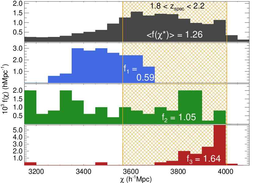
We have noted two major drawbacks to measuring the real-space clustering of photometrically classified objects around spectroscopic objects. First, it is not clear how to establish which photometric objects should be cross-correlated with a given set of spectroscopic objects. The typical approach would be to use objects with a peak photometric redshift solution in the redshift bin of interest. This, however, discards much of the information codified in the photometric redshift PDF and ignores the fact that an object with a peak photometric redshift in the range of interest may actually have less chance of being in that redshift range than an object with a peak photometric redshift beyond that range, particularly as the peak of the PDF may itself be poorly defined. We illustrate this in Figure 1. The second drawback is the possible extension of the ensemble of the photometric redshifts along the line-of-sight, which causes to be small in Eq. (5).

We now introduce a new method designed to circumvent these issues. Consider breaking the photometric sample into very thin slices in photometric redshift, , and labelling the slices from . Each photometric sample, , provides an estimate of via . Writing this estimate as , with an error proportional to in the limit of weak clustering, we can inverse variance weight the different measurements to obtain
| (6) |
where is the number of photometric objects in sample . This circumvents the issue of which photometric objects to cross-correlate against a set of spectroscopic objects in a chosen bin of redshift. Clearly photometric samples which peak at very different redshifts from the spectroscopic sample are significantly down-weighted in the sum. Note that our method also down-weights both objects with unusual colours that might have multi-peaked PDFs and objects with poorly constrained photometry, such as near survey limits, where the PDF might be very broad.
Since the binning is so far arbitrary we can consider the limit where each slice in Eq. (6) represents a single photometric object, i.e. for each . In this case photometric objects that have some overlap with the spectroscopic bin of interest are included in the sum and photometric objects with zero overlap have zero weight. Treating the photometric objects individually, rather than in an ensemble, removes the need for any arbitrary binning and effectively reduces the extension of the ensemble PDF along the line-of-sight and should thus significantly improve the clustering signal-to-noise.
Because the weights in Eq. (6) are a rough determination of how much this new estimator will improve the signal-to-noise of a estimate over existing methods, which only consider objects that have a peak photometric redshift in the bin of interest is
| (7) |
where the subscripts represent our new optimal estimator for a slice containing photometric objects and the represents the number of photometric objects with a PDF peak in the spectroscopic bin of interest. The are the comoving fractional photometric redshift overlaps for objects in slice and is the same for the ensemble of photometric objects with a peak photometric redshift in the spectroscopic bin of interest. This is illustrated in Figure 2, in which the upper panel plots the ensemble of the () PDFs with . This ensemble has an overlap with the true range . The lower panels plot three individual (i.e. ) PDFs and their overlaps with .
2.3 The Optimal Estimator in Practice
In §4, we illustrate the degree to which our optimal estimator can improve clustering estimates for a “typical” analysis, using a sample of spectroscopic and photometric QSOs. QSOs may be particularly well suited to our estimator as they are rare enough that their clustering is dominated by Poisson noise (e.g., see Figure 4) out to reasonably large scales and is quite broad. We note, though, that our optimal estimator should improve the signal-to-noise for any photometric clustering analysis. The exact methodology we use in practice is as follows. Eq (6) can be rewritten as
| (8) |
where
| (9) |
and we have used . Now, consider substituting Eq. (1), the typical estimator for , into Eq. (8)
| (10) |
where the the transverse separation, , is evaluated using the angle between a spectroscopic-photometric pair and the distance to the spectroscopic object. Finally we obtain a simple equation for calculating the real-space clustering of a sample of photometric objects with full PDFs around a sample of spectroscopic objects
| (11) |
The factor reflects the fact that care must be taken to weight the random catalogue correctly, i.e., on a slice-by-slice basis. Note that approximates the reciprocal of from the unweighted estimator. We prefer Eq. (11) to other versions of this expression as it facilitates simple tracking of the data-data counts to construct error estimates from subsampling of the counts.
Finally, we note that one can express the weights in Eq. (9) based on overlaps between each individual spectroscopic and photometric object (i.e. weighting fully by pairs rather than by how much a photometric object overlaps a bin of many spectroscopic objects) without loss of generality. The equations of interest would then reduce to
| (12) |
where is the number of spectroscopic objects in slice . We will choose (as well as ) throughout. Similarly
| (13) |
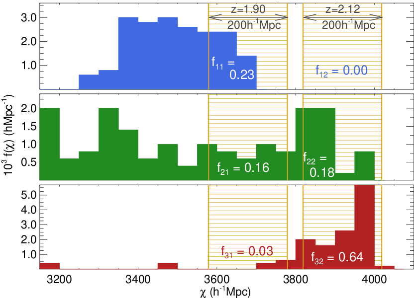
where is the total number of spectroscopic objects analyzed in the spectroscopic bin of interest and is the size of the comoving window integrated over around each spectroscopic object. The additional normalization of arises by analogy with Eq. (11) and the addition of new spectroscopic slices. The extent of the comoving window is entirely flexible, requiring some trial-and-error to determine the optimal choice, although –, as used when integrating out the spectroscopic autocorrelation to eliminate the effects of redshift-space distortions, is an obvious choice. This slightly enhanced approach should provide additional signal-to-noise gains over Eq. (11) provided the photometric PDFs are sufficiently sampled to accurately estimate their overlap with small comoving distance intervals. We illustrate this final, full pair-weighted approach in Figure 3.
3 Data
Although our main result is the new methodology outlined in §2, in §4 we will illustrate our new method with real-world samples to demonstrate the improvements that it can return. We will make use of quasars selected from the SDSS, as described here.
3.1 Photometric Quasars
The photometric quasar sample that we analyze is constructed using the Kernel Density Estimation (KDE) technique of Richards et al. (2004), a technique to classify quasars in photometric surveys which draws on several innovations inherent to the SDSS (e.g., York et al. 2000) – extensive and carefully monitored imaging (e.g., Gunn et al. 1998; Hogg et al. 2001) calibrated to a standard photometric system (e.g., Fukugita et al. 1996; Smith et al. 2002) with a precision of a few-hudredths of a magnitude (Ivezic et al., 2004). These innovations allow quasars to be more easily separated from the stellar locus. We use the DR6 KDE sample, which is detailed in full in Richards et al. (2009a).
The DR6 KDE sample is drawn from a test sample of all point sources in the SDSS DR6 imaging data (Adelman-McCarthy et al., 2008) with , where refers to the asinh magnitude (Lupton, Gunn & Szalay, 1999) in the “uber-calibrated” system of Padmanabhan et al. (2008). The DR6 primary imaging data covers an area of but further cuts (Myers et al., 2006; Richards et al., 2009a) remove approximately or % of the area.
In this paper we concern ourselves only with DR6 KDE objects that have a very high probability of being QSOs. As such, we apply a uvxts=1 cut within the sample. This cut selects QSOs at particularly high efficiency by limiting the DR6 KDE sample to QSOs that would have been selected by traditional UV-excess techniques. As noted in Table 4 of Richards et al. (2009a), and discussed in Myers et al. (2006), only 5% of the uvxts=1 QSOs should, in reality, be stars22 2 Richards et al. (2009a) advocate a good 0 cut to improve efficiency. We ignore this, as for uvxts=1 it only discards a further 2.4% of the data.. The UV-excess nature of the uvxts=1 cut limits the spectroscopic redshift range to .
| 0.8 | 1.0 | 1.2 | 1.4 | 1.6 | 1.8 | 2.0 | 2.2 | |
|---|---|---|---|---|---|---|---|---|
| Imp. | 1.87 | 1.61 | 1.22 | 1.63 | 1.53 | 1.40 | 1.77 | 1.90 |
| (Imp.)2 | 3.50 | 2.60 | 1.48 | 2.65 | 2.35 | 1.96 | 3.15 | 3.63 |
3.1.1 Redshift Distribution of Photometric Quasars
While estimating the redshift of a QSO with a large number of narrow filters can be precise (e.g., Hatziminaoglou et al. 2000; Wolf et al. 2001; Wolf et al. 2003) results using broadband filters are more mixed (e.g., Richards et al. 2001; Budavári et al. 2001). Although photometric redshifts are often expressed as a single value, they are, in reality, probabilistic, with a full probability density function (or PDF) representing the possible redshifts the object of interest could occupy given the filter information. Our main goal in this paper is to incorporate full PDF information into clustering analyses. If we denote by the probability density function for QSO , and assume across all possible redshifts, then the value that will interest us is the fraction of the ensemble PDF that will genuinely lie in any redshift interval
| (14) |
This fraction can be deduced for arbitrary redshift intervals and could correspond to a single photometric QSO () having, say, a 60.3% chance of lying in the redshift range of interest, or equivalently a sample of 100 PDFs in an ensemble from which we might derive that 60.3 of the 100 QSOs in the ensemble can be expected to actually lie in the interval of interest.
We obtain our PDFs using the Nearest Neighbour approach outlined in Ball et al. (2008). We perturb a QSO’s colours relative to a spectroscopic training set drawn from the DR5 QSO sample (Schneider et al., 2007), determine the nearest neighbour over 100 perturbations, and build a function that describes the probability that the photometric quasar matches near spectroscopic neighbours.33 3 Our PDFs for the DR6KDE catalog will be made available at http://lcdm.astro.uiuc.edu/nbckde_dr6_pdfs Examples of these PDFs are shown in Figures 1 and 2.
3.2 Spectroscopic Quasars
We cross correlate the above QSOs with a sample of spectroscopic QSOs drawn from the DR6 QSO sample (Schneider et al. 2009 in prep, see Schneider et al. 2007). Our spectroscopic QSO sample populates the sky in a complex manner but for our method, only the distribution of the photometric sample, which is far simpler, needs to be modeled.
We impose the criterion that our spectroscopic QSOs must also appear in the photometric sample discussed in §3.1. We make no additional cuts on flags or redshift quality, as the vast majority of quasar redshifts are reliable if the object is, indeed, a QSO, and the cuts made by Richards et al. (2009a) help ensure both the quality of the photometry of the QSO, and the likelihood that it is a QSO.
4 Example Implementation of the New Optimal Estimator
In this section, we apply the method developed in §2 to the spectroscopic and photometric QSO samples discussed in §3 to illustrate both our new methodology and its statistical gains over current methods. As our goal is a simple demonstration of our new methodology, we apply no cuts to the samples beyond those discussed in §3. This ensures that any improved signal is due to the method itself, rather than any additional magnitude, colour or redshift cuts that we might impose. As outlined in §3, the only significant cut we employ is the uvxts=1 cut within the photometric sample. This cut, which is purely to ensure that almost all of our photometric objects are genuinely QSOs, limits our spectroscopic redshift range to .
4.1 Expected Improvement in Signal
Eq. (7) allows us to estimate how treating each photometric QSO’s PDF individually (i.e. Eq. 11) will improve the clustering signal over treating the photometric QSOs as an ensemble (as discussed in §2.1). In Figure 2 we demonstrate the calculation of for two different approaches; the ensemble approach of §2.1 and our new bin-weighted approach (Eq. 11), which treats each individually. In Table 1 we show the expected improvement implied by Eq. (7) for a range of spectroscopic redshift bins. This improvement arises from using all of the information inherent in every PDF for every individual photometric object and is about a factor of . Based on Poisson statistics, simply using our new approach should be roughly equivalent to having a – larger survey.
4.2 Actual Improvement in Signal
Poisson errors are typically used to calibrate the noise in a clustering estimator (e.g., Landy & Szalay 1993)
| (15) |
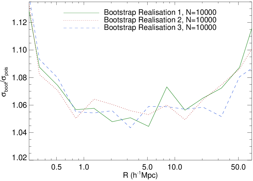
Poisson errors accurately reflect the clustering noise on small scales (where many pairs remain independent) and remain very accurate for the photometric sample being used out to at least (e.g., consider deprojecting Figure 1 of Myers et al. 2006). Poisson errors are more complex to calculate for our new methodology because we incorporate pairs of points with unequal weights, some that may be completely outside the spectroscopic bin of interest, but they can in principle be computed. However we estimate the errors by simply bootstrapping (Efron & Gong, 1983, e.g.,) on the individual spectroscopic QSOs, as was done in Padmanabhan et al. (2009). This approach is additionally useful as it demonstrates how one might estimate errors for our new approach based on other resampling approaches, such as jackknifes or field-to-field variations. Resampling approaches are generally more accurate than Poisson errors on large scales and facilitate the construction of a full covariance matrix. Our preferred expressions for our new estimators (Eq. 11 and 13) make it straightforward to track how each spectroscopic QSO affects the pair counts and quickly construct resampled error estimates.

In Figure 4 we plot the relationship between the Poisson and bootstrap errors derived for the ensemble estimator (i.e., derived using only QSOs with peak PDF solutions in the spectroscopic bin of interest, as discussed in §2.1) using a spectroscopic bin of . Across scales of the bootstrap errors converge to within % for 10,000 bootstraps, and the amplitude of the bootstrap errors closely tracks (within –10%) that of the Poisson errors. This demonstrates that bootstrapping on the spectroscopic QSOs is close to equivalent to using Poisson errors on the scales of interest. On scales , where there are few QSO pairs, more bootstrap samples are likely needed to recreate the precision of the Poisson errors. On scales the Poisson errors likely begin to underestimate the noise as covariance increases.
Having demonstrated the validity of bootstrapping to obtain estimates of the noise we plot the results for the old ensemble approach, our new bin-weighted estimator (Eq. 11) and our full pair-weighted estimator (Eq. 13) in Figure 5. To summarise our results we fit power laws to our data. A power-law 3D correlation function of the form produces a power-law projected correlation function
| (16) |
We fit this form to the measured correlations over the range , using the full bootstrap covariance and holding the index fixed at . In order to improve the numerical stability of this procedure, we scale by , thereby removing the artificially high condition number that arises due to the large dynamic range of . The power-law fit for the old, ensemble, approach gives , our new bin-weighted estimator (Eq. 11) gives () and our full pair-weighted method (Eq. 13) gives (), which agree well with numerous recent estimates of the amplitude of for QSO clustering near (e.g., Porciani, Magliocchetti & Norberg 2004; Croom et al. 2005; Porciani & Norberg 2006; da Angela et al. 2008). We list errors to reflect the fact that our errors are likely underestimated on large scales but the relative improvements for our new estimators are identical whether we quote or errors.
| 0.8 | 1.0 | 1.2 | 1.4 | 1.6 | 1.8 | 2.0 | 2.2 | |
|---|---|---|---|---|---|---|---|---|
| 0.8 | 1.41 | 1.25 | 1.08 | 1.29 | 1.30 | 1.25 | 1.39 | 1.36 |
| 1.3 | 1.43 | 1.28 | 1.11 | 1.34 | 1.27 | 1.21 | 1.35 | 1.44 |
| 2.0 | 1.41 | 1.28 | 1.11 | 1.29 | 1.27 | 1.18 | 1.39 | 1.44 |
| 3.2 | 1.41 | 1.27 | 1.12 | 1.28 | 1.26 | 1.22 | 1.38 | 1.43 |
| 5.1 | 1.42 | 1.29 | 1.13 | 1.30 | 1.26 | 1.21 | 1.36 | 1.43 |
| 8.2 | 1.38 | 1.30 | 1.11 | 1.33 | 1.27 | 1.19 | 1.34 | 1.40 |
| 12.9 | 1.41 | 1.30 | 1.10 | 1.30 | 1.27 | 1.20 | 1.35 | 1.43 |
| 20.5 | 1.38 | 1.28 | 1.11 | 1.28 | 1.26 | 1.20 | 1.33 | 1.36 |
| 10.5 | 1.36 | 1.28 | 1.11 | 1.25 | 1.25 | 1.20 | 1.33 | 1.44 |
It is clear from the fits and errorbars in Figure 5 that our new bin-weighted estimator (Eq. 11), which utilises all of the redshift information in the PDF not just the peak of the PDF, considerably improves the signal-to-noise in estimates of . In Table 2 we list the improvement in signal-to-noise as a function of redshift and scale for our sample. Our new bin-weighted estimator, across scales that are typically used to represent the quasi-linear regime of clustering () improves the signal-to-noise of clustering estimates by 30%. Adopting our most basic approach of incorporating full PDFs into a clustering measurement is thus equivalent to increasing the size of the photometric sample discussed in §3.1 by 60%. Photometric redshift determinations for QSOs in broadband are particularly poor outside of the range . Outside of this range, the improvement yielded by our bin-weighted estimator is slightly larger, equivalent to increasing the survey size by 80%.
We note that our improvements in Table 2 are slightly smaller than the expected improvements listed in Table 1. This could reflect a breakdown in our assumption of Poisson errors or innaccuracy in our PDFs. In fact, one novel approach of our methodology would be to tune the PDFs until the figures in Table 2 peaked, thus constructing PDFs without using any colour information (see also Schneider et al. 2006).
In Table 3 we list the improvement in signal-to-noise as a function of scale using our full pair-weighted estimator (Eq. 13) for a spectroscopic redshift bin of . We adopt a representative range of comoving windows (see the discussion of – near Eq. 13). The improvement in signal-to-noise is about a factor of 2 for scales that are typically used to represent the quasi-linear regime of clustering (). Across some scales the improvement in signal approaches a factor of for a comoving window of . Impressively, this means that our full pair-weighted estimator can potentially improve clustering by a factor equivalent to increasing the size of a survey by a factor of 4–5.
The improvements in Tables 2 and 3 demonstrate that the PDFs we use must carry additional information that can be used to improve clustering signal, which was the main goal of this paper. In future, as our knowledge of PDF construction is refined, the improvements facilitated by our method can only also improve.
| Eq. (11) | Eq. (13); in | |||
|---|---|---|---|---|
| 0.8 | 1.39 | 1.41 | 1.76 | 2.03 |
| 1.3 | 1.35 | 1.39 | 1.80 | 2.10 |
| 2.0 | 1.39 | 1.43 | 1.79 | 2.10 |
| 3.2 | 1.38 | 1.44 | 1.81 | 2.16 |
| 5.1 | 1.36 | 1.42 | 1.76 | 2.05 |
| 8.2 | 1.34 | 1.42 | 1.79 | 2.16 |
| 12.9 | 1.35 | 1.39 | 1.77 | 2.11 |
| 20.5 | 1.33 | 1.34 | 1.70 | 1.99 |
| 10.5 | 1.33 | 1.34 | 1.68 | 2.04 |
5 Conclusions
We have introduced new correlation function estimators to improve measurements of how photometric objects cluster around spectroscopic objects. Spectroscopic-photometric cross-correlations have known benefits, due to the spectroscopic objects having narrowly-defined distance information and the photometric objects having significantly higher number densities. Our approach uses the full photometric probability density information, or PDFs, to optimise such cross-correlation estimates in the Poisson limit. We note that It is possible that a strict Poisson weighting for pairs can be improved upon, particularly on moderate scales.
We have additionally provided simple equations that can be used to calculate when our new estimators will improve on measurements from the spectroscopic autocorrelation. The parameters of interest are the overlap of the photometric data with the spectroscopic bin in comoving space, which depends on the PDF precision, and the relative number of photometric and spectroscopic objects. Because the number of photometric objects scales as the square of the the comoving overlap it can be difficult for spectroscopic-photometric cross-correlations to improve on spectroscopic autocorrelation estimates.
Our improved estimator has several benefits over existing cross-correlation methods. Most obviously, because our estimator does not solely rely on the “peak” of a photometric object’s PDF to determine which photometric objects should be cross-correlated against the spectroscopic objects of interest, the information from more photometric objects is used in clustering estimates. We show that, in the case of photometric QSOs, simply using the bin-weighted form of our estimator (Eq. 11) can thus improve signal-to-noise in the Poisson limit in a manner equivalent to obtaining almost as much survey data. Eq. (7) suggests that the full gains on all scales may be closer to equivalent to obtaining as much survey data. Indeed, our full pair-weighted estimator Eq. (13) demonstrates that gains equivalent to increasing survey size by as much as a factor of 4–5 can be realised. Although we have specifically used the example of QSOs, we stress that our estimator can and should be used to improve the signal for any real-space clustering measurement using photometric redshifts.
The current incarnation of our method has several shortcomings. If the PDFs peak sharply relative to the spectroscopic redshift distribution then cannot be validly extracted, and the full integration across Eq. (2) must be applied. Our assumptions similarly break down if the spectroscopic survey selection function varies rapidly across the redshift bin of interest. In these cases the full 2D correlation function must be integrated in the line-of-sight direction. These inadequacies cannot be countered by narrowing the spectroscopic bin indefinitely, as redshift-space distortions ultimately limit the scale where redshifts map to line-of-sight distances. As such, our assumptions are most robust for the pair-weighted methodology of Eq. (13). In this pair-weighted approach, a strict spectroscopic window of, say, can be enforced, and our assumptions would then be valid until the PDFs are more precise than or the spectroscopic distribution varies rapidly over .
A particular benefit of our estimator is that it can, very simply, incorporate every photometric object into an analysis, negating the need to bin the photometric objects. PDFs of varying precision from a range of photometric data can thus be simply combined in a single measurement, provided the mask of photometric object detections is well-controlled. One could thus envisage taking, say, multi-wavelength photometry from patchy space telescope data or a range of small dedicated surveys (to improve PDFs where possible) embedded in uniform optical photometry such as the SDSS (to establish detections of the photometric objects of interest), and straightforwardly cross-correlating this complex photometric data with a completely different spectroscopic data set. Further, there is no reason to limit the probabilistic information to a photometric redshift. Many techniques, such as star-galaxy separation or the star-QSO separation technique we have used in this paper (Richards et al., 2009a), provide classification probabilities as well as photometric redshifts. Such classification probabilities can naturally be incorporated into our method by, e.g., weighting a PDF heavily to if an object has a high probability of being a star.
Because of the flexibility of our estimator, it should be useful anywhere on the sky where spectroscopic data is embedded in deep, potentially complex and multi-wavelength, photometric data. This should make our estimator particularly useful for regions of the sky where extensive spectroscopy, such as from BOSS, the various 2dF surveys and the SDSS, is embedded in deep, well-calibrated photometry, with measurable PDFs such as from Pan-STARRS, DES and the LSST. Over the next decade, we expect that obvious applications of our estimator will include improved measurements of the clustering of photometric LBGs, LRGs and QSOs around spectroscopic QSOs and measuring the clustering of photometric galaxies and QSOs around absorption features in QSO spectra.
Acknowledgements
ADM was supported in this work by NASA ADP grant NNX08AJ28G and by the University of Illinois. MW is supported by NASA and the DOE. We thank Gordon Richards, Alex Gray, Robert Nichol and Robert Brunner for their substantial and important work in helping produce the KDE photometric QSO catalogue and Nikhil Padmanabhan and Britt Lundgren for helpful conversations.
Funding for the SDSS and SDSS-II has been provided by the Alfred P. Sloan Foundation, the Participating Institutions, the National Science Foundation, the U.S. Department of Energy, the National Aeronautics and Space Administration, the Japanese Monbukagakusho, the Max Planck Society, and the Higher Education Funding Council for England. The SDSS Web Site is http://www.sdss.org.
The SDSS is managed by the Astrophysical Research Consortium for the Participating Institutions. The Participating Institutions are the American Museum of Natural History, Astrophysical Institute Potsdam, University of Basel, University of Cambridge, Case Western Reserve University, University of Chicago, Drexel University, Fermilab, the Institute for Advanced Study, the Japan Participation Group, Johns Hopkins University, the Joint Institute for Nuclear Astrophysics, the Kavli Institute for Particle Astrophysics and Cosmology, the Korean Scientist Group, the Chinese Academy of Sciences (LAMOST), Los Alamos National Laboratory, the Max-Planck-Institute for Astronomy (MPIA), the Max-Planck-Institute for Astrophysics (MPA), New Mexico State University, Ohio State University, University of Pittsburgh, University of Portsmouth, Princeton University, the United States Naval Observatory, and the University of Washington.
References
- Adelberger & Steidel (2005a) Adelberger K.L., Steidel C.C., 2005a, ApJ, 627, L1
- Adelberger & Steidel (2005b) Adelberger K.L., Steidel C.C., 2005b, ApJ, 630, 50
- Adelman-McCarthy et al. (2008) Adelman-McCarthy J.K., et al., 2008, ApJS, 175, 297
- da Angela et al. (2008) da Angela J., et al., 2008, MNRAS, 383, 565
- Ball et al. (2008) Ball N.M., Brunner R.J., Myers A.D., Strand N.E., Alberts S.L.,Tcheng D., 2008, ApJ, 683, 12
- van Breukelen & Clewley (2009) van Breukelen C., Clewley L., 2009, MNRAS, 395, 1845
- Budavári et al. (2001) Budavári, T., et al., 2001, AJ, 122, 1163
- Chen et al. (2003) Chen H.-W., et al., 2003, ApJ, 586, 745
- Coil et al. (2007) Coil A., Hennawi J.F., Newman J.A., Cooper M.C., Davis M., 2007, ApJ, 654, 115
- Cole & Kaiser (1989) Cole S., Kaiser N., 1989, MNRAS, 237, 1127
- Croom et al. (2004) Croom S. M., et al., 2004, in ASP Conf. Ser. 311, AGN Physics with the Sloan Digital Sky Survey, ed. G. T. Richards & P. B. Hall (San Francisco: ASP), 457
- Croom et al. (2005) Croom S.M., et al., 2005, MNRAS, 356, 415
- D’Abrusco et al. (2009) D’Abrusco R., Longo, G., Walton N.A., 2009, MNRAS, 396, 223
- Dunkley et al. (2009) Dunkley J., et al., 2009, ApJS, 180, 306
- Efron & Gong (1983) Efron B., Gong G., 1983, American Statistician, 37, 36
- Fukugita et al. (1996) Fukugita M., Ichikawa T., Gunn J.E., Doi M., Shimasaku K., Schneider, D.P., 1996, AJ, 111, 1748
- Gladders & Yee (2000) Gladders M.D., Yee H.K.C., 2000, AJ, 120, 2148
- Gunn et al. (1998) Gunn J.E., et al., 1998, AJ, 116, 3040
- Haiman & Hui (2001) Haiman Z., Hui L., 2001, ApJ, 547, 27
- Hatziminaoglou et al. (2000) Hatziminaoglou E., Mathez G., Pelló R., 2000, A&A, 359, 9
- Hennawi et al. (2006) Hennawi J.F., et al., 2006, AJ, 131, 1
- Hill & Lilly (1991) Hill G.J., Lilly S.J., 1991, ApJ, 367, 1
- Hogg et al. (2001) Hogg D.W., Finkbeiner D.P., Schlegel D.J., Gunn J.E., 2001, AJ, 122, 2129
- Ivezic et al. (2004) Ivezic Z., et al., 2004, Astron. Nachrichten, 325, 583
- Koo (1999) Koo D.C., 1999, Photometric Redshifts and the Detection of High Redshift Galaxies, 191, 3
- Landy & Szalay (1993) Landy S.D., Szalay A.S., 1993, ApJ, 412, 64
- Limber (1953) Limber D.N., 1953, ApJ, 117, 134
- Longair & Seldner (1979) Longair M.S., Seldner M., 1979, MNRAS, 189, 433
- Lupton, Gunn & Szalay (1999) Lupton R.H., Gunn J.E., Szalay A.S., 1999, AJ, 118, 1406
- Martini & Weinberg (2001) Martini P., Weinberg D.H., 2001, ApJ, 547, 12
- Mountrichas et al. (2009) Mountrichas G., Shanks T., Croom S.M., Sawangwit U., Schneider D.P., Myers A.D., Pimbblet K., 2009, MNRAS, 394, 2050
- Myers et al. (2006) Myers A.D., et al., 2006, ApJ, 638, 622
- Myers et al. (2007a) Myers A.D., Brunner R.J., Nichol R.C., Richards G.T., Schneider D.P., Bahcall N.A., 2007a, ApJ, 658, 85
- Myers et al. (2007b) Myers A.D., Brunner R.J., Richards G.T., Nichol R.C., Schneider D.P., Bahcall N.A., 2007b, ApJ, 658, 99
- Myers et al. (2008) Myers A.D., Richards G.T., Brunner R.J., Schneider D.P., Strand N.E., Hall P.B., Blomquist, J.A., York D.G., 2008, ApJ, 678, 635
- Padmanabhan et al. (2008) Padmanabhan N., et al., 2008, ApJ, 674, 1217
- Padmanabhan et al. (2009) Padmanabhan N., White M., Norberg P., & Porciani C., 2009, MNRAS, 397, 1862
- Porciani, Magliocchetti & Norberg (2004) Porciani C., Magliocchetti M., Norberg P., 2004, MNRAS, 355, 1010
- Porciani & Norberg (2006) Porciani C., Norberg P., 2006, MNRAS, 371, 1824
- Richards et al. (2001) Richards G.T., et al., 2001, AJ, 122, 1151
- Richards et al. (2004) Richards G.T., et al., 2004, ApJS, 155, 257
- Richards et al. (2009a) Richards G.T., Myers A.D., Gray A.G., Riegel R.N., Nichol R.C., Brunner R.J., Szalay A.S., Schneider D.P., Anderson S.F., 2009, ApJS, 180, 67
- Richards et al. (2009b) Richards G.T., et al., 2009, AJ, 137, 3884
- Schlegel, Finkbeiner & Davis (1998) Schlegel D.J., Finkbeiner D.P., Davis M., 1998, ApJ, 500, 525
- Serber et al. (2006) Serber W., Bahcall N., Menard B., Richards G., 2006, ApJ, 643, 68
- Schneider et al. (2006) Schneider M., Knox L., Zhan H., Connolly A., 2006, ApJ, 651, 14
- Schneider et al. (2007) Schneider D.P., et al., 2007, AJ, 134, 102
- Shanks et al. (1983) Shanks T., Bean A.J., Ellis R.S., Fong R., Efstathiou G., Peterson B.A., 1983, ApJ, 274, 529
- Shen et al. (2007) Shen Y., et al., 2007, AJ, 133, 2222
- Sheth (2007) Sheth R.K., 2007, MNRAS, 378, 709
- Smith et al. (2002) Smith J.A., et al., 2002, AJ, 123, 2121
- Strand, Brunner & Myers (2008) Strand N.E., Brunner R.J., Myers A.D., 2008, ApJ, 688, 180
- Subbarao et al. (1996) Subbarao M.U., Connolly A.J., Szalay A.S., Koo, D.C., 1996, AJ, 112, 929
- Totsuji & Kihara (1969) Totsuji H., Kihara, T., 1969, PASJ, 21, 221
- Weinstein et al. (2004) Weinstein M.A., et al., 2004, ApJS, 155, 243
- Wold et al. (2000) Wold M., Lacy M., Lilje P.B., & Serjeant S., 2000, MNRAS, 316, 267
- Wolf et al. (2001) Wolf C., et al., 2001, A&A, 365, 681
- Wolf et al. (2003) Wolf C., Wisotzki L., Borch A., Dye S., Kleinheinrich M., Meisenheimer K., 2003, A&A, 408, 499
- Yee & Green (1984) Yee H.K.C., Green R.F., 1984, ApJ, 280, 79
- Yee & Green (1987) Yee H.K.C., Green, R. F., 1987, ApJ, 319, 28
- York et al. (2000) York D. G., et al., 2000, AJ, 120, 1579