Electronic Transport in Ferromagnetic Conductors with Inhomogeneous Magnetic Order Parameter - Domain-Wall Resistance

We consider a system of effectively non-interacting electrons whose spin degrees of freedom are coupled to the ferromagnetic order parameter in the mean-field approximation via the spatially dependent exchange field. The single particle Hamiltonian has three contributions,

Here, $\mathcal{H}_{0}$ is the usual free quasi-particle energy contribution with the dispersion relation $\epsilon_{{\boldsymbol{k}}}\equiv\frac{\hbar^{2}{\boldsymbol{k}}^{2}}{2M}$ and effective mass $M$ and in spatial representation, ${\boldsymbol{k}}=-i{\boldsymbol{\nabla}}_{{\boldsymbol{r}}}$. $\varphi({\boldsymbol{r}})$ is the external electric potential felt by the quasi-particles of charge $-e$. ${\delta\mu}$ is a shift in the chemical potential due to the magnetization gradient $\partial_{{\boldsymbol{r}}}{\boldsymbol{m}}$ which later turns out to be of order ${\delta\mu}=O(\partial_{{\boldsymbol{r}}}{\boldsymbol{m}})^{2}$. $\mathcal{H}_{\rm S}$ describes the coupling of the electron spin to the exchange field with a constant magnitude $\Delta$ and the local magnetization direction denoted by the unit vector ${\boldsymbol{m}}({\boldsymbol{r}})$. The $2\times 2$ matrix spin structure is denoted by $\hat{\ }$. $\hat{{\boldsymbol{\sigma}}}=(\hat{\sigma}_{1},\hat{\sigma}_{2},\hat{\sigma}_{3})$ is the vector of Pauli matrices, such that the electron spin operator is given by $\hat{{\boldsymbol{S}}}=\frac{\hbar}{2}\hat{{\boldsymbol{\sigma}}}$.

In accordance with the mean-field approach, the length scale of the spatial variations is much slower than the relevant atomic scales. More specifically, this condition reads

The exchange field is created by electrons that align their spin preferably in the same direction due to the (here ferromagnetic) exchange interaction. In conducting ferromagnets, the electrons contributing to the local magnetization can either be localized and, thus, do not participate in transport (d-electron character) or be delocalized and, hence, are subject to electronic transport phenomena (dominant s-electron character). These extreme cases constitute two distinct models with the major difference being the way in which the self-consistency condition for the exchange field is employed. These are known as s-d model and itinerant Stoner model, the latter one describing a system in which transport and magnetism arise in fact both from the same delocalized electrons. However, real physical systems are usually between these two cases. Below, we will restrict ourselves to the s-d model in which the magnetization profile remains static even if the conduction electrons are in a non-equilibrium configuration. Note, that fluctuations of the order parameter are neglected.

We disregard the influence of the effective magnetic exchange field on the electronic orbits, which represents the Lorentz force and leads to the orbital magneto-resistance (OMR). Theoretically, as well as experimentally, the OMR and other extrinsic contributions such as the AMR (anisotropic magneto-resistance), which stems from spin-orbit coupling and leads to a resistance depending on the angle between magnetization and current directions, can be separated from the true DWR and therefore are not included in this article. For Bloch walls and the CPW-geometry (current perpendicular to wall), which we employ in our model later on (see FIG. 1), the AMR plays no role, since the magnetization direction is always perpendicular to the current direction. For other walls like Néel walls, the spin direction within the wall attains a component parallel to the current and the AMR has to be carefully distinguished from the DWR.

The impurity scattering potential can be divided into two contributions,

$\hat{V}_{\rm i}$ describes the scattering from randomly distributed static impurities and for point-like scatterers has the property

equivalent to the treatment of $V_{\rm i}$ as a delta-correlated fluctuating Gaussian field. $\chi^{(i)}$ measures the strength of the impurity scattering potential and $\langle\rangle_{\rm imp}$ denotes the averaging over all impurity configurations.

In a similar way, scattering at impurities that have internal spin-degrees of freedom makes the scattering vertex spin-dependent, such that

Therefore, magnetic impurity scattering in the point-like limit can be treated as delta-correlated fluctuating Gaussian magnetic field which couples to the electron spin by the usual Zeeman term. The size of the fluctuations can be generally spin-anisotropic which manifests itself in the tensor structure of ${\chi^{(m)}_{ij}}$.

The standard way to proceed in non-equilibrium physics is to set up the kinetic equation for the Keldysh Greens function. For the remaining part of this article, we set $\hbar=1$.

The further treatment is done in the Wigner-representation which is obtained from usual spatio-temporal representation via the transformation

The product of operators has to be carried out using the rule

where $\stackrel{{\scriptstyle\leftarrow}}{{\partial}}$ and $\stackrel{{\scriptstyle\rightarrow}}{{\partial}}$ denote derivatives acting only to the left and right, respectively. The transformation (6) introduces center of mass coordinates ${\boldsymbol{r}}$, $t$ and Fourier transformed relative coordinates ${\boldsymbol{k}}$ and $\epsilon$, respectively. Note, that the product $\otimes$ is associative.

The Greens function $\check{G}$ is defined as expectation value of the electron field operators, time-ordered along the Keldysh contour [36]. The ordering along backward and forward time Keldysh contour gives rise to an additional $2\times 2$ matrix structure (denoted by $\check{\ \ }$), which in an appropriate basis takes the convenient form

$\hat{G}^{\rm R}$ and $\hat{G}^{\rm A}$ are the retarded and advanced Greens functions, well known from equilibrium theory and carry information about the spectrum of the system. In particular, one obtains the spectral density simply from

The spectral function generally obeys the normalization condition

The ${\boldsymbol{k}}$-integration of the spectral function yields the density of states, here defined as number of states per unit energy and volume:

The lesser component $\hat{G}^{<}({\boldsymbol{k}},\epsilon,{\boldsymbol{r}},t)$ describes the occupation of states of the many particle system and is given in terms of electron field operators by

where the grandcanonical average is taken and the indices $\alpha,\beta$ are one of ${\uparrow\!,\downarrow}$. In equilibrium, it takes the form

with the Fermi-Dirac distribution function

where $\beta=1/k_{\rm B}T$ denotes the inverse temperature.

From the lesser Greens function $\hat{G}^{<}$ we can easily obtain various physical quantities of interest such as the quasi-particle spin-charge density

and spin-charge current density

where the quasi-particle velocity is ${\boldsymbol{v}}_{k}=\partial_{{\boldsymbol{k}}}\epsilon_{{\boldsymbol{k}}}={\boldsymbol{k}}/m$. The spin-charge density $\hat{N}$ is a $2\times 2$ matrix in spin space and its trace yields the charge-density, $n_{c}=\mathrm{Tr}\hat{N}$ while the spin-density is given by ${\boldsymbol{s}}=-\frac{\hbar}{2e}\mathrm{Tr}(\hat{{\boldsymbol{\sigma}}}\hat{N})$. In a similar manner, we obtain the charge current ${\boldsymbol{j}}_{c}=\mathrm{Tr}\ {\boldsymbol{\hat{J}}}$ and the spin-k current ${\boldsymbol{j}}_{k}=-\frac{\hbar}{2e}\mathrm{Tr}(\hat{\sigma}_{k}{\boldsymbol{\hat{J}}})$.

In order to find $\check{G}$ for a specific physical system, we need an equation of motion, called the Dyson equation, which can be written in the two forms

The self-energy $\hat{\Sigma}$ incorporates scattering by magnetic and non-magnetic impurities. The leading contribution is calculated in the self-consistent Born approximation, which truncates the series of irreducible diagrams due to multiple impurity scattering after the first one:

(18)

In physical terms, this means that all kinds of interference effects like weak localization are dropped from the theory. In this approximation, the self-energy for spin-independent impurity scattering takes the form

Similarly, for magnetic impurity scattering we obtain

The tensorial structure of ${\vbox{\hbox{$\smash{\chi}$}\vskip 1.29167pt\hrule\vskip 0.86108pt\hrule\vskip-2.92773pt}}^{(m)}$ accounts for situations in which scattering is anisotropic in spin space. For example, if an exchange coupling between the internal impurity spin and the ferromagnetic order parameter exists, the spin is preferably aligned along this direction. Consequently, the impurity will scatter the electron with a magnitude depending on its spin. In the case of uniaxial symmetry (the symmetry axis is denoted by ${\boldsymbol{n}}$),

For the above example, the unit vector ${\boldsymbol{n}}$ actually corresponds to the local magnetization direction ${\boldsymbol{m}}$. We assume throughout the rest of this article that scattering is weak such that

where $E_{\rm F}$ is the Fermi energy of the conduction electrons. Put in other words, this means that transport quantities like density of states do vary very slowly on the scale of the relaxation rates given by $\Sigma$. This assumption will allow us later to make use of the quasi-particle approximation.

The first step in solving the Dyson equation (17) is to find a solution for the spectral function. To do so, we write equations for the retarded/advanced components of $\check{G}$,

$\hat{G}^{\rm R/A}$ only differs by the boundary condition which can be simply incorporated by substituting $\epsilon\rightarrow\epsilon\pm i\eta$ in Eqn. (23). Furthermore, since $\Sigma\ll E_{\rm F}$, we will not include impurity self energy corrections to the spectrum, i.e. we neglect the line broadening and assume a delta-peaked spectrum, commonly referred to as the quasi-particle approximation. Also, the external electric field affects the spectrum only in second order of the field.

To proceed, we perform a gradient expansion

and determine $\hat{G}^{\rm R/A}$ iteratively by the order of the gradient. It turns out, that we need only up to order $\partial_{{\boldsymbol{r}}}^{2}$. For example, one finds for the first two terms of the spectral density $\hat{A}=\hat{A}_{0}+\hat{A}_{1}+\dots$.

Here, we defined the projectors in spin-space $\hat{P}_{\uparrow\!,\downarrow}=\frac{1}{2}(\hat{1}\pm{\boldsymbol{m}}\hat{{\boldsymbol{\sigma}}})$ that project on the spin up/down direction and $\epsilon_{{\boldsymbol{k}}}^{\uparrow\!,\downarrow}\equiv\epsilon_{{\boldsymbol{k}}}\mp\frac{\Delta}{2}$ is the dispersion relation for majority and minority spin bands which are exchange split due to the s-d coupling.

The density of states for majority and minority spin bands are

With $\nu_{\uparrow\!,\downarrow}$ without energy argument we denote the density of states at the Fermi-level. The matrix density of states without magnetization gradient present is thus

where we have introduced the polarization of the Fermi surface

and $\nu_{0}=\frac{1}{2}(\nu_{\uparrow}+\nu_{\downarrow})$ denotes the average density of states.

The term ${\delta\mu}$ in Eqs. (23) constitutes an additional chemical potential shift due to the magnetization gradient and is determined by enforcing local charge neutrality. The total quasi-particle density (15) is constant throughout the ferromagnet, i.e. $\mathrm{Tr}{\hat{N}({\boldsymbol{r}})}=-eN_{\rm Ion}$, which leads to

To obtain a kinetic equation for the non-equilibrium distribution function, we subtract the left- and right-conjugated Dyson equations (17),

The equation for the lesser component is

where the (anti-)commutators are defined by $\{\hat{A}\stackrel{{\scriptstyle\otimes}}{{,}}\hat{B}\}=\hat{A}\otimes\hat{B}+\hat{B}\otimes\hat{A}$ and $[\hat{A}\stackrel{{\scriptstyle\otimes}}{{,}}\hat{B}]=\hat{A}\otimes\hat{B}-\hat{B}\otimes\hat{A}$. The imaginary part of the self-energy

describes relaxation due to impurity scattering, while the real part is responsible for changes in the energy dispersion relation. There exists a Kramers-Kronig relation between real and imaginary part,

However, as can be seen from the integral representation in this formula, the real part depends on the complete electronic spectrum of the system, since the scattering rate is directly related to the density of states, $\Gamma(\epsilon)\propto\nu(\epsilon)$. Considering that the dynamics accompanied by a rotation of the magnetization direction, be it in time or space, is affecting only an energy region of the order of $\Delta$, these changes constitute only a tiny fraction of the whole energy range. Thus, corrections due to magnetization dynamics to the real part can be neglected when compared to the whole background contribution, which then is just a constant (however formally diverging due to the assumption of ${\boldsymbol{k}}$-independent impurity scattering) and merely renormalizes the electronic spectrum. In fact, the only reason to include impurity scattering is to add momentum and spin relaxation to the conduction electron system, as contained in the imaginary part of the self-energy, $\hat{\Gamma}$. Therefore, the two commutators involving real parts can be dropped from equation (32).

Generally, we can distinguish the contributions to the kinetic equations emerging from two regions in energy. The electronic states deep inside the Fermi sea are affected by an inhomogeneous exchange splitting $\Delta{\boldsymbol{m}}({\boldsymbol{r}})$. The fraction of the Fermi sea that contributes is given by $\Delta/E_{\rm F}$ and not necessarily small. However, due to the Pauli principle, these states are fully occupied for all reasonable temperatures and the change in the spectrum does not affect the dynamics of the mobile electrons close to the Fermi surface. These are responsible for the dynamics in the quantum kinetic equation, since the electrons in an energy window given by the temperature, voltage or other low-energy scales have the freedom to move. These differences can be used to eliminate the high-energy contribution from our quantum kinetic equation. We perform a series of three steps to obtain an equation describing the low-energy dynamics alone.

First, we eliminate the electric potential by the substitution $\omega=\epsilon+e\varphi$, which transforms the derivatives according to

with the electric field ${\boldsymbol{E}}=-\partial_{{\boldsymbol{r}}}\varphi$.

Secondly, we make the ansatz

The first term drops out from the kinetic equation (32), leaving an equation for $\delta\hat{G}$ alone. $\delta\hat{G}$ has two very practical properties. It is proportional to the electric field, which allows us to drop the term $e\varphi({\boldsymbol{r}})\delta\hat{G}$, since we are interested only in linear response to an external field. The external potential is incorporated via appropriate boundary conditions that are concretized below. Furthermore, $\delta\hat{G}$ is peaked around the Fermi-level, reflecting the fact that non-equilibrium processes take place only in the vicinity of $E_{\rm F}$, provided the temperature is low enough. In fact, we use the zero-temperature approximation $\frac{\partial f_{\rm D}}{\partial\epsilon}=-\delta(\epsilon-E_{\rm F})$ throughout this work.

This brings us directly to the third step which consists of integrating the whole equation over energy after setting $\omega=E_{\rm F}$ in all prefactors to $\delta\hat{G}$ on the right-hand-side of equation (32). The spectral densities in the collision integral become $\hat{A}({\boldsymbol{k}},E_{\rm F},{\boldsymbol{r}})$, which means we neglect the energy-dependence of the scattering rates. This is perfectly compatible with the linear response regime, since a more in-depth investigation shows that corrections due to the energy dependence of $\hat{A}$ are of quadratic order in the electric field.

For the stationary situation ($\partial_{t}=0$), the resulting kinetic equation for

finally reads

The collision integral takes the form

and similar for the magnetic scattering contribution $\hat{\mathcal{I}}_{\rm m}[\hat{g}]$. $\circ$ denotes the Wigner product (7) with derivatives $\partial_{{\boldsymbol{r}}}$ and $\partial_{{\boldsymbol{k}}}$ only, and does not act on ${\boldsymbol{k}}^{\prime}$. Again, we will need to include only terms up to order $\partial_{{\boldsymbol{r}}}^{2}$. Equation (38) along with (39) constitutes a linear integro-differential equation for $\hat{g}$ and serves as the basis for our further analytical treatment.

Provided we have found a solution for $\hat{g}$ with appropriate boundary conditions, we can finally determine the physical observables of interest by simply substituting the ansatz (36) into (15). In this way, we obtain the quasi-particle spin-charge density

with the low-energy spin-charge density excitations $\hat{n}=-e\int\frac{{\rm d}^{3}k}{(2\pi)^{3}}\hat{g}$. We made use of the zero-temperature approximation and smallness of the external potential in the linear regime, viz $f_{\rm D}(\omega-e\varphi)=f_{\rm D}(\omega)+e\varphi\ \delta(\omega-E_{\rm F})$. The (spin-)current is obtained in a similar straightforward manner.

On length scales much larger than the Thomas-Fermi screening length, which is of the order of atomic distances in metallic materials, local charge neutrality is fulfilled. Since the first term on the right-hand side of (40) corresponds to the equilibrium density which exactly neutralizes the material, the trace of the last two terms has to vanish,

Therefore, $\mathrm{Tr}\hat{n}({\boldsymbol{r}})$ is directly related to the local electric potential and thus the local electric field $E({\boldsymbol{r}})=-\partial_{{\boldsymbol{r}}}\varphi({\boldsymbol{r}})$ in the system.

Now we consider a region far from any inhomogenities in the magnetization for which we want to specify an appropriate boundary condition. In the absence of a magnetization gradient and non-equilibrium spin-excitations in the conduction electron system, a less strict equality between the last two terms of (40) holds,

In a simple one-dimensional geometry and at the left and right boundaries $x_{\rm L,R}$, the boundary condition simply becomes

Before continuing to solve the kinetic equation (38) for $\hat{g}$, let us specify a convenient geometry for the contact.

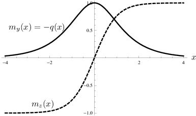
We treat a ferromagnet in a quasi one-dimensional geometry such that there are only gradients of the magnetization in the $x$ direction, while in the $y$- and $z$-directions the system is homogeneous. Furthermore, we assume a coplanar magnetization which allows to parameterize the magnetization direction by a single angle $\theta(x)$, defined by

Current flow perpendicular to the domain wall implies that the direction of ${\boldsymbol{j}}$ is along the $x-$axis, so that the problem becomes effectively one-dimensional. Therefore, in this case, every quantity of interest only depends on $x$, we can set $\partial_{y}=\partial_{z}=0$ and abbreviate $\partial\equiv\partial_{x}$.

The contact of length $L$ contains a domain wall of characteristic width $w$. The left- and rightmost parts have opposite magnetization directions and a so far arbitrary magnetization profile $\theta(x)$ connects the two magnetic domains. The situation is sketched in Fig. 1.

It is then convenient to perform a local SU(2) gauge transformation in order to rotate the coordinate system used to represent the spin-orientation such that its $z$-axis is always aligned to the local magnetization direction ${\boldsymbol{m}}$. The unitary operator ($\hat{\mathcal{U}}^{\dagger}=\hat{\mathcal{U}}^{-1}$)

exactly performs this rotation in spin-space using the previously introduced angle $\theta$, so that $\hat{\mathcal{U}}\ {\boldsymbol{m}}\hat{{\boldsymbol{\sigma}}}\ \hat{\mathcal{U}}^{-1}=\hat{\sigma}_{z}$. As $\theta$ is spatially dependent, the derivatives obtain an additional term after the transformation,

Henceforth, we have to deal with the gradient $q(x)=\partial\theta$ in our equations and which fully parameterizes the domain wall. The gauge transformation (45) rotates the orthonormal basis system $({\boldsymbol{v}}\!\times\!{\boldsymbol{m}},{\boldsymbol{v}},{\boldsymbol{m}})$ such that it becomes the canonical set basis vectors, $({\boldsymbol{e}}_{x},{\boldsymbol{e}}_{y},{\boldsymbol{e}}_{z})$. The unit vector ${\boldsymbol{v}}$ points in the direction of change of the magnetization ${\boldsymbol{m}}$, i.e. $\partial{\boldsymbol{m}}=q{\boldsymbol{v}}$. Note that ${\boldsymbol{v}}$ is perpendicular to ${\boldsymbol{m}}$, since ${\boldsymbol{m}}$ is a unit vector.

An analytical form of the domain wall profile can be derived in the context of minimising the free energy of the ferromagnetic material, commonly a compromise between exchange and anisotropy energy. Typically, one finds

so that

where $w$ constitutes a typical length scale over which the domain wall extends.

In light of the solution procedure that is to come, it is convenient to use a $4$-component vector representation (which is denoted by an arrow to distringuish it from the 3-component real-space vectors set in boldface), in which the spin-charge density excitations and current density take the form, respectively,

Starting from the $2\!\times\!2$-matrix reprentation after the gauge transformation, $\hat{n}=\frac{n_{c}}{2}\hat{1}+n_{x}\hat{\sigma}_{x}+n_{y}\hat{\sigma}_{y}+n_{z}\hat{\sigma}_{z}$, we define the spin-up/down densities $n_{\uparrow\!,\downarrow}=\frac{n_{c}}{2}\pm n_{z}$. Additionally, the transverse spin-degrees of freedom are transformed according to $n_{\pm}=n_{x}\pm in_{y}$, which corresponds to circularly polarized transverse spin excitations. This basis is convenient because it diagonalizes the equations of motion for the transverse dynamics in absence of magnetization gradients, see Eqn. (68) and following.

The full kinetic equation for $\hat{g}$ is still very involved, so we need to perform additional simplifying steps. Therefore, we multiply Eq. (38) with $v_{x}^{n}$ ($n\geq 0$) and afterwards integrate over the whole $k$-space. This involves evaluating terms of the form

and defining moments of the Greens function $\hat{g}$

The first two momenta are $\hat{g}^{(0)}=\hat{n}$ and $\hat{g}^{(1)}=\hat{j}$, obviously. The kinetic equation (38) turns into an infinite hierarchy of equations relating these moments. It is nevertheless possible to find an analytical solution to these equations in form of a systematic series expansion in the function $q(x)$. As we will show below, it is then possible to truncate the hierarchy by setting $\hat{g}^{(5)}=0$ in order to calculate the domain-wall resistance. The first two of these equations are reminiscent of spin-charge continuity and diffusion equations and take the explicit form

where we defined the derivative $\smash{\partial}$   , modified by the SU(2) gauge transformation (see equation (46)),

The right-hand-sides of these equations include important contributions that are due to modification of various transport properties in presence of a magnetization gradient like the change in the density of states which enters the collision integrals. Thus, the right-hand-side vanishes as $q\rightarrow 0$. Their explicit form along with the equations for $\hat{g}^{(2)}$, etc. are rather lengthy and not needed for our following discussion. Further details can be found in the appendix in equations (125)-(133).

The various scattering rates associated with momentum relaxation $\smash{\Pi}$   and spin-flip/-dephasing $\smash{\Gamma}$   are most conveniently expressed, introducing the parameters $\gamma,\kappa$ and $\xi$, in the following way:

Spin precession is incorporated as well and manifests itself as an imaginary part in the entries of the transverse subspace of $\smash{\Gamma}$   and $\smash{\Pi}$   .

In terms of the parameters of our specific model, the various scattering parameters take the form

$\chi$ measures the ratio of momentum relaxation rate to exchange splitting $\Delta$, $\xi$ denotes the transverse spin-dephasing strength and $\gamma$ can be considered as scattering asymmetry parameter while $\kappa$ is the strength of spin-flip scattering.

Of course, the parameter $\gamma$ carries an implicit dependency on the exchange splitting $\Delta$ entering through the polarization parameter

expressed here by the dimensionless exchange splitting ${\tilde{\Delta}}\equiv\frac{\Delta}{2E_{\rm F}}$. Within our specific model of impurity scattering, $\gamma=P(1-\xi\kappa)$ is not independent of the other parameters. It is worth mentioning that this specific form of $\gamma$ has to be employed in order to guarantee for a consistent treatment of the gradient corrections in the collision integral.

Furthermore, the matrix of diffusion constants reads

where we introduced $D_{\perp}=\frac{2E_{\rm F}}{3M}\frac{1}{\gamma_{j}^{\perp}}=\frac{1}{3}v_{\rm F}^{2}\frac{1}{\gamma_{j}^{\perp}}$. Transverse spin excitations are also subject to precession as they diffuse which results in the complex values of the effective transverse diffusion constants.

Finally, let us stress that the reason for the inclusion of the moments up to $\hat{g}^{(4)}$ lies in the fact that in our regime of investigation the precession length $l_{\rm prec}\equiv 2\pi\frac{v_{\rm F}}{\sqrt{3}\Delta}$ is, besides the Fermi-length, the smallest length scale in the system. As can be seen from the equation (III.3), $l_{\rm prec}$ describes the period of oscillation of transverse spin excitations. In the diffusive approximation, as for example used by Bergeret et al [24], the scattering mean free path $l_{\rm s}$ is the smallest length scale in the system (besides the Fermi wave length) and not $l_{\rm prec}$. Hence, it is possible to truncate the hierarchy of equations already by $\hat{g}^{(3)}=0$, which results in only two equations that are just the spin-chage continuity and diffusion equation. The latter is obtained by plugging the equation for $\hat{g}^{(2)}$ into the equation for $\hat{g}^{(1)}$ (see also appendix, for more details).

We eliminate the higher order moments $\hat{g}^{(n\geq 1)}$ by iteratively substituting the equations into each other, carefully keeping terms that contribute up to order $q^{2}$. We find a differential equation for the vector of quasi-particle excitations $\vec{n}$ of the form

where the differential operator ${\vbox{\hbox{$\smash{W}$}\vskip 1.29167pt\hrule\vskip 0.86108pt\hrule\vskip-2.92773pt}}(q)$ vanishes for $q\rightarrow 0$ and contains all possible terms up to order $q^{2}$. In the homogeneous ($q=0$) and collinear case, Eq. (68) corresponds to the transport equation used by Valet and Fert [37]. Let us stress that $\vec{n}$ represents the unscreened spin-charge density excitations, while the true, screened quantity $\vec{n}^{(s)}$ is, according to Eq. (40),

Here, spin-excitations are not screened since our model does not include a spin-dependent interaction.

Generally, ${\vbox{\hbox{$\smash{W}$}\vskip 1.29167pt\hrule\vskip 0.86108pt\hrule\vskip-2.92773pt}}(q)$ contains terms of the form ${\vbox{\hbox{$\smash{Y}$}\vskip 1.29167pt\hrule\vskip 0.86108pt\hrule\vskip-2.92773pt}}_{ijk}\partial^{i}q\partial^{j}q\partial^{k}$, ${\vbox{\hbox{$\smash{Y}$}\vskip 1.29167pt\hrule\vskip 0.86108pt\hrule\vskip-2.92773pt}}_{ij}\partial^{i}q\partial^{j}$ and ${\vbox{\hbox{$\smash{Y}$}\vskip 1.29167pt\hrule\vskip 0.86108pt\hrule\vskip-2.92773pt}}_{i}\partial^{i}$, where the order of $q$ and $\partial$ is crucial, since $\partial$ acts on everything to its right. The constant matrices $\smash{Y}$   that depend on our set of parameters, ${\tilde{\Delta}},\gamma,\xi,\kappa$ can be obtained in a straightforward manner from equations (125)-(129) by collecting all terms associated with the corresponding factor $\partial^{i}q\partial^{j}q\partial^{k}$. Restricted to terms that contribute to DWR, its explicit form (see eqn. (131)) is given in the appendix.

Since we have a perturbative treatment in $q$ in mind, we determine the Greens function of Eq. (68)

Separated into longitudinal (l) and transversal (t) subspace, the Greens function is

Matrices in the $2\!\times\!2$ subspaces are denoted by a single underbar as compared to the double underbar which indicates a $4\!\times\!4$ matrix. The index l and t refers to longitudinal and transverse componenents, respectively, so that for example

The longitudinal component ${\vbox{\hbox{$\smash{G}$}\vskip 0.86108pt\hrule\vskip-1.29167pt}}_{\rm ll}$ consists of two contributions. The first term of ${\vbox{\hbox{$\smash{G}$}\vskip 0.86108pt\hrule\vskip-1.29167pt}}_{\rm ll}$ decribes spatial damping of spin-up/down non-equilibrium excitations which manifests itself in the characteristic exponential decay on the spin-diffusion length,

The second term of ${\vbox{\hbox{$\smash{G}$}\vskip 0.86108pt\hrule\vskip-1.29167pt}}_{\rm ll}$ describes the linear behaviour of the chemical potential in a homogenous system in the absence of a magnetization gradient. The two tensors

obey the useful identities

References

- [1] E. B. Myers, D. C. Ralph, J. A. Katine, R. N. Louie, and R. A. Buhrman, Science 285, 867 (1999).
- [2] S. Urazhdin, N. O. Birge, W. P. Jr Pratt, and J. Bass, Phys. Rev. Lett. 91, 146803 (2003).
- [3] B. Ozyilmaz, A. D. Kent, D. Monsma, J. Z. Sun, M. J. Rooks, and R. H. Koch, Phys. Rev. Lett. 91, 067203 (2003).
- [4] J. Grollier, V. Cros, A. Hamzic, J.M. George, H. Jaffrès, A. Fert, G. Faini, J.B. Youssef, and H. Legall, Appl. Phys. Lett. 78, 3663 (2001).
- [5] J.A. Katine, F. J. Albert, R. A. Buhrman, E. B. Myers, and D.C. Ralph, Phys. Rev. Lett. 84, 4212 (2000).
- [6] G. Tatara, and H. Kohno, Phys. Rev. Lett. 92, 086601 (2004).
- [7] Z. Li, and S. Zhang, Phys. Rev. Lett. 92, 207203 (2004).
- [8] S. Zhang, and Z. Li, Phys. Rev. Lett. 92, 207203 (2004).
- [9] A. Thiaville, Y. Nakatani, J. Miltat, and Y. Suzuki, Europhys. Lett. 69, 990 (2005).
- [10] S.E. Barnes, and S. Maekawa, Phys. Phys. Lett. 95, 107204 (2005).
- [11] S.E. Barnes, J. Ieda, and S. Maekawa, Appl. Phys. Lett. 89, 122507 (2006).
- [12] S. S. P. Parkin, M. Hayashi, and L. Thomas, Science 320, 190 (2008).
- [13] J. C. Slonczewski, J. Magn. Magn. Mater. 159, L1 (1996).
- [14] L. Berger, Phys. Rev. B 54, 9353 (1996).
- [15] M. Tsoi, A. G. M. Jansen, J. Bass, W.-C. Chiang, M. Seck, V. Tsoi, and P. Wyder, Phys. Rev. Lett. 80, 4281 (1998).
- [16] E. B. Myers, D. C. Ralph, J. A. Katine, R. N. Louie, and R. A. Buhrman, Science 285, 867 (1999).
- [17] Y. Tserkovnyak, A. Brataas, G. E. W. Bauer, and B. I. Halperin, Rev. Mod. Phys. 77, 1375 (2005).
- [18] P. Levy and S. Zhang, Phys. Rev. Lett. 79, 5110 (1997).
- [19] G. Tatara and H. Fukuyama, Phys. Rev. Lett. 78, 3773 (1997).
- [20] A. Brataas, G. Tatara, and G. Bauer, Phys. Rev. B 60, 3406 (1999).
- [21] R. P. van Gorkom, A. Brataas, and G. E. W. Bauer, Phys. Rev. Lett. 83, 4401 (1999).
- [22] G. Tatara, Int. J. of Mod. Phys. B 15, 321 (2001).
- [23] V. Dugaev, J. Barnas, A. Lusakowski, and L. Turski, Phys. Rev. B 65, 224419 (2002).
- [24] F. Bergeret, A. Volkov, and K. Efetov, Phys. Rev. B 66, 184403 (2002).
- [25] E. Simanek, Phys. Rev. B 63, 224412 (2001).
- [26] E. Simanek and A. Rebei, Phys. Rev. B 71, 172405 (2005).
- [27] U. Ruediger, J. Yu, S. Zhang, A. Kent, and S. Parkin, Phys. Rev. Lett. 80, 5639 (1998).
- [28] U. Ebels, A. Radulescu, Y. Henry, L. Piraux, and K. Ounadjela, Phys. Rev. Lett. 84, 983 (2000).
- [29] A. Aziz, S. J. Bending, H. G. Roberts, S. Crampin, P. J. Heard, and C. H. Marrows, Phys. Rev. Lett. 97, 206602 (2006).
- [30] C. Hassel, M. Brands, F. Y. Lo, A. D. Wieck, and G. Dumpich, Phys. Rev. Lett. 97, 226805 (2006).
- [31] C. Marrows, Adv. in Phys. 54, 585 (2005).
- [32] A. Kent, J. Yu, U. Rudiger, and S. Parkin, J Phys.-Cond. Mat 13, R461 (2001).
- [33] D. Huertas-Hernando, Yu. V. Nazarov, and W. Belzig, Phys. Rev. Lett. 88, 047003 (2002).
- [34] A. Cottet and W. Belzig, Phys. Rev. B 72, 180503R (2005).
- [35] D. Huertas-Hernando, Yu. V. Nazarov, A. Brataas, and G. E. W. Bauer, Phys. Rev. B 62, 5700 (2000).
- [36] J. Rammer and H. Smith, Rev. Mod. Phys. 58, 323 (1986).
- [37] T. Valet and A. Fert, Phys. Rev. B 48, 7099 (1993).