ANALYTIC ESTIMATION OF THE NON-LINEAR TUNE SHIFT DUE TO THE QUADRUPOLE MAGNET FRINGE FIELD
Abstract
Analytic expressions for the amplitude-dependent tune shift driven by the quadrupole magnet fringe field have been obtained. The magnitude of the effect is compared with other sources of non-linearity such as chromatic sextupoles, octupole errors of the main quadrupole magnetic field and kinematic terms. A numerical example was the calculation on the lattice of the VEPP-4M collider.
1 Introduction
The main sources of non-linear detuning for storage rings and synchrotrons are the low-order multipole components of the magnetic field (sextupole and octupole ones). Many authors investigated the influence of these components on beam dynamics both through numerical simulation and analytically. The expressions estimating the non-linear betatron tune shift for such perturbations are well-known.
There are, however, other sources of the amplitude-tune shift that are able to influence significantly the beam behavior. For instance, the non-linearity of the fringe field was considered in [1] for the low-energy ring (LER) of the PEP-II facility. It was shown that the main contribution (larger than that of the regular chromatic sextupoles) was made by the fringe field of the quadrupole magnets. The kinematic effects and the fringe field of the bending magnets have no significant influence. For the B-factory of KEK [2], it is pointed out that the main limits of the dynamical aperture are determined by the kinematic terms of the interaction point drift space and by the fringe field of the quadrupoles adjacent to the interaction point.
The studies are usually performed by computer simulation when the map over the quadrupole edge is written in terms of the Lee operators [3] or with the help of a second-order matrix formalism [4].
Below is made an attempt to obtain simple analytic expressions for the contribution of the quadrupole magnet fringe field to the non-linear tune shift. The formulae for the kinematic effects and ordinary octupole non-linear detuning are also presented for comparison. The octupole non-linear component is considered here as a small error of an ideal field inside the quadrupole lens. The contribution of perturbations of various kinds is compared on the basis of the VEPP-4M electron-positron storage ring.
2 Hamiltonian
We will consider a quadrupole magnet with an edge field drop (see, for instance, [5]). We will assume that an ideal quadrupole field inside the magnets is disturbed only by an octupole field error. Hence, we will be able to compare its contribution to the nonlinear detuning with that induced by the fringe field effect. The kinematic terms will also be included into the consideration.
The transversal components of the quadrupole magnetic field are expressed as
| (2.1) |
where is the field gradient, is the octupole component and describes the contribution of the fringe field. Since the octupole field and edge field non-linearity are presented by the same power expansion series (but with different signs), the latter is referred to as pseudooctupole non-linearity sometimes.
The Hamiltonian of the transversal motion of an on-energy relativistic electron in a magnetic field (2.1) has the form of [6]:
| (2.2) |
where and . It is considered here that for the horizontally-focusing quadrupole magnet.
The main aim of this work is to investigate the non-linearity of the fringe field. However, for the purpose of comparison and estimation, expressions for the kinematic terms and for the regular octupole component of the magnetic field will be also obtained.
In order to find the amplitude-tune dependence in the first order of approximation, let us write down expressions (2.2) in the ”action-angle” variables [7] with the help of the generating function
| (2.3) |
which assigns the following relations for the old and new variables:
| (2.4) |
where and are the Twiss parameters.
Averaging the new Hamiltonian over all phase variables, , and computing the oscillation tune of the system according to
| (2.5) |
we obtain the following first-order expressions for the amplitude-tune dependence:
| (2.6) |
where the coefficients include the contribution of the kinematic effects, fringe field and regular octupole perturbation: . Coefficients of each type have the following form:
- a)
Kinematic coefficients.
(2.7) where .
- b)
Fringe field coefficients.
(2.8) - c)
Regular octupole component coefficients.
(2.9)
3 Kinematic effects
The main contribution to integral expressions (2.7) is made by the drift space with an extremely small value of the betatron function. The interaction region is best suited to consideration from such point of view (see, for instance, [2]). For a straight section with the length , where behavior of the beta-functions is mirror-symmetric relative to the center, ( is the value at the center of the section), expressions (2.7) take a simple form, convenient for estimation:
| (3.1) |
4 Octupole errors
If the magnet lattice of the accelerator is known and, thus, the behavior of the beta-functions along the beam trajectory is calculated, one can easily compute coefficients (2.9) numerically. However, we obtain the following simple estimation to be able to compare the influence of the octupole error of the central part of a quadrupole lens long with the influence of the fringe fields of this lens.
Let us assume, for the coefficient , that is approximately constant inside the lens () and the octupole component is constant over the length, then
| (4.1) |
The quality of a magnetic field is usually defined as the relative difference between the real and ideal values of the field at the radius (we will regard this radius as the inscribed radius of the aperture of the quadrupole lens). Then, from (2.1) for the field in the median plane () it follows that
| (4.2) |
Substituting (4.2) into (4.1), we obtain the estimation we will need later:
| (4.3) |
5 Fringe fields
The non-linear betatron tune shift caused by the fringe fields of lenses is the principal subject of this work. In order to simplify expression (2.8), we need to introduce a model describing the behavior of the fringe field of the quadrupole lens.
We have considered the following variants of model distribution of the quadrupole lens fringe field: the one based on M.Bassettis’s formulae [8, 9], the model of ”four lines” by G.Lee-Whiting [10] and the description of the magnetic field drop with two matched parabolas [11]. The first two models describe rather precisely the fringe field and its derivatives with respect to the longitudinal coordinate.
For instance, for the ”four-line” model, the distribution of the gradient and its first two derivatives (required for computation of (2.8)) at the edge of the lens has the following form:
| (5.1) | |||||
where is the inscribed radius of the aperture of the lens and is the gradient on the lens axis in the central section. The approximation of the fringe field with the help of (5.1) is shown in Fig.5.1, 5.2. Unfortunately, it is rather complicated to use (5.1) since the field distribution is assumed infinite on each side of the axis (the edge corresponds to ). So, a correct integration of (2.8) with due regard to the real behavior of the betatron function becomes difficult.
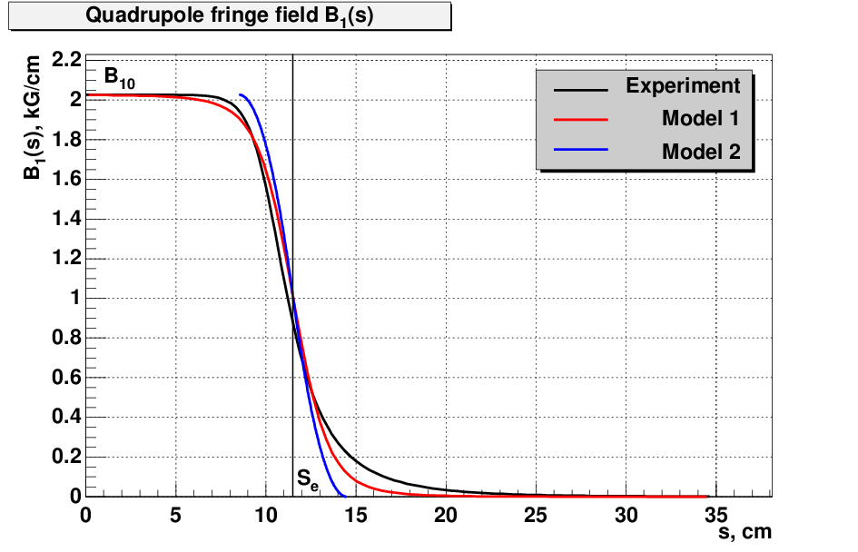
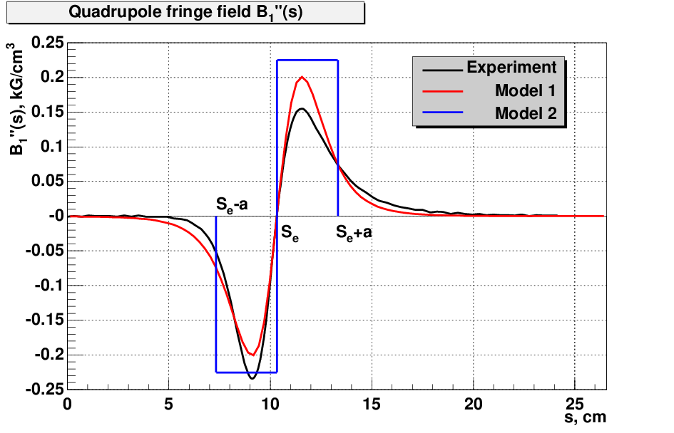
At the same time, a simple model of two matched parabolas [1]
| (5.2) |
yields a rather good approximation of the resulting expressions without cumbersome evaluation of numeric coefficients for the model (5.1). The difference between the value of coefficients for models (5.1) and (5.2) will be shown below.
Fig.5.1, 5.2 present the measured gradient drop of the quadrupole lens [12] and the model expression according to (5.1) and (5.2). The main notations used below are also given. The inscribed radius of the aperture of the lens cm; the maximal gradient at the center of the lens T/m. It is worth noting that because of the quadrupole symmetry the end-pole chamfer, usually used for adjustment of the efficient length of the lens, has practically no influence on the fringe field pseudooctupole component defined by
The fringe effects are concentrated in the vicinity of the longitudinal edge of the lens with a typical region length close to the lens inscribed radius: . We assume that the betatron functions vary a little over this length, so they can be presented in the first-order expansion. For instance, for the horizontal beta-function:
| (5.3) |
where and are the magnitudes of the beta-function and its derivative at the edge and for the first and second edges.
Let us substitute (5.3) and corresponding derivatives of the fringe field (5.2) into (2.8) and perform the integration. Then we can obtain the following expressions describing the contribution of the fringe field of the quadrupole lens to the non-linear shift of the betatron tune:
| (5.4) |
where is the focusing coefficient of the lens at the center. It is taken with its proper signs for the focusing and defocusing lenses. It is worth noting that the expressions obtained include only the parameters of the linear optics and do not include the lens aperture . The complete value of the non-linear dependence of the tune on the amplitude is obtained by summing (5.4) over all the quadrupole lenses of the accelerator.
Usage of more accurate distribution of the fringe field (5.1) and integration of (2.8) close to the edge of the lens in the interval gives the following correction in (5.4): should be replaced with
i.e. with the difference is 7% and with it is as small as 2%.
Formulae (5.4) can be easily used numerically if the distribution of the betatron functions along the ring is available. However, to determine the general features of the influence of the quadrupole fringe field upon the non-linear shift of the betatron tune, it would be useful to simplify (5.4) still further assuming that for the quadrupole lens under consideration. Then (5.4) can be expanded in series to the second order inclusive.
| (5.5) |
where is the extreme (maximum or minimum) value of the corresponding betatron function achieved at the center of the lens. The last assumption is not essential and is made only because of the especially simple form of formulae (5.5) in that case. In the case of arbitrary behavior of the betatron function (still having extremes inside the lens), in the brackets should be replaced with , where is the distance from the lens edges to the extreme of the betatron function.
One can see from (5.5) that the frequency-amplitude dependence is always positive for the fringe field of the lens (at least, for the first-order term of the expansion), be this lens a focusing or a defocusing one. The last fact is illustrated well by Table 6.1 obtained numerically for LER [1].
Let us compare the influence of the octupole error of the field inside the lens with that of the pseudo-octupole fringe component. From (4.3) and (5.5) one can obtain:
| (5.6) |
Substituting reasonable parameters of the quadrupole lens in (5.5), one can see that the influence of the fringe field is comparable with and can even exceed the field errors in the inner area.
6 Comparison of different contributions to the non-linear tune shift

The magnet lattice of the electron-positron storage ring of VEPP-4M [13] was used as a model; the following comparisons were made for this machine:
- •
The magnitudes of the non-linear shift of the betatron tune for perturbation of different kinds, including the fringe field, octupole error of field of the lenses, kinematic effects and sextupole magnets, compensating the natural chromaticity;
- •
The octupole component of the field of the quadrupole lenses was taken from the results of the magnetic measurements [12]. Its most significant value was in the defocusing lens of the final focus (EL2 in Fig.6.1).
From the magnetic mapping, G/cm3 for this lens with an inscribed aperture diameter of 170 mm at an energy of GeV, for which the calculations were performed. For the rest lenses of the ring this value is from 7 to 10 times less.
Table 6.1 presents the comparative data for different sources of non-linearity for VEPP-4M

| , (m-1) | , (m-1) | , (m-1) | |
| Kinematic effects | 50 | 7 | 96 |
| Fringe field | 170 | 300 | 390 |
| Sextupole lenses | 88 | -1680 | -1660 |
| Octupole errors | -510 | -340 | -280 |
It is seen that for the case of VEPP-4M the influence of the fringe field is relatively small. However, the corresponding values obtained for LER [1] by the numerical simulation exceed the VEPP-4M values several times and their contribution to the non-linear shift is the most important among all kinds of perturbation. For instance, from the sextupoles equals 800 m-1 while that from the fringe field effects is 1628 m-1.
In case of kinematic effects, as expected, the main contribution is made by the interaction drift space (Fig.6.2). The quadrupole lenses EL1 and EL2 of the final focus respond mainly to the fringe field non-linearity because the beta-functions here are from 110 to 120 m (Fig.6.3).

| , (m-1) | , (m-1) | , (m-1) | |
|---|---|---|---|
| Simulation | 182 | 308 | 403 |
| Evaluation by (5.4) | 170 | 300 | 390 |
| Evaluation by (5.5) | 170 | 260 | 350 |
In order to compare the evaluation of the fringe field with the numerical simulation, the latter was carried out for the case of a ”piecewise” approximation of the quadrupole lens field. In so doing, according to [3, 14], both the particle coordinate and the momentum change stepwise at the edge of the lens:
| (6.1) |
For the vertical plane the substitutions and are made. The results of the simulation and analytical evaluation are compared in Table 6.2.
It is seen that the analytic evaluation differs from the simulation by several percent. This can be explained by the accuracy of extraction of the tune shift at the Fourier discrete analysis of 1024 revolutions of the tracking (just a level of the absolute value of the non-linear shift).
So, the evaluation of the dependence of the betatron tune on the amplitude for the fringe fields of the quadrupole lenses agrees rather satisfactorily with the results of the numerical simulation. Thus, one can obtain the result quickly from the linear magnetic structure of the cyclic accelerator, especially as few codes of the numerical tracking allow taking into account the influence of fringe non-linearity for the simulation.
7 Acknowledgements
The authors are grateful to S.F.Mikhailov for granting the stuff of the magnetic measurements and to I.Ya.Protopopov for assistance in the mathematical simulation of the fringe effects.
References
- [1] E.Forest et al. Sources of amplitude-dependent tune shift in the PEP-II design and their compensation with octupoles. Proc. of EPAC94, v.2, p.1033.
- [2] K.Oide and H.Koiso. Phys.Rev.E, 47, 2010 (1993).
- [3] E.Forest and J.Milutinovic. Nucl. Instr. and Meth., 269, 474 (1988).
- [4] D.C.Carey. The optics of charged particle beams. Harwood academic publishers, 1987.
- [5] K.G.Steffen. High energy beam optics. Interscience Publishers, New York, 1965, pp.47-62.
- [6] C.J.Gardner. The vector potential in accelerator magnets. Particle Accelerators, 1991, Vol.35, pp.215-226.
- [7] Z.Parsa et al. Second-order perturbation theory for accelerators. Particle accelerators, 1987, Vol.22, pp.205-230.
- [8] M.Bassetti. Analytical formulae for multipolar potential. DAFNE Technical Note G-26, 1994.
- [9] C.Biscari. Low beta quadrupole fringing field on off-axis trajectory. AIP Conf. Proceedings 344, pp.88-93, 1995.
- [10] G.E.Lee-Whiting. Measurement of quadrupole lens parameters. NIM 82 (1970), 157-161.
- [11] P.Krejik. Nonlinear quadrupole end-field effects in the CERN antiproton accumulator. IEEE CH2387-9/87/0000/-1278.
- [12] S.F.Mikhailov. Private information.
- [13] V.V.Anashin et al. Status of work at the storage ring of VEPP-4M. Proceedings of the XIII meeting on charge particle accelerators, v.1. p.369, Dubna, 1993.
- [14] G.E.Lee-Whiting. Third-order aberrations of a magnetic quadrupole lens. NIM 83 (1970) 232-234.