Learning with Structured Sparsity
Abstract
This paper investigates a new learning formulation called structured sparsity, which is a natural extension of the standard sparsity concept in statistical learning and compressive sensing. By allowing arbitrary structures on the feature set, this concept generalizes the group sparsity idea that has become popular in recent years. A general theory is developed for learning with structured sparsity, based on the notion of coding complexity associated with the structure. It is shown that if the coding complexity of the target signal is small, then one can achieve improved performance by using coding complexity regularization methods, which generalize the standard sparse regularization. Moreover, a structured greedy algorithm is proposed to efficiently solve the structured sparsity problem. It is shown that the greedy algorithm approximately solves the coding complexity optimization problem under appropriate conditions. Experiments are included to demonstrate the advantage of structured sparsity over standard sparsity on some real applications.
1 Introduction
We are interested in the sparse learning problem under the fixed design condition. Consider a fixed set of basis vectors where for each . Here, is the sample size. Denote by the data matrix, with column of being . Given a random observation that depends on an underlying coefficient vector , we are interested in the problem of estimating under the assumption that the target coefficient is sparse. Throughout the paper, we consider fixed design only. That is, we assume is fixed, and randomization is with respect to the noise in the observation .
We consider the situation that can be approximated by a sparse linear combination of the basis vectors:
where we assume that is sparse. Define the support of a vector as
and . A natural method for sparse learning is regularization:
where is the desired sparsity. For simplicity, unless otherwise stated, the objective function considered throughout this paper is the least squares loss
although other objective functions for generalized linear models (such as logistic regression) can be similarly analyzed.
Since this optimization problem is generally NP-hard, in practice, one often considers approximate solutions. A standard approach is convex relaxation of regularization to regularization, often referred to as Lasso [22]. Another commonly used approach is greedy algorithms, such as the orthogonal matching pursuit (OMP) [23].
In practical applications, one often knows a structure on the coefficient vector in addition to sparsity. For example, in group sparsity, one assumes that variables in the same group tend to be zero or nonzero simultaneously. The purpose of this paper is to study the more general estimation problem under structured sparsity. If meaningful structures exist, we show that one can take advantage of such structures to improve the standard sparse learning.
2 Related Work
The idea of using structure in addition to sparsity has been explored before. An example is group structure, which has received much attention recently. For example, group sparsity has been considered for simultaneous sparse approximation [24] and multi-task compressive sensing [14] from the Bayesian hierarchical modeling point of view. Under the Bayesian hierarchical model framework, data from all sources contribute to the estimation of hyper-parameters in the sparse prior model. The shared prior can then be inferred from multiple sources. He et al. recently extend the idea to the tree sparsity in the Bayesian framework [11, 12]. Although the idea can be justified using standard Bayesian intuition, there are no theoretical results showing how much better (and under what kind of conditions) the resulting algorithms perform. In the statistical literature, Lasso has been extended to the group Lasso when there exist group/block structured dependences among the sparse coefficients [25].
However, none of the above mentioned work was able to show advantage of using group structure. Although some theoretical results were developed in [1, 18], neither showed that group Lasso is superior to the standard Lasso. The authors of [15] showed that group Lasso can be superior to standard Lasso when each group is an infinite dimensional kernel, by relying on the fact that meaningful analysis can be obtained for kernel methods in infinite dimension. In [19], the authors consider a special case of group Lasso in the multi-task learning scenario, and show that the number of samples required for recovering the exact support set is smaller for group Lasso under appropriate conditions. In [13], a theory for group Lasso was developed using a concept called strong group sparsity, which is a special case of the general structured sparsity idea considered here. It was shown in [13] that group Lasso is superior to standard Lasso for strongly group-sparse signals, which provides a convincing theoretical justification for using group structured sparsity.
While group Lasso works under the strong group sparsity assumption, it doesn’t handle the more general structures considered in this paper. Several limitations of group Lasso were mentioned in [13]. For example, group Lasso does not correctly handle overlapping groups (in that overlapping components are over-counted); that is, a given coefficient should not belong to different groups. This requirement is too rigid for many practical applications. To address this issue, a method called composite absolute penalty (CAP) is proposed in [27] which can handle overlapping groups. Unfortunately, no theory is established to demonstrate the effectiveness of the approach. In a related development [16], Kowalski et al. generalized the mixed norm penalty to structured shrinkage, which can identify the structured significance maps and thus can handle the case of the overlapping groups, However, the structured shrinkage operations do not necessarily convergence to a fixed point. There were no additional theory to justify their methods.
Other structures have also been explored in the literature. For example, so-called tonal and transient structures were considered for sparse decomposition of audio signals in [8], but again without any theory. Grimm et al. [10] investigated positive polynomials with structured sparsity from an optimization perspective. The theoretical result there did not address the effectiveness of such methods in comparison to standard sparsity. The closest work to ours is a recent paper [2], which we learned after finishing this paper. In that paper, a specific case of structured sparsity, referred to as model based sparsity, was considered. It is important to note that some theoretical results were obtained there to show the effectiveness of their method in compressive sensing, although in a more limited scope than results presented here. Moreover, they do not provide a generic framework for structured sparsity. In their algorithm, different schemes have to be specifically designed for different data models, and under specialized assumptions. It remains as an open issue how to develop a general theory for structured sparsity, together with a general algorithm that can be applied to a wide class of such problems.
We see from the above discussion that there exists extensive literature on structured sparsity, with empirical evidence showing that one can achieve better performance by imposing additional structures. However, none of the previous work was able to establish a general theoretical framework for structured sparsity that can quantify its effectiveness. The goal of this paper is to develop such a general theory that addresses the following issues, where we pay special attention to the benefit of structured sparsity over the standard non-structured sparsity:
- •
quantifying structured sparsity;
- •
the minimal number of measurements required in compressive sensing;
- •
estimation accuracy under stochastic noise;
- •
an efficient algorithm that can solve a wide class of structured sparsity problems.
3 Structured Sparsity
In structured sparsity, not all sparse patterns are equally likely. For example, in group sparsity, coefficients within the same group are more likely to be zeros or nonzeros simultaneously. This means that if a sparse coefficient vector’s support set is consistent with the underlying group structure, then it is more likely to occur, and hence incurs a smaller penalty in learning. One contribution of this work is to formulate how to define structure on top of sparsity, and how to penalize each sparsity pattern.
In order to formalize the idea, we denote by the index set of the coefficients. Consider any sparse subset , we assign a cost . In structured sparsity, the cost of is an upper bound of the coding length of (number of bits needed to represent by a computer program) in a pre-chosen prefix coding scheme. It is a well-known fact in information theory (e.g. [7]) that mathematically, the existence of such a coding scheme is equivalent to
From the Bayesian statistics point of view, can be regarded as a lower bound of the probability of . The probability model of structured sparse learning is thus: first generate the sparsity pattern according to probability ; then generate the coefficients in .
Definition 3.1
A cost function defined on subsets of is called a coding length (in base-2) if
We give a coding length 0. The corresponding structured sparse coding complexity of is defined as
A coding length is sub-additive if
and a coding complexity is sub-additive if
Clearly if is sub-additive, then the corresponding coding complexity is also sub-additive. Based on the structured coding complexity of subsets of , we can now define the structured coding complexity of a sparse coefficient vector .
Definition 3.2
Giving a coding complexity , the structured sparse coding complexity of a coefficient vector is
Later in the paper, we will show that if a coefficient vector has a small coding complexity , then can be effectively learned, with good in-sample prediction performance (in statistical learning) and reconstruction performance (in compressive sensing). In order to see why the definition requires adding to , we consider the generative model for structured sparsity mentioned earlier. In this model, the number of bits to encode a sparse coefficient vector is the sum of the number of bits to encode (which is ) and the number of bits to encode nonzero coefficients in (this requires bits up to a fixed precision). Therefore the total number of bits required is . This information theoretical result translates into a statistical estimation result: without additional regularization, the learning complexity for least squares regression within any fixed support set is . By adding the model selection complexity for each support set , we obtain an overall statistical estimation complexity of .
While the idea of using coding based penalization is clearly motivated by the minimum description length (MDL) principle, the actual penalty we obtain for structured sparsity problems is different from the standard MDL penalty for model selection. This difference is important in sparse learning. Therefore in order to prevent confusion, we avoid using MDL in our terminology. Nevertheless, one may consider our framework as a natural combination of the MDL idea and the modern sparsity analysis.
4 Structured Sparsity Examples
Before giving detailed examples, we introduce a general coding scheme called block coding. The basic idea of block coding is to define a coding scheme on a small number of base blocks (a block is a subset of ), and then define a coding scheme on all subsets of using these base blocks.
Consider a subset . That is, each element (a block) of is a subset of . We call a block set if and all single element sets belong to (). Note that may contain additional non single-element blocks. The requirement of containing all single element sets is for convenience, as it implies that every subset can be expressed as the union of blocks in .
Let be a code length on :
we define for . It not difficult to show that the following cost function on is a coding length
This is because
It is clear from the definition that block coding is sub-additive.
The main purpose of introducing block coding is to design computationally efficient algorithms based on the block structure. In particular, this paper considers a structured greedy algorithm that can take advantage of block structures. In the structured greedy algorithm, instead of searching over all subsets of up to a fixed coding complexity (the number of such subsets can be exponential in ), we greedily add blocks from one at a time. Each search problem over can be efficiently performed because we require that contains only a computationally manageable number of base blocks. Therefore the algorithm is computationally efficient.
We will show that under appropriate conditions, a target coefficient vector with a small block coding complexity can be approximately learned using the structured greedy algorithm. This means that the block coding scheme has important algorithmic implications. That is, if a coding scheme can be approximated by block coding with a small number of base blocks, then the corresponding estimation problem can be approximately solved using the structured greedy algorithm. For this reason, we shall pay special attention to block coding approximation schemes for examples discussed below.
Standard sparsity
A simple coding scheme is to code each subset of cardinality using bits, which corresponds to block coding with consisted only of single element sets, and each base block has a coding length . This corresponds to the complexity for the standard sparse learning.
A more general version is to consider single element blocks , with a non-uniform coding scheme , such that . It leads to a non-uniform coding length on as
In particular, if a feature is likely to be nonzero, we should give it a smaller coding length , and if a feature is likely to be zero, we should give it a larger coding length.
Group sparsity
The concept of group sparsity has appeared in various recent work, such as the group Lasso in [25]. Consider a partition of into disjoint groups. Let contain the groups , and contain single element blocks. The strong group sparsity coding scheme is to give each element in a code-length of , and each element in a code-length of . Then the block coding scheme with blocks leads to group sparsity, which only looks for signals consisted of the groups. The resulting coding length is: if can be represented as the union of disjoint groups ; and otherwise.
Note that if the signal can be expressed as the union of groups, and each group size is , then the group coding length can be significantly smaller than the standard sparsity coding length of . As we shall see later, the smaller coding complexity implies better learning behavior, which is essentially the advantage of using group sparse structure. It was shown in [13] that strong group sparsity defined above also characterizes the performance group Lasso. Therefore if a signal has a pre-determined group structure, then group Lasso is superior to standard Lasso.
An extension of this idea is to allow more general block coding length for and so that
This leads to non-uniform coding of the groups, so that a group that is more likely to be nonzero is given a smaller coding length.
Hierarchical sparsity
One may also create a hierarchical group structure. A simple example is wavelet coefficients of a signal [17]. Another simple example is a binary tree with the variables as leaves, which we describe below. Each internal node in the tree is associated with three options: left child only, right child only, and both children; each option can be encoded in bits.
Given a subset , we can go down from the root of the tree, and at each node, decide whether only left child contains elements of , or only right child contains elements of , or both children contain elements of . Therefore the coding length of is times the total number of internal nodes leading to elements of . Since each leaf corresponds to no more than internal nodes, the total coding length is no worse than . However, the coding length can be significantly smaller if nodes are close to each other or are clustered. In the extreme case, when the nodes are consecutive, we have coding length. More generally, if we can order elements in as , then the coding length can be bounded as .
If all internal nodes of the tree are also variables in (for example, in the case of wavelet decomposition), then one may consider feature set with the following property: if a node is selected, then its parent is also selected. This requirement is very effective in wavelet compression, and often referred to as the zero-tree structure [21]. Similar requirements have also been applied in statistics [27] for variable selection. The argument presented in this section shows that if we require to satisfy the zero-tree structure, then its coding length is at most , without any explicit dependency on the dimensionality . This is because one does not have to reach a leave node.
The tree-based coding scheme discussed in this section can be approximated by block coding using no more than base blocks (). The idea is similar to that of the image coding example in the more general graph sparsity scheme which we discuss next.
Graph sparsity
We consider a generalization of the hierarchical and group sparsity idea that employs a (directed or undirected) graph structure on . To the best of our knowledge, this general structure has not been considered in any previous work.
In graph sparsity, each variable (an element of ) is a node of but may also contain additional nodes that are not variables. For simplicity, we assume contains a starting node (this requirement is not critical).
At each node , we define coding length on all subsets of the neighborhood of including the empty set, as well as any other single node with , such that
To encode , we start with the active set containing only the starting node, and finish when the set becomes empty. At each node before termination, we may either pick a subset , with coding length , or a node in , with coding length , and then put the selection into the active set. We then remove from the active set (once a node is removed, it does not return to the active set anymore). This process is continued until the active set becomes empty.
As a concrete example, we consider image processing, where each image is a rectangle of pixels (nodes); each pixel is connected to four adjacent pixels, which forms the underlying graph structure. At each pixel, the number of subsets in its neighborhood is (including the empty set), and each subset is given a coding length ; we also encode all other pixels in the image with random jumping, each with a coding length . Using this scheme, we can encode each connected region by no more than bits by growing the region from a single point in the region. Therefore if is composed of connected regions, then the coding length is , which can be significantly better than standard sparse coding length of .
This example shows that the general graph coding scheme presented here favors connected regions (that is, nodes that are grouped together with respect to the graph structure). In particular, it proves the following more general result.
Proposition 4.1
Given a graph , there exists a constant such that for any probability distribution on ( and for ), the following quantity is a coding length on :
where can be decomposed into the union of connected components .
Our simple and suboptimal coding scheme described for the image processing example gives an upper bound , where is the maximum degree of . However, for many graphs, one can improve this constant to with a slightly more complicated argument.
As a simple application of graph coding, we consider the special case where we have only one connected component that contains the starting node . We can simply let , and the coding length is , which is independent of the dimensionality . This generalizes the similar claim for the zero-tree structure described earlier.
The graph coding scheme can be approximated with block coding. The idea is to consider relatively small sized base blocks consisted of nodes that are close together with respect to the graph structure, and then use the induced block coding scheme to approximate the graph coding.
For example, for the previously discussed image coding example, we can use connected blocks of size upto as base blocks of (). Since each base block can be encoded with bits by earlier discussion, we know that the total number of base blocks can be no more than . We can give each of such blocks a coding length . For a connected region that can be covered by of such blocks, the corresponding block coding length for a subset is , which is the same as the complexity of the original graph coding length (up to a constant). This means that graph coding length can be approximated with block coding scheme. As we have pointed out, such an approximation is useful because the latter is required in the structured greedy algorithm which we propose in this paper.
Random field sparsity
Let be a random variable for that indicates whether is selected or not. The most general coding scheme is to consider a joint probability distribution of . The coding length for can be defined as with indicating whether or not.
Such a probability distribution can often be conveniently represented as a binary random field on an underlying graph. In order to encourage sparsity, on average, the marginal probability should take 1 with probability close to , so that the expected number of ’s with is . For disconnected graphs ( are independent), the variables are iid Bernoulli random variables with probability being one. In this case, the coding length of a set is . This is essentially the probability model for the standard sparsity scheme.
In many cases, it is possible to approximate a general random field coding scheme with block coding by using approximation methods in the graphical model literature. However, the details of such approximations are beyond the scope of this paper.
5 Algorithms for Structured Sparsity
The following algorithm is a natural extension of regularization to structured sparsity problems. It penalizes the coding complexity instead of the cardinality (sparsity) of the feature set.
| (1) |
Alternatively, we may consider the formulation
| (2) |
The optimization of either (1) or (2) is generally hard. For related problems, there are two common approaches to alleviate this difficulty. One is convex relaxation ( regularization to replace regularization for standard sparsity); the other is forward greedy selection (also called orthogonal matching pursuit or OMP). We do not know any extensions of regularization like convex relaxation that can handle general structured sparsity formulations. However, one can extend greedy algorithm by using a block structure. We call the resulting procedure structured greedy algorithm or StructOMP, which can approximately solve (1).
We have discussed the relationship of this greedy algorithm and block coding in Section 4. It is important to understand that the block structure is only used to limit the search space in the greedy algorithm. The actual coding scheme does not have to be the corresponding block coding. However, our theoretical analysis assumes that the underlying coding scheme can be approximated with block coding using base blocks employed in the greedy algorithm. Although one does not need to know the specific approximation in order to use the greedy algorithm, knowing its existence (which can be shown for the examples discussed in Section 4) guarantees the effectiveness of the algorithm. It is also useful to understand that our result does not imply that the algorithm won’t be effective if the actual coding scheme cannot be approximated by block coding.
Input: , , Output: and let and for select let let if () break end
In Figure 1, we are given a set of blocks that contains subsets of . Instead of searching all subsets up to a certain complexity , which is computationally infeasible, we search only the blocks restricted to . It is assumed that searching over is computationally manageable.
At each step , we try to find a block from to maximize progress. It is thus necessary to define a quantity that measures progress. Our idea is to approximately maximize the gain ratio:
which measures the reduction of objective function per unit increase of coding complexity. This greedy criterion is a natural generalization of the standard greedy algorithm, and essential in our analysis. For least squares regression, we can approximate using the following definition
| (3) |
where
is the projection matrix to the subspaces generated by columns of . We then select so that
where is a fixed approximation ratio that specifies the quality of approximate optimization. Alternatively, we may use a simpler definition
which is easier to compute, especially when blocks are overlapping. Since the ratio
is bounded between and (these quantities are defined in Definition 6.1), we know that maximizing would lead to approximate maximization of with .
Note that we shall ignore such that , and just let the corresponding gain to be . Moreover, if there exists a base block but , we can always select and let (this is because it is always beneficial to add more features into without additional coding complexity). We assume this step is always performed if such a exists. The non-trivial case is for all ; in this case both and are well defined.
6 Theory of Structured Sparsity
6.1 Assumptions
We assume sub-Gaussian noise as follows.
Assumption 6.1
Assume that are independent (but not necessarily identically distributed) sub-Gaussians: there exists a constant such that and ,
Both Gaussian and bounded random variables are sub-Gaussian using the above definition. For example, if a random variable , then . If a random variable is Gaussian: , then .
The following property of sub-Gaussian noise is important in our analysis. Our simple proof yields a sub-optimal choice of the constants.
Proposition 6.1
Let be a projection matrix of rank , and satisfies Assumption 6.1. Then for all , with probability larger than :
We also need to generalize sparse eigenvalue condition, used in the modern sparsity analysis. It is related to (and weaker than) the RIP (restricted isometry property) assumption [6] in the compressive sensing literature. This definition takes advantage of coding complexity, and can be also considered as (a weaker version of) structured RIP. We introduce a definition.
Definition 6.1
For all , define
Moreover, for all , define
In the theoretical analysis, we need to assume that is not too small for some that is larger than the signal complexity. Since we only consider eigenvalues for submatrices with small cost , the sparse eigenvalue can be significantly larger than the corresponding ratio for standard sparsity (which will consider all subsets of up to size ). For example, for random projections used in compressive sensing applications, the coding length is in standard sparsity, but can be as low as in structured sparsity (if we can guess approximately correctly. Therefore instead of requiring samples, we requires only . The difference can be significant when is large and the coding length . An example for this is group sparsity, where we have even sized groups, and variables in each group are simultaneously zero or nonzero. The coding length of the groups are , which is significantly smaller than when is large.
More precisely, we have the following random projection sample complexity bound for the structured sparse eigenvalue condition. The theorem implies that the structured RIP condition is satisfied with sample size in group sparsity rather than in standard sparsity. Therefore Theorem 6.2 shows that in the compressive sensing applications, it is possible to reconstruct signals with fewer number of random projections by using group sparsity (or more general structured sparsity).
Theorem 6.1 (Structured-RIP)
Suppose that elements in are iid standard Gaussian random variables . For any and , let
Then with probability at least , the random matrix satisfies the following structured-RIP inequality for all vector with coding complexity no more than :
| (4) |
Although in the theorem, we assume Gaussian random matrix in order to state explicit constants, it is clear that similar results hold for other sub-Gaussian random matrices.
6.2 Coding complexity regularization
The following result gives a performance bound for constrained coding complexity regularization.
Theorem 6.2
Suppose that Assumption 6.1 is valid. Consider any fixed target . Then with probability exceeding , for all and such that: , we have
Moreover, if the coding scheme is sub-additive, then
This theorem immediately implies the following result for (1): such that ,
Note that we generally expect . The result immediately implies that as sample size and , the root mean squared error prediction performance converges to the optimal prediction performance . This result is agnostic in that even if is large, the result is still meaningful because it says the performance of the estimator is competitive to the best possible estimator in the class .
In compressive sensing applications, we take , and we are interested in recovering from random projections. For simplicity, we let , and our result shows that the constrained coding complexity penalization method achieves exact reconstruction as long as (by setting ). According to Theorem 6.1, this is possible when the number of random projections (sample size) reaches . This is a generalization of corresponding results in compressive sensing [6]. As we have pointed out earlier, this number can be significantly smaller than the standard sparsity requirement of , if the structure imposed in the formulation is meaningful.
Similar to Theorem 6.2, we can obtain the following result for (2). A related result for standard sparsity under Gaussian noise can be found in [5].
Theorem 6.3
Suppose that Assumption 6.1 is valid. Consider any fixed target . Then with probability exceeding , for all and , we have
Unlike the result for (1), the prediction performance of the estimator in (2) is competitive to , which is a constant factor larger than the optimal prediction performance . By optimizing and , it is possible to obtain a similar result as that of Theorem 6.2. However, this requires tuning , which is not as convenient as tuning in (1). Note that both results presented here, and those in [5] are superior to the more traditional least squares regression results with explicitly fixed (for example, theoretical results for AIC). This is because one can only obtain the form presented in Theorem 6.2 by tuning . Such tuning is important in real applications.
6.3 Structured greedy algorithm
We shall introduce a definition before stating our main results.
Definition 6.2
Given , define
and
The following theorem shows that if is small, then one can use the structured greedy algorithm to find a coefficient vector that is competitive to , and the coding complexity is not much worse than that of . This implies that if the original coding complexity can be approximated by block complexity , then we can approximately solve (1).
Theorem 6.4
Suppose the coding scheme is sub-additive. Consider and such that
and
Then at the stopping time , we have
The result shows that in order to approximate a signal up to accuracy , one needs to use coding complexity . If contains small blocks and their sub-blocks with equal coding length, and the coding scheme is block coding generated by , then . In this case we need to approximate a signal with coding complexity .
In order to get rid of the factor, backward greedy strategies can be employed, as shown in various recent work such as [26]. For simplicity, we will not analyze such strategies in this paper. However, in the following, we present an additional convergence result for structured greedy algorithm that can be applied to weakly sparse -compressible signals common in practice. It is shown that the can be removed for such weakly sparse signals.
Theorem 6.5
Suppose the coding scheme is sub-additive. Given a sequence of targets such that and . If
for some . Then at the stopping time , we have
In the above theorem, we can see that if the signal is only weakly sparse, in that grows sub-exponentially in , then we can choose . This means that we can find of complexity to approximate a signal . The worst case scenario is when , which reduces to the complexity in Theorem 6.4.
As an application, we introduce the following concept of weakly sparse compressible target that generalizes the corresponding concept of compressible signal in standard sparsity from the compressive sensing literature [9].
Definition 6.3
The target is -compressible with respect to block if there exist constants such that for each , such that and
Corollary 6.1
Suppose that the target is -compressible with respect to . Then with probability , at the stopping time , we have
where
If we assume the underlying coding scheme is block coding generated by , then . The corollary shows that we can approximate a compressible signal of complexity with complexity using greedy algorithm. This means the greedy algorithm obtains optimal rate for weakly-sparse compressible signals. The sample complexity suffers only a constant factor . Combine this result with Theorem 6.2, and take union bound, we have with probability , at stopping time :
Given a fixed , we can obtain a convergence result by choosing (and thus ) to optimize the right hand side. The resulting rate is optimal for the special case of standard sparsity, which implies that the bound has the optimal form for structured -compressible targets. In particular, in compressive sensing applications where , we obtain when sample size reaches , the reconstruction performance is
which matches that of the constrained coding complexity regularization method in (1) up to a constant . Since many real data involve weakly sparse signals, our result provides strong theoretical justification for the use of OMP in such problems. Our experiments are consistent with the theory.
7 Experiments
The purpose of these experiments is to demonstrate the advantage of structured sparsity over standard sparsity. We compare the proposed StructOMP to OMP and Lasso, which are standard algorithms to achieve sparsity but without considering structure. In our experiments, we use Lasso-modified least angle regression (LAS/Lasso) as the solver of Lasso [4]. In order to quantitatively compare performance of different algorithms, we use recovery error, defined as the relative difference in 2-norm between the estimated sparse coefficient vector and the ground-truth sparse coefficient : . Our experiments focus on graph sparsity, with several different underlying graph structures. Note that graph sparsity is more general than group sparsity; in fact connected regions may be regarded as dynamic groups that are not pre-defined. However, for illustration, we include a comparison with group Lasso using some 1D simulated examples, where the underlying structure can be more easily approximated by pre-defined groups. Since additional experiments involving more complicated structures are more difficult to approximate by pre-defined groups, we exclude group-Lasso in those experiments.
7.1 Simulated 1D Signals with Line-Structured Sparsity
In the first experiment, we randomly generate a structured sparse signal with values , where , and . The support set of these signals is composed of g connected regions. Here, each component of the sparse coefficient is connected to two of its adjacent components, which forms the underlying graph structure. The graph sparsity concept introduced earlier is used to compute the coding length of sparsity patterns in StructOMP. The projection matrix is generated by creating an matrix with i.i.d. draws from a standard Gaussian distribution . For simplicity, the rows of are normalized to unit magnitude. Zero-mean Gaussian noise with standard deviation is added to the measurements. Our task is to compare the recovery performance of StructOMP to those of OMP, Lasso and group Lasso for these structured sparsity signals.
Figure 2 shows one instance of generated signal and the corresponding recovered results by different algorithms when . Since the sample size is not big enough, OMP and Lasso do not achieve good recovery results, whereas the StructOMP algorithm achieves near perfect recovery of the original signal. We also include group Lasso in this experiment for illustration. We use pre-defined consecutive groups that do not completely overlap with the support of the signal. Since we do not know the correct group size, we just try group Lasso with several different group sizes (gs=2, 4, 8, 16). Although the results obtained with group Lasso are better than those of OMP and Lasso, they are still inferior to the results with StructOMP. As mentioned, this is because the pre-defined groups do not completely overlap with the support of the signal, which reduces the efficiency. To study how the sample size affects the recovery performance, we vary the sample size and record the recovery results by different algorithms. To reduce the randomness, we perform the experiment 100 times for each sample size. Figure 3 shows the recovery performance of the three algorithms, averaged over 100 random runs for each sample size. As expected, StructOMP is better than the group Lasso and far better than the OMP and Lasso. The results show that the proposed StructOMP can achieve better recovery performance for structured sparsity signals with less samples.
Note that Lasso performs better than OMP in the first example. This is because the signal is strongly sparse (that is, all nonzero coefficients are significantly different from zero). In the second experiment, we randomly generate a structured sparse signal with weak sparsity, where the nonzero coefficients decay gradually to zero, but there is no clear cutoff. As expected in our theory (see Theorem 6.5 and discussions thereafter), OMP becomes much more competitive relative to Lasso. In fact OMP has better performance than Lasso in this more realistic situation. One instance of generated signal is shown in Figure 4 (a). Here, and all coefficient of the signal are not zeros. We define the sparsity as the number of coefficients that contain of the image energy. The support set of these signals is composed of connected regions. Again, each element of the sparse coefficient vector is connected to two of its adjacent elements, which forms the underlying 1D line graph structure. The graph sparsity concept introduced earlier is used to compute the coding length of sparsity patterns in StructOMP. The projection matrix is generated by creating an matrix with i.i.d. draws from a standard Gaussian distribution . For simplicity, the rows of are normalized to unit magnitude. Zero-mean Gaussian noise with standard deviation is added to the measurements.
Figure 4 shows one generated signal and its recovered results by different algorithms when and . Again, we observe that OMP and Lasso do not achieve good recovery results, whereas the StructOMP algorithm achieves near perfect recovery of the original signal. We try group Lasso with several different group sizes (gs=2, 4, 8, 16). Although the results obtained with group Lasso are better than those of OMP and Lasso, they are still inferior to the results with StructOMP. In order to study how the sample size effects the recovery performance, we vary the sample size and record the recovery results by different algorithms. To reduce the randomness, we perform the experiment 100 times for each of the sample sizes. Figure 3 shows the recovery performance of different algorithms, averaged over 100 random runs for each sample size. As expected, StructOMP algorithm is superior in all cases. What’s different from the first experiment is that the recovery error of OMP becomes smaller than that of Lasso. This result is consistent with our theory, which predicts that if the underlying signal is weakly sparse, then the relatively performance of OMP becomes comparable to Lasso.
7.2 2D Image Compressive Sensing with Tree-structured Sparsity
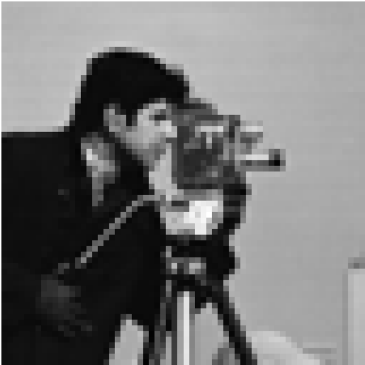
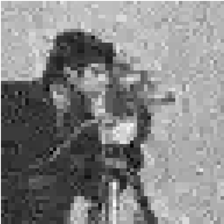
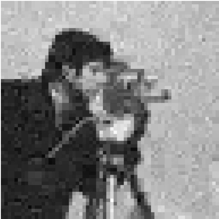
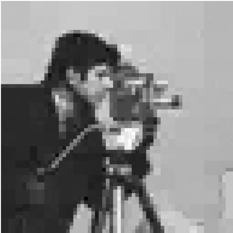
It is well known that 2D natural images are sparse in a wavelet basis. Their wavelet coefficients have a hierarchical tree structure, which is widely used for wavelet-based compression algorithms [21]. Figure 5 shows a widely used example image with size : cameraman. Each 2D wavelet coefficient of this image is connected to its parent coefficient and child coefficients, which forms the underlying hierarchical tree structure (which is a special case of graph sparsity). In our experiment, we choose Haar-wavelet to obtain its tree-structured sparsity wavelet coefficients. The projection matrix and noises are generated with the same method as that for 1D structured sparsity signals. OMP, Lasso and StructOMP are used to recover the wavelet coefficients from the random projection samples respectively. Then, the inverse wavelet transform is used to reconstruct the images with these recovered wavelet coefficients. Our task is to compare the recovery performance of the StructOMP to those of OMP and Lasso.
Figure 5 shows one example of the recovered results by different algorithms. It shows that StructOMP obtains the best recovered result. Figure 6 shows the recovery performance of the three algorithms, averaged over 100 random runs for each sample size. The StructOMP algorithm is better than both Lasso and OMP in this case. Since real image data are weakly sparse, the performance of standard OMP (without structured sparsity) is similar to that of Lasso.
7.3 Background Subtracted Images for Robust Surveillance
Background subtracted images are typical structure sparsity data in static video surveillance applications. They generally correspond to the foreground objects of interest. Unlike the whole scene, these images are not only spatially sparse but also inclined to cluster into groups, which correspond to different foreground objects. Thus, the StructOMP algorithm can obtain superior recovery from compressive sensing measurements that are received by a centralized server from multiple and randomly placed optical sensors. In this experiment, the testing video is downloaded from http://homepages.inf.ed.ac.uk/rbf/CAVIARDATA1/. The background subtracted images are obtained with the software [28]. One sample image frame is shown in Figure 7. The support set of 2D images is thus composed of several connected regions. Here, each pixel of the 2D background subtracted image is connected to four of its adjacent pixels, forming the underlying graph structure in graph sparsity. The results shown in Figure 7 demonstrate that the StructOMP outperforms both OMP and Lasso in recovery. We randomly choose 100 background subtracted images as test images. Figure 6 shows the recovery performance as a function of increasing sample sizes. It demonstrates again that StructOMP significantly outperforms OMP and Lasso in recovery performance on video data. Comparing to the image compression example in the previous section, the background subtracted images have a more clearly defined sparsity pattern where nonzero coefficients are generally distinct from zero (that is, stronger sparsity); this explains why Lasso performs better than the standard (unstructured) OMP on this particular data. The result is again consistent with our theory.


8 Discussion
This paper develops a theory for structured sparsity where prior knowledge allows us to prefer certain sparsity patterns to others. Some examples are presented to illustrate the concept. The general framework established in this paper includes the recently popularized group sparsity idea has a special case.
In structured sparsity, the complexity of learning is measured by the coding complexity instead of which determines the complexity in standard sparsity. Using this notation, a theory parallel to that of the standard sparsity is developed. The theory shows that if the coding length is small for a target coefficient vector , then the complexity of learning can be significantly smaller than the corresponding complexity in standard sparsity. Experimental results demonstrate that significant improvements can be obtained on some real problems that have natural structures.
The structured greedy algorithm presented in this paper is the first efficient algorithm proposed to handle the general structured sparsity learning. It is shown that the algorithm is effective under appropriate conditions. Future work include additional computationally efficient methods such as convex relaxation methods (e.g. regularization for standard sparsity, and group Lasso for strong group sparsity) and backward greedy strategies to improve the forward greedy method considered in this paper.
References
- [1] Francis R. Bach. Consistency of the group lasso and multiple kernel learning. JMLR, 9:1179–1225, 2008.
- [2] R. Baraniuk, V. Cevher, M. Duarte, and C. Hegde. Model based compressive sensing. 2008. preprint.
- [3] E. Berg, M. Schmidt, M. Friedlander, and K. Murphy. Group sparsity via linear-time projection. 2008. Preprint.
- [4] Iain Johnstone Bradley Efron, Trevor Hastie and Robert Tibshirani. Least angle regression. Annals of Statistics, 32:407–499, 2004.
- [5] Florentina Bunea, Alexandre B. Tsybakov, and Marten H. Wegkamp. Aggregation for Gaussian regression. Annals of Statistics, 35:1674–1697, 2007.
- [6] Emmanuel J. Candes and Terence Tao. Decoding by linear programming. IEEE Trans. on Information Theory, 51:4203–4215, 2005.
- [7] Thomas M. Cover and Joy A. Thomas. Elements of Information Theory. Wiley-Interscience, 1991.
- [8] L. Daudet. Sparse and structured decomposition of audio signals in overcomplete spaces. In International Conference on Digital Audio Effects, 2004.
- [9] D. Donoho. Compressed sensing. IEEE Transactions on Information Theory, 52:1289–1306, 2006.
- [10] D. Grimm, T. Netzer, and M. Schweighofer. A note on the representation of positive polynomials with structured sparsity. Arch. Math., 89:399–403, 2007.
- [11] L. He and L. Carin. Exploiting structure in wavelet-based bayesian compressive sensing. In Preprint, 2008.
- [12] L. He and L. Carin. Exploiting structure in compressive sensing with a jpeg basis. In Preprint, 2009.
- [13] Junzhou Huang and Tong Zhang. The benefit of group sparsity. Technical report, Rutgers University, January 2009. Available from http://arxiv.org/abs/0901.2962.
- [14] S. Ji, D. Dunson, and L. Carin. Multi-task compressive sensing. IEEE Transactions on Signal Processing, 2008. Accepted.
- [15] Vladimir Koltchinskii and Ming Yuan. Sparse recovery in large ensembles of kernel machines. In COLT’08, 2008.
- [16] M. Kowalski and B. Torresani. Structured sparsity: from mixed norms to structured shrinkage. In Workshop on Signal Processing with Adaptive Sparse Representations, 2009.
- [17] S. Mallat. In A Wavelet Tour of Signal Processing. Academic Press.
- [18] Yuval Nardi and Alessandro Rinaldo. On the asymptotic properties of the group lasso estimator for linear models. Electronic Journal of Statistics, 2:605–633, 2008.
- [19] G. Obozinski, M. J. Wainwright, and M. I. Jordan. Union support recovery in high-dimensional multivariate regression. Technical Report 761, UC Berkeley, 2008.
- [20] G. Pisier. The volume of convex bodies and banach space geometry. 1989. Cambridge University Press.
- [21] Jerome M. Shapiro. Embedded image coding using zerotrees of wavelet coefficients. IEEE Transactions on Signal Processing, 41:3445–3462, 1993.
- [22] Robert Tibshirani. Regression shrinkage and selection via the lasso. Journal of the Royal Statistical Society, 58:267–288, 1996.
- [23] J. Tropp and A. Gilbert. Signal recovery from random measurements via orthogonal matching pursuit. IEEE Transactions on Information Theory, 53(12):4655–4666, 2007.
- [24] D. Wipf and B. Rao. An empirical Bayesian strategy for solving the simultaneous sparse approximation problem. IEEE Transactions on Signal Processing, 55(7):3704–3716, 2007.
- [25] M. Yuan and Y. Lin. Model selection and estimation in regression with grouped variables. Journal of The Royal Statistical Society Series B, 68(1):49–67, 2006.
- [26] Tong Zhang. Adpative forward-backward greedy algorithm for learning sparse representations. Technical report, Rutgers Statistics Department, 2008. A short version appeared in NIPS 08.
- [27] P. Zhao, G. Rocha, and B. Yu. Grouped and hierarchical model selection through composite absolute penalties. The Annals of Statistics. to appear.
- [28] Z. Zivkovic and F. Heijden. Efficient adaptive density estimation per image pixel for the task of background subtraction. Pattern Recognition Letters, 27(7):773–780, 2006.
Appendix A Proof of Proposition 6.1
Lemma A.1
Consider a fixed vector , and a random vector with independent sub-Gaussian components: for all and , then :
Proof
Let ; then by assumption,
, which implies
that
.
Now let , we obtain the desired bound.
The following lemma is taken from [20]. Since the proof is simple, it is included for completeness.
Lemma A.2
Consider the unit sphere in (). Given any , there exists an -cover such that for all , with .
Proof Let be the unit ball in . Let be a maximal subset such that for all . By maximality, is an -cover of . Since the balls are disjoint and belong to , we have
Therefore,
which implies that .
Proof of Proposition 6.1
According to Lemma A.2, given , there exists a finite set with such that for all , and for all .
For each , Lemma A.1 implies that :
Taking union bound for all , we obtain with probability exceeding :
for all .
Let , then there exists such that . We have
Therefore
Let , and , we have
and thus
This simplifies to the desired bound.
Appendix B Proof of Theorem 6.1
We use the following lemma from [13].
Lemma B.1
Suppose is generated according to Theorem 6.1. For any fixed set with and , we have with probability exceeding :
| (5) |
for all .
Proof of Theorem 6.1
Since is a coding length, we have
where we let in the above derivation.
We can thus take the union bound over , which shows that with probability exceeding
the structured RIP in Equation (4) holds. Since
we obtain the desired bound.
Appendix C Proof of Theorem 6.2 and Theorem 6.3
Lemma C.1
Suppose that Assumption 6.1 is valid. For any fixed subset , we have with probability , such that , and , we have
Proof Let
be projection matrix to the subspaces generated by columns of .
Let , and , we have
Note that in the above derivation, we have used the fact that , and .
Now, by solving the above inequality, we obtain
The desired bound now follows easily from Proposition 6.1 and Lemma A.1, where we know that with probability ,
and with probability ,
We obtain the desired result by
substituting the above two estimates and simplify.
Lemma C.2
Suppose that Assumption 6.1 is valid. Then we have with probability , and :
Proof Note that for each , with probability , we obtain from Lemma C.1 that ,
Since , the result follows
from the union bound.
Lemma C.3
Consider a fixed subset . Given any , we have with probability :
Lemma C.4
Suppose that Assumption 6.1 is valid. Consider any fixed target . Then with probability exceeding , for all such that: , and for all , we have
where and . Moreover, if the coding scheme is sub-additive, then
Proof We obtain from the union bound of Lemma C.2 (with probability ) and Lemma C.3 (with probability ) that with probability :
This proves the first claim of the theorem.
The first claim with implies that
Since
,
we have
.
This implies the second claim.
Proof of Theorem 6.2
Proof of Theorem 6.3
Appendix D Proof of Theorem 6.4 and Theorem 6.5
The following lemma is an adaptation of a similar result in [26] on greedy algorithms for standard sparsity.
Lemma D.1
Suppose the coding scheme is sub-additive. Consider any , and a cover of by :
Let . Let . Then for all such that ,
and , we have
where as in (3), we define
Proof For all , achieves the minimum at (where is the vector of zeros except for the -th component, which is one). This implies that
for all . Therefore we have
Now, let be disjoint sets such that . The above inequality leads to the following derivation :
Note that we have used the fact that for all such that . By optimizing over , we obtain
This leads to the desired bound.
Proof of Theorem 6.4
Let
By Lemma D.1, we have at any step :
which implies that
Therefore at stopping, we have
This proves the theorem.
Proof of Theorem 6.5
For simplicity, let . For each , let be the largest such that
Let .
We prove by contradiction. Suppose that the theorem does not hold, then for all before stopping, we have .
Moreover, for each , Lemma D.1 (with ) implies that
Therefore we have
Now by summing over , we have
This is a contradiction because we know at stopping, we should have .
Appendix E Proof of Corollary 6.1
Given , we consider . We may assume that is achieved with . Note that by Lemma C.3, we have with probability :
This means the above inequality holds for all with probability . Now, by taking in Theorem 6.5, we obtain
where we have used the simple inequality when . Therefore,
This means that Theorem 6.5 can be applied to obtain the desired bound.