Spin Ice

Water ice is a fascinating strongly correlated condensed matter system, not least because it exhibits a seemingly violation of the third law of thermodynamics. In the early 1930s, a series of remarkable specific heat experiments by William Giauque and co-workers found that the limiting low-temperature state of the common (hexagonal) state of water ice, referred to as I_h, is characterized by a residual entropy, $S_{0}=0.82\pm 0.05$ Cal/deg$\cdot$mol, that differs from zero by a value far in excees of experimental errors [2, 3]. In a famous 1935 paper, Linus Pauling showed that, because of its configurational proton disorder, I_h possesses a finite entropy at zero temperature estimated as 0.81 Cal/deg$\cdot$mol [4], hence very close to the experimental value.

The ice problem is a classic example of how the separation of energy scales in an interacting system can leave some effective low energy degrees of freedom innoperative and ultimately frustrated in a system’s overall agenda in minimizing its energy at low temperature via local dynamical processes and over a finite, as opposed to infinite, amount of time. Here, the chemical binding energy of the water molecule is so strong, 221 kCal/mol, that its chemical structure is left essentially unaltered in the solid phase. Consequently, the ground state of water ice does not, or more precisely, dynamically cannot, minimize the electrostatic energy of a globally neutral ensemble of ${\rm O^{2-}}$ and ${\rm H^{+}}$ ions. Rather, in the hexagonal (“wurtzite”) and cubic (“sphalerite”) phases of ice [11], the O^2- ions form an open tetrahedral structure, whose $109$ degree angles accomodate almost perfectly that of the ${\rm H-O-H}$ bonds of an isolated H₂O molecule. In the wurtzite phase, the bond length between two distinct O^2- ions is $2.76$ Å, while the covalent ${\rm O-H}$ bond of a H₂O molecule is a much smaller $0.96$ Å. As the integrity of the molecular structure of H₂O is maintained in the solid phase, the minimum energy position of a H⁺ proton is not at the midpoint between two O^2- ions. Instead, there are two equivalent positions for a proton lying on an ${\rm O}-{\rm O}$ bond. With the four-fold oxygen co-ordination in the hexagonal wurtzite structure, there is in effect one proton per ${\rm O}-{\rm O}$ bond on average. The constraint imposed by the energetically robust ${\rm H_{2}O}$ structure therefore results in the two so-called Bernal-Fowler ice rules which govern what are acceptable low-energy proton configurations in the hexagonal wurtzite structure  [10]. The first ice rule states that there should only be one proton per ${\rm O}-{\rm O}$ on average. The second rule states that, in order for ice to consist of a hydrogen-bonded solid of water molecules, for each O^2- ions, two H⁺ protons must be in a “near-to-O^2-” position, and two protrons must be in a “far position” (see Fig. 1). From a solely electrostatic point of view, the protons would like to be as far apart as possible. The ice rules, implemented via the unaltered integrity of the H₂O water molecule, render the proton-proton interaction an effectively low-energy part of the problem, and frustrates it.

The ice rules were put forward by Bernal and Fowler in 1933 [10]. At that time, X-ray diffraction could only determine the lattice structure for the oxygen atoms. According to the first ice rule, Bernal and Fowler argued that the hydrogens must lie along the direct oxygen-oxygen line of contact (bond) between two H₂O molecules. They proposed a regular crystalline proton structure, presumably expecting that this would be the case. However, around the same time, Giauque and co-workers had already obtained compelling evidence for a residual zero point entropy in water ice [2]. This led Pauling to his proposal, published in 1935, that the open tetrahedral structure of ice leads to many equivalent ways of satisfying the Bernal-Fowler ice rules, and hence to an extensive entropy [4].

Pauling put forward an elegant argument to estimate the configurational proton entropy. The argument goes as follows. First consider one mole of ice containing $N_{0}$ ${\rm O^{2-}}$ ions and, therefore, $2N_{0}$ ${\rm O-O}$ bonds for the hexagonal structure of ice in which no two proton are on any given ${\rm O-O}$ bond. That is, all bonds are taken to obey the first Bernal-Fowler ice rule. Each ${\rm O-O}$ bond can be taken as having two possible positions for a proton. This gives $2^{(2N_{0})}$ possible proton configurations for the whole system. Out of the 16 possible configurations associated with each oxygen, ten are energetically unfavourable: the ${\rm OH_{4}^{2+}}$ configuration, the 4 ${\rm OH_{3}^{+}}$ configurations, the 4 ${\rm OH^{-}}$ configurations and the ${\rm O^{2-}}$ configuration. This leaves six configurations that satisfy the Bernal-Fowler rules as the allowed local proton configurations around each oxygen ion. An upper bound on the number of ground state configurations, $\Omega_{0}$, can therefore be estimated by reducing the above $2^{2N_{0}}$ configurations by a simple $6/16$ deflation weight factor for each oxygen ion. This gives $\Omega_{0}\leq 2^{2N_{0}}(6/16)^{N_{0}}=(3/2)^{N_{0}}$. The corresponding configurational entropy, $S_{0}=k_{\rm B}\ln(\Omega_{0})=N_{0}k_{\rm B}\ln(3/2)=0.81$ Cal/deg$\cdot$mol, is in excellent agreement with the residual entropy of $0.82\pm 0.05$ Cal/deg$\cdot$mol determined by Giauque and Stout [3]. Pauling’s calculation neglects the global constraint on the number of protons as well as the local constraints coming from closed loops on the wurtzite lattice. Nevertheless, Pauling’s estimate has been shown to be accurate to $1-2\%$ [12].

In a 1956 paper [13], Anderson investigated the problems of cation ordering in the so-called inverse spinel materials and that of magnetic ordering in normal spinels. To a first approximation, both of these problems map onto the problem of an Ising model with antiferromagnetic nearest-neighbor exchange interaction on the B-site of the spinel lattice. This lattice is structurally identical to the pyrochlore lattice shown in Fig. 2. For a discussion of magnetic ordering in spinels, see the Chapter by Takagi in this book.

Consider first the problem of cation ordering in the inverse spinel. The associated minimum energy problem consists in placing $+$ and $-$ signs on the pyrochlore lattice (see Fig. 2) in a ratio 1:1 such that the number of $+/-$ pairs is maximized. This condition is satisfied with two $+$ and two $-$ signs for each tetrahedron. The center of the tetrahedra in the spinel lattice are arranged with respect to each other on the same lattice at the oxygen ions in the cubic phase of water ice (I_c). As shown in Fig. 2, the spinel latice and, equivalently, the pyrochlore lattice, consists of alternating “upward” and “downward” tetrahedra. Consequently, the problem of $+$ and $-$ charge organization problem maps onto an ice rule problem if a $+$ sign corresponds to a “proton near” on an upward tetrahedron and a “proton far” on a downward tetrahedron, and vice-versa for a $-$ sign. Neglecting the same constraints that Pauling neglected for the water ice problem, the problem of cation ordering in inverse spinels therefore maps onto an ice-like problem, and is therefore characterized by a Pauling zero point entropy [13]. The problem of cation ordering is also manifestly the same as that of an antiferromagnetic Ising model on the pyrochlore lattice, where $+$ represents a spin up and $-$ represents a spin down. It is interesting to note that in the context of an antiferromagnetic Ising model on the pyrochlore lattice, Anderson’s model was the second example of what would now be referred to as a frustrated antiferromagnet, the first one being the problem of the Ising antiferromagnet on the triangular lattice studied by Wannier in 1950  [1].

Anderson’s model is an important paradigm for frustrated magnetic systems of interacting spins that reside on the sites of a lattice of corner-shared triangles or tetrahedra, as occurs in kagome, garnet and pyrochlore lattices. Yet, there are no known realizations of Anderson’s Ising antiferromagnet on the pyrochlore lattice. The reason is that the pyrochlore lattice has a cubic symmetry, and there is no energetic reason permitted by symmetry that would favor a unique global $\hat{z}$ Ising direction to the detriment of another global direction. However, a system of antiferromagnetically coupled isotropic Heisenberg spins on the pyrochlore lattice is realistic. This problem was the topic of an important 1979 paper [14]. In that work, Villain anticipated the failure of the classical Heisenberg pyrochlore antiferromagnet to develop long range order down to zero temperature [15, 16] and coined the name collective paramagnet to this system $-$ a terminology that one may want to ascribe to the classical variant of the more modern terminology of spin liquid used in quantum spin systems. Because they lack the intrinsic propensity to develop classical long range magnetic order, antiferromagnetic materials with Heisenberg spins that reside on a pyrochlore lattice are expected to be excellent candidates to display exotic quantum mechanical ground states. It is the anticipation of the observation of interesting magnetic and thermodynamic behaviors in the broad familly of magnetic pyrochlore oxide materials, of generic formula A₂B₂O₇, that led at the end of the 1980’s to the rapid rise of experimental and theoretical efforts devoted to the study of these systems [17, 18]. It is also this general scientific endeavour that led to the discovery of spin ice [5, 6, 7], a novel class of frustrated ferromagnet Ising systems, close analogues of both water ice and the cation ordering in spinels. This discovery also led to the rebirth of a disguised variant of Anderson’s antiferromagnetic Ising model [13] on the pyrochlore lattice.

Before reviewing the discovery of spin ice materials and the spin ice problematic, we first briefly discuss some general aspects of the pyrochlore oxides, the broader class of materials to which spin ices belong. We also review the elementary background behind the origin of the magnetism in the rare earth ions involved in spin ices, how they acquire their strong Ising nature, and what the predominant interactions between the magnetic ions are.

The A₂B₂O₇ magnetic pyrochlore oxides form a broad familly of materials that exhibit a wide range of interesting thermodynamic and magnetic phenomena, a number of which are still poorly understood [17, 18]. Here, both the trivalent A³⁺ ion (A is a rare earth element such as Gd, Tb, Dy, Ho, etc, or Y) and the tetravalent B⁴⁺ ion (B=Ti, Sn, Mo, Mn) reside on two independent and interpenetrating pyrochlore sublattices. Figure 2 shows only one of those two sublattices, say the A sublattice. In A₂B₂O₇, one can have either the A or the B sublattice occupied by a magnetic ion, as in Tb₂Ti₂O₇  [19] and Y₂Mo₂O₇  [20], respectively, or both sites can be occupied by a magnetic ion such as in Tb₂Mo₂O₇  [21]. As discussed by Villain already thirty years ago [14], the pyrochlore lattice is highly frustrated when the ions carry an isotropic Heisenberg spin and interacts with nearest neighbors via an antiferromagnetic exchange coupling. The pyrochlore oxides can be metallic (e.g. Nd₂Mo₂O₇, which displays an interesting anomalous Hall effect [22]) or they can be insulating, as is the case for the A₂Ti₂O₇ and A₂Sn₂O₇ series [17, 18]. In this chapter, we shall restrict ouselves to the insulating A₂Ti₂O₇ and A₂Sn₂O₇ series with Dy and Ho as magnetic ion A; Ti⁴⁺ and Sn⁴⁺ are non-magnetic. That is, we are dealing with only one magnetic pyrochlore sublattice, the A sublattice, in A₂B₂O₇, which we henceforth simply refer to “the pyrochlore lattice”. Neglecting spin-spin interactions [23], the Tb³⁺ ion in Tb₂Ti₂O₇ and Tb₂Sn₂O₇ would also be described as an Ising spin at sufficiently low temperatures [24, 25]. However, interactions make the strictly Ising model description of these two materials invalid [23].

The pyrochlore lattice can be conveniently described as a face-centered cubic (FCC) lattice with a primitive (“upward”, or “downward”) tetrahedron basis cell of four sites (see Fig. 2). The pyrochlore lattice possesses a trigonal (threefold rotational) symmetry with respect to any of the four equivalent $\langle 111\rangle$ cubic lattice directions (i.e. the diagonals of the cubic cell in Fig. 2). For each of the four sites in the tetrahedron unit cell, it will prove convenient to use as local $\hat{z}_{i}$ axis of spin quantization the specific $[111]$ cube diagonal that passes through a given site $i$ and the middle of the opposite triangular face (see. Fig. 2).

One should note that common water ice at atmospheric pressure, ice I_h, has a hexagonal structure while the magnetic pyrochlore lattice has a cubic symmetry. Strictly speaking, the Ising pyrochlore problem is equivalent to cubic ice, $I_{\rm c}$, and not the hexagonal I_h phase. However, this does not modify the “ice-rule” analogy (or mapping) or the close connection between the orientation of the magnetic moments in spin ice and the local proton coordination in water ice.

The spin-orbit interaction is large in rare-earth ions and the total angular momentum, ${\bf J}={\bf L}+{\bf S}$, can be taken as a good quantum number. For a given ion, one can apply Hund’s rules to determine the isolated (vacuum) electronic ground state. For example, Tb has an electronic configuration [Xe]4f⁹6s² and Tb³⁺ has [Xe]4f⁸ as electronic ground state configuration. Following Hund’s rules, one finds that L=3 and S=3, hence J=6 for Tb³⁺ and the spectroscopic notation for the ground multiplet is ⁷f₆. Similarly, one finds J=8 for Ho₂Ti₂O₇ and J=15/2 for Dy₂Ti₂O₇. Electrostatic and covalent bonding effects, which originate from the crystalline environment, lead to a lifting of the otherwise free ion ground state (2J+1)-fold electronic degeneracy. This is the so-called crystal field effect. The theoretical description of crystal field effects going beyond the simple Coulomb point charge description of the charges surrounding a rare earth ion, and which includes covalency effects and admixing between electronic multiplets, is a rather technical problem which we shall not discuss here. In the forthcoming discussion, we will merely assume that the single-ion crystal field energy levels (of the non-interacting ions) have been “suitably” determined. This can be done, for example, via experimental spectroscopic methods (e.g. optical spectroscopy, inelastic neutron scattering, etc). Such a spectroscopic approach allows to determine the transition frequencies between crystal-field levels and their intensities which can then be described by a so-called crystal field Hamiltonian, ${\cal H}_{\rm cf}$ (see for example Refs. [24, 25, 26]). We shall return to this point shortly. Ideally, one would like to make sure that the energy levels so-determined are not strongly “dressed” (i.e. affected, or renormalized) by inter-ion interactions described by ${\cal H}_{\rm int}$. This can sometimes be done by considering a highly magnetically diluted variant of the system of interest [25]. This leads us to introduce the Hamiltonian, ${\cal H}$, needed to describe the minimal physics at stake:

$${\cal H}={\cal H}_{\rm cf}+{\cal H}_{\rm Z}+{\cal H}_{\rm int}\;.$$

(1)

Here ${\cal H}_{\rm cf}$ is the crystal-field Hamiltonian responsible for the lifting of the degeneracy of the otherwise free single-ion electronic ground state. Its energy eigenstates are the above crystal-field energy levels. As a first approximation, one can express ${\cal H}_{\rm cf}$ in terms of polynomial functions of the J_i,z and ${\rm J}_{i,\pm}={\rm J}_{i,x}\pm\imath{\rm J}_{i,y}$ components of the angular momentum operator ${\bf J}$. For the local symmetry of the rare-earth ions at the A site in A₂B₂O₇, one writes ${\cal H}_{\rm cf}$ [24, 25, 26] as

$${\cal H}_{\rm cf}=\sum_{i}\sum_{l,m}B_{l}^{m}O_{l}^{m}({\bf J}_{i})\;,$$

(2)

where $B_{l}^{m}$ are the crystal field coefficients and $O_{l}^{m}({\bf J}_{i})$ are the equivalent crystal field operators. Spectroscopic measurements allow to determine the $B_{l}^{m}$ via a fitting procedure of the energy levels with further constraints from the observed transition intensities [24, 26]. Because of the Wigner-Eckart theorem, $l\leq 6$ for L=3 4f elements. For example, $O_{2}^{0}=3{\rm J}_{z}^{2}-{\rm J}({\rm J}+1)$, $O_{4}^{0}=35{\rm J}_{z}^{4}-(30{\rm J}({\rm J}+1)-25){\rm J}_{z}^{2}+3{\rm J}^{2}({\rm J}+1)-6{\rm J}({\rm J}+1))$ and $O_{4}^{\pm 3}=c_{\pm}[{\rm J}_{z},{\rm J}_{+}^{3}\pm{\rm J}_{-}^{3}]_{+}$ with $[A,B]_{+}=(AB+BA)/2$, $c_{+}=1/2$ and $c_{-}=-\imath/2$ (see Refs. [27, 28, 29]).

In Eq. 1 ${\cal H}_{\rm Z}=-g_{\rm L}\mu_{\rm B}\sum_{i}{\bf J}_{i}\cdot\vec{B}$ is the Zeeman energy describing the interactions of the rare earth magnetic ions with the magnetic field $\vec{B}$; $g_{\rm L}$ is the Landé factor and $\mu_{\rm B}$ is the Bohr magneton. Finally, ${\cal H}_{\rm int}$ describes the interactions between the ions. We consider the following form for ${\cal H}_{\rm int}$:

$${\cal H}_{\rm int}=-\frac{1}{2}\sum_{(i,j)}{\cal J}_{ij}\,{\bf J}_{i}\cdot{\bf J}_{j}+\left(\frac{\mu_{0}}{4\pi}\right)\frac{(g_{\rm L}\mu_{\bf B})^{2}}{{2{r_{\rm nn}}^{3}}}\sum_{(i,j)}\frac{({\bf J}_{i}\cdot{\bf J}_{j}-3{\bf J}_{i}\cdot\hat{r}_{ij}\hat{r}_{ij}\cdot{\bf J}_{j})}{(r_{ij}/r_{\rm nn})^{3}}\;,$$

(3)

where $\vec{r}_{j}-\vec{r}_{i}=r_{ij}\hat{r}_{ij}$ with $\vec{r}_{i}$ the position of ion $i$. Here ${\cal J}_{ij}$ is the microscopic quantum mechanical exchange constant between ions $i$ and $j$. We use the convention that ${\cal J}_{ij}<0$ is antiferromagnetic and ${\cal J}_{ij}>0$ is ferromagnetic. Note that in Eq. (3), the two sums are carried over all ions $i$ and $j$, hence there is double-counting, and this is why there is a pre-factor $1/2$ in front of each sum. The first term “originates” from the interactions between the “real” electronic spins, $\vec{S}_{i}$ and $\vec{S}_{j}$. For simplicity, we only consider here an effective isotropic “exchange” between the total angular momenta ${\rm J}_{i}$ and ${\rm J}_{j}$ with exchange interactions ${\cal J}_{ij}$. Such description has proven adequate to describe the physics of spin ice materials [30, 31, 32, 33]. The four distinct types of symmetry-allowed anisotropic exchange interactions on the pyrochlore lattice are described in Refs. [34, 35] The second term is the long range magnetostatic dipole-dipole interaction with $r_{\rm nn}$ the distance between nearest neighbors. The pyrochlore oxides have a conventional cubic unit cell of size $a\sim 10\AA$ with 16 ions (i.e. 4 “upward” or “downward’ primitive tetrahedron basis cells, see Fig. 2) per conventional cubic unit cell and $r_{\rm nn}=(a\sqrt{2})/4$. We now discuss the relative energy scales set by ${\cal H}_{\rm cf}$, ${\cal H}_{\rm Z}$ and ${\cal H}_{\rm int}$.

By far, for the (Ho,Dy)₂(Ti,Sn)₂O₇ materials, which we will show later are spin ices, ${\cal H}_{\rm cf}$ sets the largest energy scale in the problem. In these four materials, the spectrum of ${\cal H}_{\rm cf}$ consists of a ground state doublet separated by an energy gap, $\Delta$, of typically $\Delta\sim 300$ K, to the first excited state. The Landé factor $g_{\rm L}$ of Ho³⁺ and Dy³⁺ is 5/4 and 4/3, respectively, and $\mu_{\rm B}=9.27\times 10^{-24}$ J/T $\approx 0.671$ K/T in $H_{\rm Z}$. In other words, even for a field of 20 T, which is about the largest field accessible via commercial in-house magnets, the Zeeman energy scale is of the order of 10 K, hence much smaller than $\Delta$. Consequently, when calculating the properties of (Ho,Dy)₂(Ti,Sn)₂O₇ at temperatures $T<~10$ K and in magnetic fields less than 20 T or so, on can safely consider only the magnetic crystal-field ground state doublet of Ho³⁺ and Dy³⁺ and ignore the susceptibility contributions from the excited states as well as the van Vleck susceptibility. The interaction part, ${\cal H}_{\rm int}$, deserves particular attention. In insulating magnetic rare earth materials, the unfilled 4f spin-carrying orbitals of the rare earth ion are shielded by 5s and 5p orbitals and the 4f orbital overlap between the rare earth ions and between rare earths and O^2- is therefore small. Consequently, the effective ${\cal J}_{ij}$ exchange coupling between rare earth ions is much smaller in insulating rare earth oxides compared to that of transition metal oxides. For example, a typical value for ${\cal J}_{ij}$ for nearest neighbors, ${\cal J}$, is ${\cal J}\sim 66$ mK in Dy₂Ti₂O₇  [30, 33]. We can also estimate the dipolar energy scale, ${\cal D}\equiv\mu_{0}(g_{\rm L}\mu_{\rm B})^{2}/(4\pi{r_{\rm nn}}^{3})$. Plugging in a value $r_{\rm nn}\sim 3.5\AA$ and $g_{\rm L}=4/3$, we get ${\cal D}\sim 25$ mK  [30, 33]. Comparing ${\cal J}$ and ${\cal D}$ with $\Delta\sim 300$ K, one sees that the interaction part ${\cal H}_{\rm int}$ of the full Hamiltonian ${\cal H}$ is very small compared to the crystal-field part, ${\cal H}_{\rm cf}$ [36]. In practice, this means that the independent/non-interacting single-ion crystal-field eigenstates of ${\cal H}_{\rm cf}$ form a very convenient basis to describe the Hilbert space of interacting Dy³⁺ and Ho³⁺ ions in (Ho,Dy)₂(Ti,Sn)₂O₇. In particular, since the scale of ${\cal H}_{\rm int}$ is so small compared to $\Delta$, one can, for all practical purposes, neglect all the excited states of ${\cal H}_{\rm cf}$ and work with a reduced Hilbert space solely spanned by the two degenerate states of the ground doublet for each magnetic sites. In such a problem, where the high-energy sector of the theory is so well separated from the low-energy sector, it is convenient to introduce a so-called effective Hamiltonian, ${\cal H}_{\rm eff}$, that operates only within the low-energy sector. The Chapter by Mila and Schmidt in this book describes the general methodology as to how to derive a ${\cal H}_{\rm eff}$ for a given interacting system where there are well separated “reference” energy sectors. For the spin ices, the lowest order of the perturbation theory which defines ${\cal H}_{\rm eff}$ is amply sufficient; i.e.

$\displaystyle{\cal H}_{\rm eff}$

$\displaystyle\approx$

$\displaystyle P{\cal H}_{\rm int}P$

(4)

with $P$, the projector in the low-energy sector, defined as

$$P=\sum_{\{k\}}|\Phi_{0,\{k\}}\rangle\langle\Phi_{0,\{k\}}|$$

(5)

where

$$|\Phi_{0,\{k\}}\rangle=\prod_{i=1}^{N}|\phi_{i,0}^{(k_{i})}\rangle\;.$$

(6)

Here $\phi_{i,0}^{(k_{i})}$ is the $k_{i}^{\rm th}$ state of the single-ion crystal-field ground doublet of rare earth ion $i$. Since ${\cal H}_{\rm int}$ is a pairwise Hamiltonian, ${\cal H}_{\rm eff}$ is, to lowest order and given by Eq. (4), also a pairwise effective Hamiltonian. One can then determine ${\cal H}_{\rm eff}$ by considering two ions each in one of the two states, $|\phi_{i,0}^{(k_{i}=+)}\rangle$ and $|\phi_{i,0}^{(k_{i}=-)}\rangle$, of their respective crystal-field ground doublet. Hence, the effective Hamiltonian ${\cal H}_{\rm eff}$ is a $4\times 4$ matrix. At this point, we need to return to the crystal-field problem and discuss the nature of the non-interacting $|\phi_{i,0}^{(k_{i}=\pm)}\rangle$ states that make each of the single-ion ground doublet.

From inelastic neutron measurements, it is found that $|\phi_{i,0}^{(k_{i}=+)}\rangle$ and $|\phi_{i,0}^{(k_{i}=-)}\rangle$ for Ho₂Ti₂O₇ are $|\phi_{i,0}^{(k_{i}=\pm)}\rangle\approx|{\rm J}=8,m_{\rm J}=\pm 8\rangle$, with negligible contributions from other $|{\rm J}=8,m_{\rm J}\rangle$ components. By rescaling the crystal field parameters determined for Ho₂Ti₂O₇ one can determine the crystal field parameters for Dy₂Ti₂O₇ [24]. One finds for the latter material $|\phi_{i,0}^{(k_{i}=\pm)}\rangle\approx|{\rm J}=15/2,m_{\rm J}=\pm 15/2\rangle$ with again negligible weight from other $|{\rm J}=15/2,m_{\rm J}\rangle$ components [24]. It is important to recall the above discussion about the choice of the $\hat{z}_{i}$ quantization direction. Here, the magnetic quantum number $m_{\rm J}$ eigenstate of ${\rm J}_{z}$ refers to the component of ${\bf J}_{i}$ along the local $\hat{z}_{i}$ direction that points along one of the four cubic $\langle 111\rangle$ directions. Calculating the matrix elements of $P{\cal H}_{\rm int}P$, one finds that, for both Ho₂Ti₂O₇ and Dy₂Ti₂O₇, the only significant matrix elements are $\langle\phi_{i,0}^{(k_{i}=\pm)}|{\rm J}_{z}|\phi_{i,0}^{(k_{i}=\pm)}\rangle\approx\pm{\rm J}$. The physical meaning is simple. In both Ho₂Ti₂O₇ and Dy₂Ti₂O₇, the magnetic moment can, for all practical purposes, only point parallel or antiparallel to the local $[111]$ direction; we are deadling with a local $\langle 111\rangle$ Ising model!

It is useful to write down the set of local $\hat{z}_{i}$ quantization axis (i.e. $\hat{z}_{i}\parallel\langle 111\rangle$ axis). We take $\hat{z}_{1}=\frac{1}{\sqrt{3}}(\hat{x}+\hat{y}+\hat{z})$, $\hat{z}_{2}=\frac{1}{\sqrt{3}}(-\hat{x}-\hat{y}+\hat{z})$, $\hat{z}_{3}=\frac{1}{\sqrt{3}}(-\hat{x}+\hat{y}-\hat{z})$ and $\hat{z}_{4}=\frac{1}{\sqrt{3}}(\hat{x}-\hat{y}-\hat{z})$, with $\hat{z}_{\mu}\cdot\hat{z}_{\nu}=-1/3$ for $\mu\neq\nu$. To proceed formally, one could re-express the above $4\times 4$ matrix representing ${\cal H}_{\rm eff}$ in terms of tensor products of Pauli matrices, $\sigma_{i}^{\alpha_{i}}\otimes\sigma_{j}^{\beta_{j}}$ where we are here using a local orthogonal $\{x_{i},y_{i},z_{i}\}$ frame [23], where $\alpha_{i}=x_{i},y_{i},z_{i}$. Had we kept the full $|{\rm J},m_{\rm J}\rangle$ decomposition of $|\phi_{i,0}^{(k_{i}=\pm)}\rangle$, one would have found that the coefficient of the $\sigma_{i}^{z_{i}}\sigma_{j}^{z_{j}}$ term has by far the largest coefficient in ${\cal H}_{\rm eff}$. We thus end up with a classical model with Ising spins pointing parallel or antiparallel to their local $[111]$ direction.

Alternatively, one could have proceeded much more straightforwardly and simply replace

$${\bf J}_{i}\rightarrow|\langle{\rm J}_{z}\rangle|\sigma_{i}^{z}\hat{z}_{i}$$

(7)

right at the outset, and use $|\langle{\rm J}_{z}\rangle|\approx 8$ for Ho₂Ti₂O₇ and $|\langle{\rm J}_{z}\rangle|\approx 15/2$ for Dy₂Ti₂O₇. Indeed, this is what was implicitely done in most previous numerical studies of dipolar spin ice [7, 30, 31, 32, 37, 38]. Since there are no other components $\sigma_{i}^{\alpha_{i}}$ with $\alpha_{i}\neq z_{i}$ that do not commute among themselves left in ${\cal H}_{\rm eff}$, we have a strictly classical Ising model for $H_{\rm eff}$. One can therefore work in the basis of eigenstates of $\sigma_{i}^{z_{i}}$ and, henceforth, we merely treat $\sigma_{i}^{z_{i}}=\pm 1$ as a classical variable. Admitedly, the discussion here leading to ${\cal H}_{\rm eff}$ as a classical Ising model for the Dy-based and Ho-based oxyde pyrochlores is rather academic. However, as mentioned earlier in Section 0.3.1 it is not so for Tb₂Ti₂O₇ [19] and Tb₂Sn₂O₇ [39]. Indeed, for these two materials, the energy gap separating the ground doublet and the excited doublet is not so large compared to the exchange and dipole-dipole interactions. In that case, higher order terms in the perturbation expansion leading to ${\cal H}_{\rm eff}$ must be retained (again, see the chapter by Mila and Schmidt) in order to derive a proper quantum theory of this material, as was recently done for a simple model of Tb₂Ti₂O₇ [23].

Returning to ${\cal H}_{\rm int}$ above, and writing ${\rm J}_{i}\rightarrow|\langle{\rm J}_{z}\rangle|\sigma_{i}^{z}\hat{z}_{i}$, we arrive at our effective classical $\langle 111\rangle$ pyrochlore Ising model

$${\cal H}_{\rm DSM}=-\frac{1}{2}\sum_{(i,j)}J_{ij}\,(\hat{z}_{i}\cdot\hat{z}_{j})\,\sigma_{i}^{z_{i}}\sigma_{j}^{z_{j}}\;+\;\frac{D}{2}\sum_{(i,j)}\frac{(\hat{z}_{i}\cdot\hat{z}_{j}-3\hat{z}_{i}\cdot\hat{r}_{ij}\hat{r}_{ij}\cdot\hat{z}_{j})}{(r_{ij}/r_{\rm nn})^{3}}\,\sigma_{i}^{z_{i}}\sigma_{j}^{z_{j}}\;,$$

(8)

which we shall henceforth refer to as the “dipolar spin ice model” (DSM). Here we have written $J_{ij}={\cal J}_{ij}\langle{\rm J}_{z}\rangle^{2}$ and $D=\mu_{0}(g_{\rm L}\mu_{\rm B}\langle{\rm J}_{z}\rangle)^{2}/(4\pi{r_{\rm nn}}^{3})$. Note that the variables $\sigma_{i}^{z}=\pm 1$ have become simple labels indicating whether the $z_{i}$-component of ${\bf J}_{i}$ points “in” or “out” of a primitive tetrahedron unit cell characterized by the above set $\{\hat{z}_{1},\hat{z}_{2},\hat{z}_{3},\hat{z}_{4}\}$ (see Fig. 2). Having established that the magnetic Dy³⁺ and Ho³⁺ ions in Dy₂Ti₂O₇ and Ho₂Ti₂O₇ should be described by effective classical Ising spins at temperatures much lower than the lowest crystal field gap $\Delta$, we can now proceed to discuss the experimental behavior of these two materials, and how the spin ice phenomenology arises.

In a 1997 paper, Harris, Bramwell and collaborators reported the results of a neutron scattering study of Ho₂Ti₂O₇ [5]. They found that, in zero applied magnetic field, no evidence of a transition to long range order could be detected down to 0.35 K via neutron scattering, while muon spin relaxation results could rule out a transition down to 0.05 K [6]. The most surprising part of those results was that the Curie-Weiss temperature, $\theta_{\rm CW}$, was found to be positive with $\theta_{\rm CW}\approx+1.9$ K, hence indicating overall ferromagnetic interactions. Naively, one would have expected such a three-dimensional cubic system with ferromagnetic interactions to develop long range order at a critical temperature of the same order of magnitude as $\theta_{\rm CW}$. It was also found that the magnetic field dependence of the neutron scattering intensity depends on the protocol followed to magnetize the sample [40]. In other words, the system displayed a history dependence reminiscent of what is observed in random spin glasses [41], although no significant random disorder is present in Ho₂Ti₂O₇.

The authors of Refs. [5, 6] proposed that the strong local $[111]$ Ising anisotropy of Ho³⁺ in Ho₂Ti₂O₇ frustrates the development of ferromagnetic order. They considered a simple model of ferromagnetically coupled $\langle 111\rangle$ Ising spins on the pyrochlore lattice [42]. By doing so, they established the connection between their model and that of Pauling’s model for the problem of proton disorder in water ice, hence coining the name spin ice model to their model (see Fig. 1). For clarity sake, and since we shall discuss below the important role that long range dipole-dipole interactions play in spin ice materials, we relabel Harris et al.’s model as nearest-neighbor spin ice model, in order to distinguish it from the dipolar spin ice model (DSM) of Eq. (8). We discuss in the next section this nearest-neighbor spin ice model and show that it has the same residual entropy as water ice.

The first compelling thermodynamic evidence for the existence of a spin ice state in Ising pyrochlore systems was obtained via measurements of the magnetic specific heat, $C(T)$, on Dy₂Ti₂O₇ [7]. This material with magnetic Dy³⁺ is, as Ho₂Ti₂O₇, characterized by a strongly Ising-like ground state doublet that is separated by a large energy of approximately 300 K from the excited doublet. The temperature dependence of $C(T)$ is shown in the upper panel of Fig. 3. To determine the residual magnetic entropy of Dy₂Ti₂O₇, Ramirez and co-workers followed an approach similar to the one that Giauque and colleagues used to determine the entropy of water ice [2, 3].

In general, one can only measure the change of entropy between two temperatures. Giauque and collaborators calculated the entropy change of water between 10 K and the gas phase of H₂O by integrating the specific heat divided by temperature, $C(T)/T$, adding to it the latent heat at the melting and vaporization transitions. They then compared this value with the absolute value expected for the entropy calculated for an ideal (non-interacting) gas phase using inputs from spectroscopic measurements which allowed to determine the rotational and vibrational energy spectrum, hence the roto-vibrational entropy, and adding to it the translational entropy of an ideal gas given by the Sackur-Tetrode equation. The difference between the measured value and the theoretically expected value gave the residual entropy of water ice, whose origin was explained by Pauling [4].

Ramirez et al. measured the magnetic specific heat of a powder sample of Dy₂Ti₂O₇ between $T_{1}$=300 mK, “deep” inside the frozen ice regime, and $T_{2}$=10 K, in the paramagnetic regime, where the expected entropy per mole should be $R\ln(2)$ for a two-state system (${R}=N_{0}k_{\rm B}$ is the gas molar constant and $N_{0}$ is the Avogadro number).

The entropy change between $T_{1}$ and $T_{2}$, $\Delta S_{1,2}$, was found by integrating $C(T)/T$ between these two temperatures:

$$\Delta S_{1,2}=S(T_{2})-S(T_{1})=\int_{T_{1}}^{T_{2}}\frac{C(T)}{T}\,dT.$$

(13)

The lower panel of Fig. 3 shows that the magnetic entropy recovered is approximately 3.9 Jmol^-1K^-1, a value quite a bit smaller than R$\ln(2)\approx$ 5.76 Jmol^-1K^-1. The difference, 1.86 Jmol^-1K^-1 is fairly close to the above Pauling-like estimate for the entropy associated with the extensive degeneracy of ice: $(R/2)\ln(3/2)=1.68$ Jmol^-1K^-1, consistent with the existence of an ice-rule obeying spin ice state in Dy₂Ti₂O₇. More recent measurements [44] on single crystals of Dy₂Ti₂O₇ have found a specific heat below 1.5 K that differs quantitatively fairly significantly from that of Ref. [7], ultimately giving a much better agreement between the experimentally determined residual entropy of the material and Pauling’s value.

As discussed above, Ho₂Ti₂O₇ was the first material proposed as a spin ice system. It turns out that Ho₂Ti₂O₇ is less convenient to perform low temperature specific heat measurements than Dy₂Ti₂O₇. The origin of this difficulty stems from the unusually large hyperfine interaction between the nuclear and electronic spins of Ho³⁺. This interaction leads to a Schottky anomaly in the specific heat at a temperature $T\sim 0.3$ K which significantly obscures the otherwise purely electronic broad specific heat feature arising from the formation of the ice-rule obeying low-energy manifold [45]. Once the nuclear contribution to the specific heat has been subtracted, the exposed electronic contribution and the consequential residual Pauling entropy of the spin ice state in Ho₂Ti₂O₇ can be revealed [31, 46].

In summary, the Ho₂Ti₂O₇ and Dy₂Ti₂O₇ possess a residual low-temperature entropy compatible with that estimated on the basis of a Pauling argument applied to the ferromagnetic nearest-neighbor $\langle 111\rangle$ Ising model on the pyrochlore lattice. The related Ho₂Sn₂O₇ [47] and Dy₂Sn₂O₇ [48] are also spin ice systems.

In Section 0.3.4, we invoked a simple nearest-neighbor ferromagnetic $\langle 111\rangle$ Ising model to rationalize the spin ice phenomenology in real materials. Yet, it was argued in Section 0.3.2 that magnetic dipole-dipole interactions are often of sizeable strength in rare-earth magnetic systems. In the case of Dy₂Ti₂O₇ and Ho₂Ti₂O₇, the value of $D=\mu_{0}(g_{\rm L}\mu_{\rm B}\langle{\rm J}_{z}\rangle)^{2}/(4\pi{r_{\rm nn}}^{3})$ is estimated at $D\sim 1.4$ K [30, 37, 38], which is comparable to the experimentally measured Curie-Weiss temperature $\theta_{\rm CW}$ in these materials. Even if one was assuming that the nearest-neighbor exchange $J\sim\theta_{\rm CW}\sim 1$ K, one is still in a regime where the dipolar interactions are comparable in magnitude to the nearest-neighbor exchange interactions [7, 30, 37]. This observation raises a paradox. The existence of a ground state with extensive degeneracy should in principle results from the underconstraints that the Hamiltonian imposes on the spin configurations that minimize the classical ground state energy [16]. Consider the dipolar interactions in Eq. (8). First of all, they are rather complicated as they couple spin and space directions via the $(\hat{z}_{i}\cdot\hat{r}_{ij})(\hat{r}_{ij}\cdot\hat{z}_{j})$ term. Secondly, dipolar interactions are very long-ranged, decaying as $1/{r_{ij}}^{3}$ with distance $r_{ij}$ separating ions $i$ and $j$. How can one thererefore understand that the dipolar interactions allow for the emergence of an extensively degenerate spin ice state at a temperature $T$ of order of $D$ with spin couplings as “complicated” (i.e. anisotropic and long-range) as the dipolar interactions? How dipolar interactions manage to do so is the “second magic” of dipolar spin ice.

One way to first investigate this question is to go beyond the nearest-neighbor ferromagnetic $\langle 111\rangle$ Ising model and perform Monte Carlo simulations where the dipolar interactions of Eq. (8) are taken into account [7, 30, 31, 37, 32, 33, 49, 50]. The first studies of this problem considered truncated dipolar interactions beyond a certain cut-off distance [7, 37]. It was then followed by another work [30] that incorporated the true long-range dipolar interactions using the so-called Ewald summation method [50] which is commonly used to handle long-range Coulomb and dipolar interactions [51].

Consider ${\cal H}_{\rm DSM}$ in Eq. (8) with long-range dipole-dipole interactions, $D\neq 0$, and only nearest-neighbor exchange $J_{ij}=J$ as a starting model to describe Dy₂Ti₂O₇. One can take the dipolar inteaction coupling $D$ as a more or less a priori known quantity if one makes the reasonably accurate approximation that the crystal field ground state doublet is essentially composed of only the $|{\rm J}=15/2,m_{\rm J}=\pm 15/2\rangle$ components. This gives $D\sim 1.4$ K  [30]. Hence, the nearest-neighbor exchange $J$ is the only unknown parameter in the model. In the Monte Carlo simulations [30], it was found that fitting either the height of the specific peak or the temperature at which the peak occurs allows for a unique and consistent determination of $J$. The values $J/3\approx-1.24$ K [30, 43] and $J/3\approx-0.55$ K [31] were estimated for Dy₂Ti₂O₇ [30] and Ho₂Ti₂O₇ [31], respectively. Interestingly, the nearest-neighbor interaction $J$ is antiferromagnetic in both cases which should, on its own, and according to the discussion in Section 0.3.4, give rise to a four sublattice long-range Néel ordered phase [30]. This already indicates that it must be the dipolar interactions that are responsible for the spin ice phenomenology. Figure 3 shows that a Monte Carlo simulation of the dipolar spin ice model (DSM) in Eq. (8), with $J/3\approx-1.24$ K and $5D/3\approx 2.35$ K, gives an excellent description of the magnetic specific heat data $C(T)$ of Dy₂Ti₂O₇. Also, as a consequence, the integration of the Monte Carlo $C(T)/T$ reproduces the experimental Pauling-like residual entropy (see lower panel of Fig. 3). A similar agreement between experimental and Monte Carlo data for the specific heat was found for Ho₂Ti₂O₇ using with $J/3\approx-0.55$ K and $5D/3\approx 2.35$ K [31]. Furthermore, in Ho₂Ti₂O₇, it was possible to perform neutron scattering studies on a single crystal [31]. After having fixed $J$ from $C(T)$ data on Ho₂Ti₂O₇, it was found that the scattering wave vector ${\vec{q}}$ dependence of the experimental neutron scattering intensity was well reproduced by results from Monte Carlo simulations [31], as illustrated in Fig. 4.

Hence, despite their complex structure, not only are dipolar interactions compatible with the existence of a degenerate state, but in fact they appear to be responsible for it, since the nearest-neighbor exchange interaction $J$, being antiferromagnetic in Ho₂Ti₂O₇ and Dy₂Ti₂O₇, would by itself lead to long range order. Hence, where does the spin ice phenomenology come from in the dipolar spin ice model of Eq. (8) with long range dipole-dipole interactions? A first way to address this question is to take the dipolar interactions and truncate them at nearest-neighbor distance. On the pyrochlore lattice, we have $\hat{z}_{i}\cdot\hat{z}_{j}=-1/3$ and $(\hat{z}_{i}\cdot\hat{r}_{ij})(\hat{r}_{ij}\cdot z_{j})=-2/3$ for nearest neighbor ions $i$ and $j$. We thus have

$$H=\sum_{\langle i,j\rangle}\left(\frac{J}{3}+\frac{5D}{3}\right)\,\sigma_{i}^{z_{i}}\sigma_{j}^{z_{j}}+H^{\rm dip}_{>r_{\rm nn}}$$

(14)

where we have incorporated all dipolar interactions beyond nearest-neighbor distance $r_{\rm nn}$ into $H^{\rm dip}_{>r_{\rm nn}}$.

The first term is therefore that of an effective nearest-neighbor pyrochlore Ising antiferromagnet [13], which is frustrated and possess a Pauling entropy as long as $(J+5D)/3>0$, while a four sublattice “all-in/all-out” long-range Néel order occurs for $(J+5D)/3<0$. Monte Carlo simulations [49, 50] and mean-field theory [52] find that $H^{\rm dip}_{>r_{\rm nn}}$ only slightly modifies the location of the Néel to spin ice boundary from $(J+5D)/3=0$ to $(J+4.53D)/3\approx 0$. In other words, the long range dipole-dipole interactions slightly stabilize the Néel order to the detriment of the spin ice state [30, 49, 50]. Using the $J/3$ and $5D/3$ values above for Dy₂Ti₂O₇ and Ho₂Ti₂O₇, we find that both materials fulfill the criterion $(J+4.53D)/3>0$, as well as the less accurate $(J+5D)/3>0$ criterion, in order to be characterized as dipolar spin ice systems.

Having established an “order 0” criterion, $(J+5D)/3>0$, to determine whether a dipolar pyrochlore Ising system exhibits spin ice behavior, we now have a sharp question in hand: how is it that the long range $1/{r_{ij}}^{3}$ tail of $H^{\rm dip}_{>r_{\rm nn}}$ does not (seemingly) lift the extensive degeneracy created by the nearest-neighbor part? To answer this question, we first turn to mean-field theory.

The general idea of the Ginzburg-Landau theory is to determine when the paramagnetic phase, where all the components of the local (on-site) magnetization, $m_{i}^{a,u}$ vanish, become spontaneously unstable (i.e. critical) against the development of nonzero $m_{i}^{a,u}$. To proceed, we follow here the approach laid out in Refs. [52, 53, 54]. Consider a general bilinear spin Hamiltonian

$$H=\frac{1}{2}\sum_{(i,j)}S_{i}^{a,u}{\mathcal{K}}^{ab}_{uv}(i,j)S_{j}^{b,v}$$

(15)

where $S_{i}^{a,u}$ is the $u=x,y,z$ components of spin $\vec{S}_{i}^{a}$ on the $a^{\rm th}$ sublattice of the $i^{\rm th}$ primitive basis and ${\mathcal{K}}^{ab}_{uv}(i,j)$ is a generalized spin-spin interaction. Making the mean-field ansatz

$$(S_{i}^{a,u}-m_{i}^{a,u})(S_{i}^{b,v}-m_{j}^{b,v})=0\;,$$

(16)

where $m_{i}^{a,u}$ is the thermal average $\langle S_{i}^{a,u}\rangle$, allows to decouple $H$ above and write it as an effective one-particle problem from which the free-energy, ${\mathcal{F}}(\{m_{i}^{a,u}\})\equiv-\beta^{-1}\ln(Z)$, where $Z={\rm Trace}[\exp(-\beta H)]$ is the partition function, can be expanded as a Taylor series of the order parameters $m_{i}^{a,u}$. Here we take $\beta=1/T$, where $T$ is the temperature and work in units where the Boltzmann constant $k_{\rm B}=1$. The leading term in ${\mathcal{F}}$ is quadratic in the $m_{i}^{a,u}$:

$\displaystyle{\mathcal{F}}$

$\displaystyle\approx$

$\displaystyle\frac{1}{2}\sum_{i,j}\sum_{a,b}\sum_{u,v}m_{i}^{a,u}\left\{nT\delta_{i,j}\delta^{a,b}\delta^{u,v}-{\mathcal{K}}^{ab}_{uv}(i,j)\right\}m_{j}^{b,v}+{\mathcal{F}}_{0}(T)$

where ${\mathcal{F}}_{0}(T)$ is a $m_{i}^{a,u}$-independent temperature-dependent function and $n$ is the number of spin components of $\vec{S}_{i}^{a}$. We next introduce the Fourier transform representation of $m_{i}^{a,u}$

	$\displaystyle m_{i}^{a,u}=\sum_{\vec{q}}m_{\vec{q}}^{a,u}{\rm e}^{-\imath{\vec{q}}\cdot{\vec{R}}_{i}^{a}}\ ,$		(18)
	$\displaystyle{\mathcal{K}}^{ab}_{uv}(i,j)=\frac{1}{N_{\rm cell}}\sum_{\vec{q}}{\mathcal{K}}^{ab}_{uv}({\vec{q}}){\rm e}^{\imath{\vec{q}}\cdot{\vec{R}}_{ij}^{ab}}\ ,$		(19)

where $N_{\rm cell}$ is the number of FCC Bravais lattice points, and ${\vec{R}}_{i}^{a}$ denotes the position of a magnetic ion on sublattice $a$ of basis cell $i$. Equations (18) and (19) applied to ${\mathcal{F}}$ give

$\displaystyle\frac{({\mathcal{F}}-{{\mathcal{F}}}_{0})}{N_{\rm cell}}$

$\displaystyle=$

$\displaystyle\frac{1}{2}\sum_{\vec{q}}\sum_{a,b}\sum_{u,v}m_{\vec{q}}^{a,u}\left(nT\delta^{a,b}\delta^{u,v}-{\mathcal{K}}^{ab}_{uv}({\vec{q}})\right)m_{-{\vec{q}}}^{b,v}\;.$

(20)

To proceed, a transformation to normal modes is necessary to diagonalize ${\mathcal{K}}^{ab}_{uv}({\vec{q}})$ via

$$m_{\vec{q}}^{a,u}=\sum_{\alpha=1}^{4}\sum_{\mu=1}^{3}U^{a,\alpha}_{u,\mu}({\vec{q}})\phi_{\vec{q}}^{\alpha,\mu}\ ,$$

(21)

where the Greek indices $(\alpha,\mu)$ label the normal modes, $\phi_{\vec{q}}^{\alpha,\mu}$. $U({\vec{q}})$ is the unitary matrix that diagonalizes ${\mathcal{K}}^{ab}_{uv}({\vec{q}})$ in the spin$\otimes$sublattice space with eigenvector $\lambda({\vec{q}})$,

$$U^{\dagger}({\vec{q}}){\mathcal{K}}({\vec{q}})U({\vec{q}})=\lambda({\vec{q}})\ ,$$

(22)

where, in component form, $U^{a,\alpha}_{u,\mu}({\vec{q}})$ represents the $(a,u)$ component of the $(\alpha,\mu)$ eigenvector at ${\vec{q}}$ with eigenvalue $\lambda^{\alpha}_{\mu}({\vec{q}})$. Therefore, the mean-field free energy, to quadratic order in the normal modes variables, is

$\displaystyle{\mathcal{F}}(T)$

$\displaystyle\sim$

$\displaystyle\frac{1}{2}\sum_{\vec{q}}\sum_{\alpha,\mu}\phi_{\vec{q}}^{\alpha,\mu}\left(nT-\lambda^{\alpha}_{\mu}({\vec{q}})\right)\phi_{-{\vec{q}}}^{\alpha,\mu}\;.$

(23)

For the Ising case that interests us, we have $n=1$ and the indices representing the spin components $(u,v)$ and the label $\mu$ are dropped from Eq. (23). Our main goal is to diagonalize ${\mathcal{K}}^{ab}$ which, by taking a tetrahedron primitive basis with local $\langle 111\rangle$ Ising spins, is now simply a $4\times 4$ matrix, and determine the spectrum $\lambda^{\alpha}({\vec{q}})$. Let us define $\lambda^{\rm max}({\vec{q}})$, the largest of the four $\lambda^{\alpha}({\vec{q}})$ at each ${\vec{q}}$. Let us assume now that the 3-dimensional surface $\lambda^{\alpha}({\vec{q}})$ (as a function of $(q_{x},q_{y},q_{z})$) reaches an absolute maximum value over the whole Brillouins zone for some $\vec{q}_{\rm ord}$, which we shall label $\lambda^{\rm max}({\vec{q}}_{\rm ord})$. ${\vec{q}}_{\rm ord}$ is called the ordering wave vector and $\lambda^{\rm max}(\vec{q}_{\rm ord})$ is the critical temperature, $T_{c}$, because, when the temperature $T$ drops below $\lambda^{\rm max}(\vec{q}_{\rm ord})$, $\left(T-\lambda^{\rm max}({\vec{q}}_{\rm ord})\right)$ in Eq. (23) changes sign, causing the mode $\phi_{{\vec{q}}_{\rm ord}}^{\rm max}$ to go soft (i.e. critical) and to develop a nonzero thermal expectation value, at least according to mean-field theory. A key property of highly frustrated systems, such as the classical Heisenberg antiferromagnet on pyrochlore, kagome and face-centered cubic lattices, is that an infinitely large number of modes go soft/critical simultaneously at $T_{c}$ [53].

For the $\langle 111\rangle$ nearest-neighbor Ising pyrochlore ferromagnet (first term on the right hand side of Eq. (14)), or Anderson’s pyrochlore Ising antiferromagnet, one finds that there are two exactly degenerate branches of soft modes that have an identical eigenvalue $\lambda^{\rm max}(\vec{q})$ for each wave vector ${\vec{q}}$ in the Brillouin zone (see Fig. 5). This result is obtained after constructing the $4\times 4$ ${\cal K}^{ab}({\vec{q}})$ matrix obtained from Eq. (19) and finding its 4 eigenvalues. The mean-field theory of the nearest-neighbor model therefore predicts, via a reciprocal space description, that there is no unique ordering wavevector ${\vec{q}}_{\rm ord}$ developping at $T_{c}$. In fact, there are $2N_{\rm cell}$ modes (i.e. an extensive number of modes) that go soft simultaneously at $T_{c}=2(J/3+5D/3)$, where $N_{\rm cell}=N/4$ is the number of primitive basis cells, and $N$ is the number of magnetic moments. This result agrees with the discussion that the nearest-neighbor spin ice model has a degenerate ground state.

What about the role of the long range dipole-dipole interactions beyond nearest neighbors contained in $H^{\rm dip}_{>{\rm nn}}$ in Eq. (14)? Since we are still only considering an Ising model, the $4\times 4$ $K^{ab}({\vec{q}})$ matrix is merely constructed by adding the Fourier transform of $H^{\rm dip}_{>{\rm nn}}$. Because of the long-range $1/{r_{ij}}^{3}$ nature of the dipolar interactions, it is somewhat technical to proceed with the calculation of the Fourier transform in Eq. (19)  [54, 55]. The simplest, although not well controlled way to do so, is to truncate $H^{\rm dip}_{>{\rm nn}}$ at some cut-off distance $R_{c}$ and determine $\lambda^{\rm max}({\vec{q}}_{\rm ord})$ for that $R_{c}$ [52]. One can then monitor the evolution of the $\lambda^{\rm max}({\vec{q}})$ “surface” and the corresponding ${\vec{q}}_{\rm ord}$ with progressively increasing $R_{c}$. For “small” $R_{c}$, say $R_{c}$ less than the tenth nearest-neighbor distance, one finds that $\lambda^{\rm max}({\vec{q}})$ acquires sizeable dispersion and a ${\vec{q}}_{\rm ord}$ is selected. However, the value of ${\vec{q}}_{\rm ord}$ depends on the chosen value of $R_{c}$, a physically unacceptable result given that ultimately $R_{c}=\infty$ must be considered [52]. As $R_{c}$ is pushed to larger and larger value, $\lambda^{\rm max}({\vec{q}})$ becomes progressively less dispersive with a ${\vec{q}}_{\rm ord}$ moving towards $001$. This result is confirmed by calculations of ${\cal}K^{ab}(\vec{q})$ directly in ${\vec{q}}$ space using the Ewald-summation method [56]. Figure 5 shows the ${\vec{q}}$ dependence of $\lambda_{\rm max}({\vec{q}})$ in the $(hhl)$ reciprocal plane.

One interpretation of the above mean-field theory calculation is that there exists a sort of self-screening in place such that the selection of an ordering wave vector ${\vec{q}}_{\rm ord}$ from progressively increased cut-off radius $R_{c}$ cancels the ordering “promoted” by shells of spins of smaller radii. However, this is an incomplete description of what really is the microscopic reason as to why the dipolar interactions give rise to a fulfillment of the ice rules. In other words, why does dipolar spin ice obeys the ice rules [55]? We return to this question in Section 0.4.4. Let us for the moment just take the results of the mean-field calculations at face value. These show that the ultimate selection of a ${\vec{q}}_{\rm ord}$ is “fragile” in the dipolar spin ice model. By “fragile”, we refer to the flatness of the spectrum of $\lambda^{\rm max}({\vec{q}})$ which shows that dipolar spin ice has very little propensity to select an ordered state. Indeed, a slight modification of the exchange interactions beyond nearest-neighbors in Eq. (8) can dramatically alter the spin-spin correlations in the spin ice regime [33]. Yet, as mentioned above, a careful consideration of $\lambda^{\rm max}({\vec{q}})$ does reveal that there is an absolute maximum of $\lambda^{\rm max}({\vec{q}})$ at $\vec{q}_{\rm ord}=001$. In other words, dipolar spin ice is characterized by an ordered phase with a unique commensurate propagation wave vector and that, as the system is cooled down from the paramagnetic phase, it should undergo a phase transition to a long-range ordered ground state with no extensive degeneracy. Since this is a classical system, quantum fluctuations cannot inhibit the development of long-range order as occurs in systems such as described in other chapters of this book. Mean-field theory alone “saves” the third law of thermodynamics for the dipolar spin ice model without having to invoke the effects of quantum mechanics at low temperature.

What happens to this predicted long-range ordered phase in both the Monte Carlo simulations of the dipolar spin ice model and in real systems? It is easier to first address this question in the case of the simulations, as we do in the next section.

In Monte Carlo simulations that employ simple conventional Metropolis single spin flip dynamics [30, 31], the rate of accepted spin flips dies off exponentially fast with decreasing temperature once the system has entered the spin ice regime where the “two-in/two-out” ice rules are firmly obeyed [50]. For example, in simulations of Dy₂Ti₂O₇, one finds that it becomes for all practical purposes essentially impossible to equilibrate the system below a “freezing temperature” $T_{f}$ around 0.4 K [50]. Interestingly, this temperature more or less corresponds to the freezing temperature found in AC susceptibility measurements on Dy₂Ti₂O₇ [57]. One can then re-interpret the results of mean-field theory in the light of the Monte Carlo results. The flatness of $\lambda^{\rm max}(\vec{q})$ illustrates the competition between all the quasi-degenerate ice-rule obeying quasi-critical modes that exist in the dipolar spin ice model. In real space, once the system is cooled into the ice regime, that is below a temperature at which the specific heat peaks (see top panel in Fig. 3), it becomes extremely difficult to flip spins that would violate the ice rules when the temperature is much lower than the energy barrier of approximately $2(J/3+5D/3)$. Hence, while the low temperature spin dynamics within the spin ice state is extremely sluggish, the system has not yet reached the critical temperature to long-range order. The spin ice state, or regime, must therefore be seen as smoothly connected with the high temperature paramagnetic phase. In other words, the spin ice state is a paramagnetic state, a collective paramagnetic state to be more precise and to borrow Villain’s terminology [14]. That is, spin ice is a classical spin liquid, albeit with extraordinarily slow spin dynamics. One is therefore led to ask a number of questions: How can the out-of-equilibrium freezing of spin ice be beaten, at least within a computational attack on the dipolar spin ice model? What is the long-range ordered phase, what is the nature of the phase transition and at what temperature does it ultimately occur?

In order to explore the low temperature ordering properties of dipolar spin ice, one needs a Monte Carlo algorithm with non-local updates that effectively bypass the energy barriers that separate nearly degenerate states and allows the simulation to explore the restricted ice-rules phase space that prevents ordering in the model [49, 50]. One first identifies the true zero energy modes that can take the near-neighbor spin ice model from one ice state to another exactly energetically degenerate ice state. An example of these zero modes, or loops, is shown in Fig. 2. With interactions beyond nearest-neighbor, these “loop moves”, where spins are flipped on closed loops without violating the ice rules, become quasi-zero modes that can take the dipolar spin ice model from one ice-rules state to another without introducing ice-rule defects into the tetrahedra. This allows all of the quasi-degenerate spin ice states to be sampled ergodically, and facilitates the development of a long-range ordered state at low temperatures. The algoritm used to identify loops of “potentially flipable spins” is described in Refs. [49, 50, 58, 59]. Once a loop has been identified, the energy difference, between the original spin configuration for that loop and the one with flipped spins, which is due to the long-range part of the dipolar interactions, is calculated. The flipping of the spins on the loop is then decided upon according to a standard Metropolis test. From the loop Monte Carlo simulations [49, 50], one finds, for $J/3=-1.24$ K and $5D/3=2.35$ K, a sharp first order transition at $T_{c}\approx 180$ mK, or $T_{c}/D\approx 0.128$ (see Fig. 6). A detailed analysis reveals several properties at the transition [49, 50]:

1. 1.

   The transition is an extremely strong first order transition.

2. 2.

   The entropy removed on the high and low temperature “wings” of the transition plus the latent heat associated with the transition equals Pauling’s residual entropy within 1%$-$2%.

3. 3.

   The state below $T_{c}$ is a long-range ordered ice-rules obeying state and is identical to the one predicted by mean-field theory [52, 56].

4. 4.

   $T_{c}$ is independent of $D/J$, with $T_{c}/D\approx 0.128$.

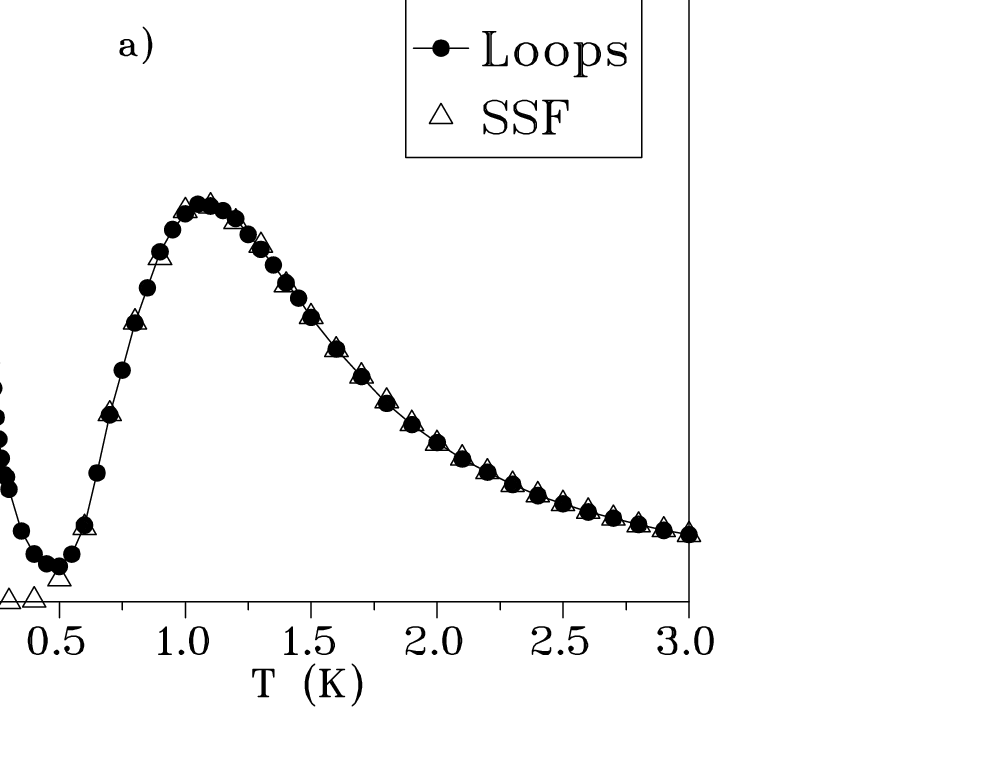
One can now return to the question asked earlier: “What happens to the numerically predicted phase transition to long-range order in real systems?” The numerical evidence for a first order transition to long-range order in the dipolar spin ice model is compelling [49, 50]. However, there has so far not been any reported experimental evidence for a phase transition in either Dy₂Ti₂O₇ [57] or Ho₂Ti₂O₇ [6, 9] down to approximately 60 mK. A possible, if not likely, reason for this failure of real spin ice materials to develop long range order at low temperature is that the spins in real materials are frozen and cannot thermally equilibrate since real systems “do not benefit” from the non-local type of spin dynamics such as the one employed in loop Monte Carlo simulations. Another possibility [33] is that perturbative $J_{ij}$ exchange interactions beyond nearest-neighbor in Eq. (8) frustrates the development of the long range order discussed above, pushing $T_{c}$ below the lowest temperature considered so far in experiments [57].

Before we briefly discuss in the last section of this chapter some avenues of research currently pursued in experimental studies of spin ices and related materials, we revisit the question of the microscopic origin of the ice rules in the dipolar spin ice model.

The Monte Carlo simulation results of Section 0.4.1 show that the spin ice phenomenology is due to long-range dipolar interactions. The mean-field theory calculations of Section 0.4.2 provide a first clue as to the mechanism behind the formation of the ice rules. However, neither method really explains why the dipolar spin ice obeys the ice rules. A succesful approach to answer this question was reported in Ref. [55].

The first important ingredient [60] is to note that the “two-in/two-out” ice rules on the pyrochlore lattice,

$$\sum_{\Delta}\sigma_{\Delta}^{z_{1}}+\sigma_{\Delta}^{z_{2}}+\sigma_{\Delta}^{z_{3}}+\sigma_{\Delta}^{z_{4}}=0\;,$$

(24)

where the sum is carried over up and down tetrahedra, is equivalent to a divergence-ree “spin field” $\vec{B}$, $\nabla\cdot{\vec{B}}=0$. These “lattice flux” are link variables that “live” on the diamond lattice dual to the pyrochlore lattice and $\nabla\cdot$ is the lattice divergence. By introducing a weight $\rho[{\vec{B}({\vec{r}})}]$ for nonzero flux (locally broken ice rules) of the form

$$\rho[{\vec{B}({\vec{r}})}]\propto\exp\left(-\frac{K}{2}\int[\vec{B}({\vec{r}})]^{2}d^{3}x\right)\;,$$

(25)

one can solve for the correlations

$\displaystyle\langle B_{u}(0)\cdot B_{v}(\vec{x})\rangle$

$\displaystyle\sim$

$\displaystyle\frac{3x_{u}x_{v}-r^{2}\delta_{uv}}{r^{5}}$

(26)

where $u,v$ are cartesian components. Equation (26) reveals that the local constraint, the ice rules, lead to spin-spin correlations that are dipolar-like at large distance.

The second important observation [55] it that one can construct a spin-ice-like toy model whose eigenmodes $\phi_{\vec{q}}^{\alpha}$ can be used to form a projector onto the ice-rule obeying ground states. Because of the asymptotic dipolar-like correlations that ice-rules obeying ground state possesses, according to Eq. (26), the real space matrix elements of this projector turns out to be the same as the dipolar part of the interactions (the second term) in $H_{\rm DSM}$ plus a small rapidly ($1/{r_{ij}}^{5}$) converging correction term, $V_{ab}(r_{ij})$. In other words, the dipolar interactions between the real magnetic moments is, up to a small rapidly decaying short-range corrections, a projector onto all possible ice-rule ground states. Hence, as a dipolar $\langle 111\rangle$ Ising system is cooled down below a temperature of the order of $D$, the spin configurations get energetically forced onto an ice-rule state, almost indiscriminently initially, when $V_{ab}(r_{ij})<T<D$. However, ultimately, the temperature reaches the scale of $V_{ab}(r_{ij})$ and a transition to a long-range ordered spin ice state, the one discussed in Section 0.4.3, occurs, provided ergodicity can be maintained [49, 50].

A possibly much simpler explanation has recently been proposed [61]. “Exploding” each point dipole into its constitutive magnetic (monopole) charges, and imposing that each tetrahedron unit cell is neutral (magnetic charge wise), automatically leads to the conclusion that all ice-rule obeying states are, again up to a small rapidly decaying short-range correction, a ground state of the microscopic magnetostatic dipolar interactions of Eq. (8) [61]. Those magnetic charges interact as $1/r$ for large inter-charge separation $r$. Magnetic field driven [61] and temperature driven [62] nucleation of those objects has been invoked to explain thermodynamic [61] and dynamical [62] properties of spin ice materials. We discuss below their possible experimental manifestation.

Because of the large magnetic moment of Dy³⁺ and Ho³⁺ in spin ice materials, even moderately small magnetic field can induce dramatic effects. Of particular interest is the “pinning” of the spins by a sufficently strong field on one [61, 63, 64, 65], two [32], three [32, 66] or the four [67] sites of a primitive tetrahedron cell, depending of the field orientation. This gives rise to interesting collective behaviors such as phase transitions to long range order [32, 66], topological Kasteleyn transitions [63, 65, 67], magnetization plateau states [61, 63] and a sort of magnetic monopole gas-liquid transition [61]. We briefly discuss some of the salient features characterizing the behavior of the system according to the direction of the magnetic field, $\vec{B}$.

References

- (1) G. H. Wannier, Phys. Rev. 79, 357 (1950); erratum Phys. Rev. B 7, 5017 (1973)
- (2) W. F. Giauque, M. F. Ashley, Phys. Rev. 43, 81 (1933)
- (3) W. F. Giauque, J. W. Stout, J. Am. Chem. Soc. 58, 1144 (1936)
- (4) L. Pauling, J. Am. Chem. Soc. 57, 2680 (1935)
- (5) M. J. Harris, S. T. Bramwell, D. F. McMorrow, T. Zeiske, K. W. Godfrey, Phys. Rev. Lett. 79, 2554 (1997)
- (6) M. J. Harris, S. T. Bramwell, T. Zeiske, D. F. McMorrow, P. J. C. King, J. Magn. Magn. Mater. 177, 757 (1998)
- (7) A. P. Ramirez, A. Hayashi, R. J. Cava, R. Siddharthan, Nature 399, 333 (1999)
- (8) S. T. Bramwell, M. J. P. Gingras, Science 294, 1495 (2001)
- (9) S. T. Bramwell, M. J. P. Gingras, P. C. W. Holdsworth, in: Frustrated Spin Systems, ed. by H. T. Diep (World Scientific Publishing, Singapore, 2004). p. 367
- (10) J. D. Bernal, R. H. Fowler, J. Chem. Phys. 1, 515 (1933)
- (11) J. M. Ziman, Models of Disorder:The Theoretical Physics of Homogeneously Disordered Systems, (Cambridge University Press, Cambridge, 1976)
- (12) J. F. Nagle, J. Math. Phys. 7, 1484 (1966)
- (13) P. W. Anderson, Phys. Rev. 102, 1008 (1956)
- (14) J. Villain, Z. Phys. B 33, 31 (1979)
- (15) J. N. Reimers, Phys. Rev. B 45, 7287 (1992)
- (16) R. Moessner, J. T. Chalker, Phys. Rev. B 58, 12049 (1998)
- (17) J. E. Greedan, J. of Materials Chemistry 11, 37 (2001)
- (18) J. S. Gardner, M. J. P. Gingras and J. E. Greedan, to appear in Rev. Mod. Phys. (2009)
- (19) J. S. Gardner, S. R. Dunsiger, B. D.Gaulin, M. J. P. Gingras, J. E. Greedan, R. F. Kiefl, M. D. Lumsden, W. A. MacFarlane, N. P. Raju, J. E. Sonier, I. Swainson, Z. Tun, Phys. Rev. Lett. 82, 1012 (1999)
- (20) J. E. Greedan, M. Sato, Y. Xu, F. S. Razavi, Solid State Commun. 59, 895 (1986)
- (21) B. D. Gaulin, J. N. Reimers, T. E. Mason, J. E. Greedan, Z. Tun, Phys. Rev. Lett. 69, 3244 (1992)
- (22) Y. Taguchi, Y. Oohara, H. Yoshizawa, N. Nagaosa, Y. Tokura, Science 291, 2573 (2001)
- (23) H. R. Molavian, M. J. P. Gingras, B. Canals, Phys. Rev. Lett. 98, 157204 (2007)
- (24) S. Rosenkranz, A. P. Ramirez, A. Hayashi, R. J. Cava, R. Siddharthan, B. S. Shastry, J. Appl. Phys. 84, 5914 (2000)
- (25) M. J. P. Gingras, B. C. den Hertog, M. Faucher, J. S. Gardner, S. R. Dunsiger, L. J. Chang, B. D. Gaulin, N. P. Raju, J. E. Greedan, Phys. Rev. B 62, 6496 (2000)
- (26) I. Mirebeau, P. Bonville, M. Hennion Phys. Rev. B 76, 184436 (2007)
- (27) A. Abragam, B. Bleaney, Electron Paramagnetic Resonance of Transition Ions, (Dover, 1986)
- (28) I. D. Ryabov, J. Magn. Reson. 140, 141 (1999)
- (29) C. Rudowicz, C. Y. Chung, J. Phys.: Condens. Matter 16, 1 (2004)
- (30) B. C. den Hertog, M. J. P. Gingras, Phys. Rev. Lett. 84, 3430 (2000)
- (31) S. T. Bramwell, M. J. Harris, B. C. den Hertog, M. J. P. Gingras, J. S. Gardner, D. F. McMorrow, A. R. Wildes, A. L. Cornelius, J. D. M. Champion, R. G. Melko, T. Fennell, Phys. Rev. Lett. 87, 047205 (2001)
- (32) J. P. C. Ruff, R. G. Melko, M. J. P. Gingras, Phys. Rev. Lett. 95, 097202 (2005)
- (33) T. Yavors’kii, T. Fennell, M. J. P. Gingras, S. T. Bramwell, Phys. Rev. Lett. 101, 037204 (2008)
- (34) S. H. Curnoe, Phys. Rev. B 78, 094418 (2008)
- (35) P. A. McClary, S. H. Curnoe, M. J. P. Gingras, J. Phys.: Conf. Ser. 145, 012032 (2009)
- (36) As a realistic figure of comparison between the spin-spin interactions and , the coupling constants and should be multiplied by the relevant products of matrix elements. Taking as a rough estimate for such products the magnitude squared of , for both Dy3+ with J=15/2 and Ho3+ with J=8, we still have and
- (37) R. Siddharthan, B. S. Shastry, A. P. Ramirez, A. Hayashi, R. J. Cava and S. Rosenkranz, Phys. Rev. Lett. 83, 1854 (1999)
- (38) However, in Ref. [33], was estimated using the crystal field ground state doublet wave functions. This gives a moment slightly less than 10
- (39) I. Mirebeau, A. Apetrei, J. Rodríguez-Carvajal, P. Bonville, A. Forget, D. Colson, V. Glazkov, J. P. Sanchez, O. Isnard, E. Suard, Phys. Rev. Lett. 94, 246402 (2005)
- (40) T. Fennell, O. A. Petrenko, B. Fåk, J. S. Gardner, S. T. Bramwell, B. Ouladdiaf, Phys. Rev. B 72, 224411 (2005)
- (41) K. Binder, A. P. Young, Rev. Mod. Phys. 58, 801 (1986)
- (42) S. T. Bramwell and M. J. Harris, J. Phys.: Condens. Matter 10, L215 ((1998)
- (43) In Refs. [30, 31], a quantity and between the Ising variables was employed. The reason for introducing these two rescaled couplings becomes clear when considering Eq. (14)
- (44) X. Ke, R. S. Freitas, B. G. Ueland, G. C. Lau, M. L. Dahlberg, R. J. Cava, R. Moessner, P. Schiffer, Phys. Rev. Lett. 99, 137203 (2007)
- (45) B. C. den Hertog, M. J. P. Gingras, S. T. Bramwell, M. J. Harris, arXiv:cond-mat/9912220 (1999)
- (46) A. L. Cornelius, J. S. Gardner, Phys. Rev. B, 64, 060406 (2001)
- (47) H. Kadowaki, Y. Ishii, K. Matsuhira, Y. Hinatsu, Phys. Rev. B 65, 144421 (2002)
- (48) X. Ke, B. G. Ueland, D. V. West, M. L. Dahlberg, R. J. Cava, P. Schiffer, Phys. Rev. B 76, 214413 (2007)
- (49) R. G. Melko, B. C. den Hertog, M. J. P. Gingras, Phys. Rev. Lett. 87, 067203 (2001)
- (50) R. G. Melko, M. J. P. Gingras, J. Phys.: Condensed Matter 16, R1277 (2004)
- (51) C. Kittel, Introduction to Solid State Physics, 8th edn. (Wiley, 2005), Appendix B
- (52) M. J. P. Gingras, B. C. den Hertog, Can. J. Phys. 79, 1339 (2001)
- (53) J. N. Reimers, A. J. Berlinsky, A. C. Shi, Phys. Rev. B 43, 865 (1991)
- (54) M. Enjalran, M J. P. Gingras, Phys. Rev. B 70, 174426 (2004)
- (55) S. V. Isakov, R. Moessner, S. L. Sondhi, Phys. Rev. Lett. 95, 217201 (2005)
- (56) M. Enjalran, M J. P. Gingras, arXiv:cond-mat/0307151v1 (2003)
- (57) H. Fukazawa, R. G. Melko, R. Higashinaka, Y. Maeno, M. J. P. Gingras, Phys. Rev. B 65, 054410 (2002)
- (58) G. T. Barkema, M. E. J. Newman, Phys. Rev. E 57, 1155 (1998)
- (59) M. E. J. Newmann and G. T. Barkema, Monte Carlo Methods in Statistical Physics, (Clarendon Press, Oxford, 1999)
- (60) S. V. Isakov, K. Gregor, R. Moessner, S. L. Sondhi Phys. Rev. Lett. 93, 167204 (2004)
- (61) C. Castelnovo, R. Moessner, S. L. Sondhi, Nature 451, 42 (2008)
- (62) L. D. C. Jaubert, P. C. W. Holdsworth, arXiv:0903.1074 (2009). To appear in Nature Physics (2009).
- (63) R. Moessner, S. L. Sondhi, Phys. Rev. B 68, 064411 (2003)
- (64) Y. Tabata, H. Kadowaki, K. Matsuhira, Z. Hiroi, N. Aso, E. Ressouche, Fåk, Phys. Rev. Lett. 97, 257205 (2006)
- (65) T. Fennell, S. T. Bramwell, D. F. McMorrow, P. Manuel P, A. R. Wildes, Nature Physics 8, 566 (2007)
- (66) R. Higashinaka, Y. Maeno Phys. Rev. Lett. 95, 237208 (2005)
- (67) L. Jaubert, J. T. Chalker, P. C. W. Holdsworth, R. Moessner, Phys. Rev. Lett. 100, 067207 (2008)
- (68) Z. Hiroi, K. Matsuhira, M Ogata, J. Phys. Soc. Jpn. 72, 3045 (2003)
- (69) S.-i. Yoshida, K. Nemoto, K. Koh Wada, J. Phys. Soc. Jpn. 73, 1619 (2004)
- (70) J. P. Clancy, J. P. C. Ruff, S. R. Dunsiger, Y. Zhao, H. A. Dabkowska, J. S. Gardner, Y. Qiu, J. R. D. Copley, T. Jenkins, B. D. Gaulin, Phys. Rev. B 79, 014408 (2009)
- (71) T. Sakakibara, T. Tayama, Z. Hiroi, K. Matsuhira, S. Takagi, Phys. Rev. Lett. 90, 207205 (2003)
- (72) H. Aoki, T. Sakakibara, K. Matsuhira, Z. Hiroi, J. Phys. Soc. Jpn. 73, 2851 (2004)
- (73) M. J. Harris, S. T. Bramwell, P. C. W. Holdsworth, J. D. Champion, Phys. Rev. Lett. 81, 4496 (1998)
- (74) J. Snyder, B. G. Ueland, J. S. Slusky, H. Karunadasa, R. J. Cava, A. Mizel, P. Schiffer, Phys. Rev. Lett. 91, 107201 (2003)
- (75) J. Snyder, B. G. Ueland, J. S. Slusky, H. Karunadasa, R. J. Cava, P. Schiffer, Phys. Rev. B 69, 064414 (2004)
- (76) G. Ehlers, J. S. Gardner, C. H. Booth, M. Daniel, K. C. Kam, A. K. Cheetham, D. Antonio, H. E. Brooks, A. L. Cornelius, S. T. Bramwell, J. Lago, W. Häussler, N. Rosov Phys. Rev. B 73, 174429 (2006)
- (77) J. P. Sutter, S. Tsutsui, R. Higashinaka, Y. Maeno, O. Leupold, A. Q. Baron, Phys. Rev. B 75, 140402 (2007)
- (78) J. Lago J, S. J. Blundell, C. Baines, J. Phys.: Condensed Matter 19, 326210 (2007)
- (79) G. Ehlers, E. Mamontov, M. Zamponi, K. C. Kam, J. S. Gardner, Phys. Rev. Lett. 102, 016405 (2009)
- (80) S. Nakatsuji, Y. Machida, Y. Maeno, T. Tayama, T. Sakakibara, J. van Duijn, L. Balicas, J. N. Millican, R. T. Macaluso, J. Y. Chan, Phys. Rev. Lett. 96, 087204 (2006)
- (81) Y. Machida, S. Nakatsuji, Y. Maeno, T. Tayama, T. Sakakibara, S. Onoda, Phys. Rev. Lett. 98, 057203 (2007)
- (82) A. Ikeda, H. Kawamura, J. Phys. Soc. Jpn. 77, 073707 (2008)
- (83) R. F. Wang, C. Nisoli, R. S. Freitas, J. Li, W. McConville, B. J. Cooley, M. S. Lund, N. Samarth, C. Leighton, V. H. Crespi, P. Schiffer, Nature 439, 303 (2006)
- (84) C. Nisoli, R. F. Wang, J. Li, W. F. McConville, P. E. Lammert, P. Schiffer, V. H. Crespi, Phys. Rev. Lett. 98, 217203 (2007)
- (85) A. Libál, C. Reichhardt, C. J. Reichhardt Phys. Rev. Lett. 97, 228302 (2006)
- (86) G. C. Lau, R. S. Freitas, B. G. Ueland, B. D. Muegge, E. L. Duncan, P. Schiffer, R. J. Cava, Nature Physics 2, 249 (2006)
- (87) G. C. Lau, B. D. Muegge, T. M. McQueen, E. L. Duncan, R. J. Cava, J. Sol. State Chemistry 179, 3136 (2006)
- (88) G. C. Lau, R. S. Freitas, B. G. Ueland, M. L. Dahlberg, Q. Huang, H. W. Zandbergen, P. Schiffer, R. J. Cava, Phys. Rev. B 76, 054430 (2007)
- (89) P. Dalmas de Réotier, A. Yaouanc, L. Keller, A. Cervellino, B. Roessli, C. Baines, A. Forget, C. Vaju, P. C. Gubbens, A. Amato, P. J. King Phys. Rev. Lett. 96, 127202 (2006)
- (90) F. Bert, P. Mendels, A. Olariu, N. Blanchard, G. Collin, A. Amato, C. Baines, A. D. Hillier, Phys. Rev. Lett. 97, 117203 (2006)
- (91) S. R. Giblin, J. D. Champion, H. D. Zhou, C. R. Wiebe, J. S. Gardner, I. Terry, S. Calder, T. Fennell, S. T. Bramwell, Phys. Rev. Lett. 101, 237201 (2008)
- (92) H. D. Zhou, C. R. Wiebe, J. A. Janik, L. Balicas, Y. J. Yo, Y. Qiu, J. R. Copley, J. S. Gardner, Phys. Rev. Lett. 101, 227204 (2008)