Performance Assessment of MIMO-BICM
Demodulators based on System Capacity
Abstract
We provide a comprehensive performance comparison of soft-output and hard-output demodulators in the context of non-iterative multiple-input multiple-output bit-interleaved coded modulation (MIMO-BICM). Coded bit error rate (BER), widely used in literature for demodulator comparison, has the drawback of depending strongly on the error correcting code being used. This motivates us to propose a code-independent performance measure in terms of system capacity, i.e., mutual information of the equivalent modulation channel that comprises modulator, wireless channel, and demodulator. We present extensive numerical results for ergodic and quasi-static fading channels under perfect and imperfect channel state information. These results reveal that the performance ranking of MIMO demodulators is rate-dependent. Furthermore, they provide new insights regarding MIMO-BICM system design, i.e., the choice of antenna configuration, symbol constellation, and demodulator for a given target rate.
Index Terms:
MIMO, BICM, performance limits, soft demodulation, system capacity, log-likelihood ratioEDICS Category: MSP-CAPC, MSP-CODR
I Introduction
I-A Background
Bit-interleaved coded modulation (BICM) [2, 3] has been conceived as a pragmatic approach to coded modulation. It has received a lot of attention in wireless communications due to its bandwidth and power efficiency and its robustness against fading. For single-antenna systems, BICM with Gray labeling can approach channel capacity [2, 4]. These advantages have motivated extensions of BICM to multiple-input multiple-output (MIMO) systems [5, 6, 7].
In MIMO-BICM systems, the optimum demodulator is the soft-output maximum a posteriori (MAP) demodulator, which provides the channel decoder with log-likelihood ratios (LLRs) for the code bits. Due to its high computational complexity, numerous alternative demodulators have been proposed in the literature. Applying the max-log approximation [7] to the MAP demodulator reduces complexity without significant performance loss and leads to a search for data vectors minimizing a Euclidean norm. Exact implementations of the max-log MAP detector based on sphere decoding have been presented in [8, 9, 10]; sphere decoder variants in which the Euclidean norm is replaced with the norm have been proposed in [11, 12]. However, the complexity of sphere decoding grows exponentially with the number of transmit antennas [9]. An alternative demodulator that yields approximations to the true LLRs is based on semidefinite relaxation (SDR) and has polynomial worst-case complexity [13, 14].
Several demodulation schemes use a list of candidate data vectors to obtain approximate LLRs. The size of the candidate list offers a trade-off between performance and complexity. The candidate list can be generated using i) tree search techniques as with the list sphere decoder (LSD) [15], ii) lattice reduction (LR) techniques [16, 17, 18, 19, 20], or iii) bit flipping techniques, i.e., flipping some of the bits in the label of a data vector obtained by hard detection, e.g. [21].
MIMO demodulators with still smaller complexity consist of a linear equalizer followed by per-layer scalar soft demodulators. This approach has been studied using zero-forcing (ZF) equalization [22, 23] and minimum mean-square error (MMSE) equalization [24, 25]. The soft interference canceler (SoftIC) proposed in [26] iteratively performs parallel MIMO interference cancelation by subtracting an interference estimate which is computed using soft symbols from the preceding iteration.
Hard-output MIMO demodulators are alternatives to soft demodulators that provide tentative decisions for the code bits but no associated reliability information. Among the best-known schemes here are maximum likelihood (ML), ZF, and MMSE demodulation [27] and successive interference cancelation (SIC) [28, 29, 30].
I-B Contributions
In the context of MIMO-BICM, the performance of the MIMO demodulators listed above has mostly been assessed in terms of coded bit error rate (BER) using a specific channel code. These BER results depend strongly on the channel code and hence render an impartial demodulator comparison difficult.
In this paper, we advocate an information theoretic approach for assessing the performance of (soft and hard) MIMO demodulators in the context of non-iterative11 1 A performance assessment of soft-in soft-out demodulators in iterative BICM receivers requires a completely different approach and is thus beyond the scope of this paper. (single-shot) BICM receivers (see also [1]). Inspired by [5], we propose the mutual information between the modulator input bits and the associated MIMO demodulator output as a code-independent performance measure. This quantity can be interpreted as system capacity (maximum rate allowing for error-free information recovery) of an equivalent “modulation” channel that comprises modulator and demodulator in addition to the physical channel. This approach establishes a systematic framework for the assessment of MIMO demodulators. We note that ZF-based and max-log demodulation have been compared in a similar spirit in [23].
Using Monte Carlo simulations, this paper provides extensive performance evaluations and comparisons for the above-mentioned MIMO demodulators in terms of system capacity, considering different system configurations in fast and quasi-static fading. We also investigate the performance loss of the various demodulation schemes under imperfect channel state information (CSI). Due to lack of space, only a part of our numerical results is shown here. Further results for other antenna configurations, symbol constellations, and bit mappings can be found in a supporting document [31].
Our results allow for several conclusions. Most importantly, we found that no universal performance ranking of MIMO demodulators exists, i.e., the ranking depends on the information rate or, equivalently, on the signal-to-noise ratio (SNR). As an example, soft MMSE outperforms hard ML at low rates while at high rates it is the other way around. We also verify this surprising observation in terms of BER simulations using low-density parity-check (LDPC) codes. Finally, we use our numerical results to develop practical guidelines for the design of MIMO-BICM systems, i.e., which antenna configuration, symbol constellation, and demodulator to choose in order to achieve a certain rate with minimum SNR.
I-C Paper Organization
The rest of this paper is organized as follows. Section II discusses the MIMO-BICM system model and Section III proposes system capacity as performance measure. In Sections IV and V, we assess the system capacity achievable with the MIMO-BICM demodulators referred to above for the case of fast fading. Section VI analyzes the impact of imperfect channel state information (CSI) on the demodulator performance, and Section VII investigates the rate-versus-outage tradeoff of selected demodulators in quasi-static environments. In Section VIII, we summarize key observations and infer practical system design guidelines. Finally, conclusions are provided in Section IX.
II System Model
II-A MIMO-BICM Transmission Model
A block diagram of our MIMO-BICM model is shown in Fig. 1. The information bits are encoded using an error-correcting code and is then passed through a bitwise interleaver . The interleaved code bits are demultiplexed into antenna streams (“layers”). In each layer , groups of code bits , , ( denotes symbol time) are mapped via a one-to-one function to (complex) data symbols from a symbol alphabet of size . Specifically, , where is referred to as the bit label of . The transmit vector is given by22 2 The superscripts and denote transposition and Hermitian transposition, respectively. Furthermore, is the -fold Cartesian product of , denotes expectation, and is the (Euclidean) norm. and satisfies the power constraint . It carries interleaved code bits , , with . We will for simplicity write and as shorthand for the mapping and its inverse.
Assuming flat fading, the receive vector ( denotes the number of receive antennas) is given by
| (1) |
where is the channel matrix, and is a noise vector with independent identically distributed (i.i.d.) circularly symmetric complex Gaussian elements with zero mean and variance . In most of what follows, we will omit the time index for convenience.
At the receiver, the optimum demodulator uses the received vector and the channel matrix to calculate LLRs for all code bits , , carried by . In practice, the use of suboptimal demodulators or of a channel estimate will result in approximate LLRs . The LLRs are passed through the deinterleaver and then on to the channel decoder that delivers the detected bits .
II-B Optimum Soft MAP Demodulation
Assuming i.i.d. uniform code bits (as guaranteed, e.g., by an ideal interleaver), the optimum soft MAP demodulator calculates the exact LLR for based on according to [7]
| (2) |
Here, is the probability mass function (pmf) of the code bits conditioned on and , and denote the complementary sets of transmit vectors for which and , respectively (note that ). Unfortunately, computation of (2) has complexity , i.e., exponential in the number of transmit antennas. For this reason, several suboptimal demodulators have been proposed which promise near-optimal performance while requiring a lower computational complexity. The aim of this work is to provide a fair performance comparison of these demodulators.
III System Capacity
In order for the information rates discussed below to have interpretations as ergodic capacities, we consider a fast fading scenario where the channel is a stationary, finite-memory process. We recall that the ergodic capacity with Gaussian inputs is given by[32]
| (3) |
(here, denotes the identity matrix). The non-ergodic regime (slow fading) is discussed in Section III-D.
III-A Capacity of MIMO Coded Modulation
In a coded modulation (CM) system with equally likely transmit vectors and no CSI at the transmitter, the average mutual information in bits per channel use (bpcu) is given by (cf. [5])
| (4) |
Here, we used the conditional probability density function (pdf) (cf. (1))
| (5) |
In the following, we will refer to as CM capacity [2] (sometimes, is alternatively termed constellation-constrained capacity). It is seen from (4) that ; in fact, the last term in (4) may be interpreted as a penalty term resulting from the noise and MIMO interference.
Using the fact that the mapping between the symbol vector and the associated bit label is one-to-one and applying the chain rule for mutual information [33, page ] to (4) leads to
| (6) | ||||
here, denotes the entropy function. The single-antenna equivalent of (6) served as a motivation for multilevel coding and multistage decoding, which can indeed achieve CM capacity [4]. Multilevel coding for multiple antenna systems has been considered in [34].
III-B Capacity of MIMO-BICM
In the following, we assume an ideal, infinite-length bit interleaver33 3 In practice, this means that the interleaver needs to be much longer than the codewords transmitted over the channel. which allows us to treat the BICM system as a set of independent parallel memoryless binary-input channels as in [2, Section III.A]. Using the assumption of i.i.d. uniform code bits, the maximum rate achievable with BICM is given by (cf. [5])
| (7) | ||||
where44 4 By and we respectively denote the th element of the vector and the element in row and column of the matrix . denotes the th bit in the label of . Since conditioning reduces entropy [33, page ], a comparison of (6) and (7) reveals that [34]
The gap increases with and and depends strongly on the symbol labeling [7]. For single-antenna BICM systems with Gray labeling, this gap has been shown to be negligible [2, 4]; however, for MIMO systems (see Section IV) and at low SNRs in the wideband regime [3] it can be significant. The capacity loss can be attributed to the fact that the BICM receiver neglects the dependencies between the transmitted code bits. Under the unrealistic assumption of perfectly known channel SNR, multilevel coding with multistage decoding can in principle avoid such a capacity loss but suffers from error propagation [4, 34]. BICM does not require the channel SNR at the transmitter and can be considered more robust. A hybrid version of CM and BICM whose complexity and performance is between the two was presented in [34]. Furthermore, augmenting BICM with space-time mappings can be beneficial (cf. [35, 34]) but is not considered here due to space limitations.
It can be shown that the log-likelihood ratio in (2) is a sufficient statistic [36] for given and . Therefore, (7) can be rewritten as
| (8) |
Hence, can be interpreted as the capacity of an equivalent channel with inputs and outputs (cf. Fig. 1). This channel is characterized by the conditional pdf , which usually is hard to obtain analytically, however.
III-C System Capacity and Demodulator Performance
Motivated by the interpretation of as the system capacity of BICM using the optimum MAP demodulator, we propose to measure the performance of sub-optimal MIMO-BICM demodulators via the system capacity of the associated equivalent “modulation” channel with binary inputs and the approximate LLRs as continuous outputs (cf. Fig. 1). This channel is described by the conditional pdf . Its system capacity is defined as the mutual information between and , which can be shown to equal
| (9) |
where . We emphasize that the system capacity provides a performance measure for MIMO (soft) demodulators that is independent of the outer channel code. In fact, it has an intuitive operational interpretation as the highest rate achievable (in the sense of asymptotically vanishing error probability) in a BICM system with independent parallel channels (assumption of an ideal infinite-length interleaver, cf. [2, Section III.A]), using the specific demodulator which produces . Since is derived from and , the data processing inequality [33, page ] implies that with equality if is a one-to-one function of . The performance of a soft demodulator can thus be measured in terms of the gap . Of course, the information theoretic performance measure in (9) does not take into account complexity issues and it has to be expected that a reduction of the gap in general can only be achieved at the expense of increasing computational complexity.
We caution the reader that the rates in (8) and (9) are sums of mutual informations for the individual code bits carried by one symbol vector. Indeed, the pdfs and in general depend on the code bit position , even though for certain systems (e.g. 4-QAM modulation) the code bit protection and LLR statistics are independent of the bit position for reasons of symmetry. Achieving (8) and (9) thus requires channel encoders and decoders that take the bit position into account. When the channel code fails to use this information, the rate loss is small provided that the mapping protects different code bits roughly equally against noise and interference.
III-D Non-Ergodic Channels
In the case of quasi-static or slow fading [37], the channel is random but constant over time, i.e., each codeword can extend over only one channel realization. Here, the ergodic capacity of the modulation channel is no longer operationally meaningful [37, 38]. Instead we consider the outage probability
| (10) |
where is a random variable defined as
Here, denotes the conditional mutual information, which is evaluated with in place of (cf. (9)). Note that the ergodic system capacity in (9) equals . The outage probability can be interpreted as the smallest codeword error probability achievable at rate [38]. A closely related concept is the -capacity of the equivalent modulation channel, defined as
| (11) |
The -capacity may be interpreted as the maximum rate for which a codeword error probability less than can be achieved. Rates smaller than are referred to as -achievable rates [38]. If is a continuous and increasing function of (which is usually the case in practice), it holds that .
III-E Generalized Mutual Information
The operational interpretation of our performance measure as the largest achievable rate for a BICM system using a given demodulator requires the assumption of an ideal infinite-length interleaver. With a finite-length interleaver, the parallel channels (i.e., the different bits in a given symbol vector) are not independent in general; here, achievable rates can be characterized in terms of the generalized mutual information (GMI) which is obtained by treating the BICM receiver as a mismatched decoder [39, 3, 40]. For the case of optimum soft MAP demodulation (cf. (2)), the BICM capacity using the independent parallel-channel model coincides with the GMI [40]. We recently provided a non-straightforward extension of this result by showing that the GMI of a BICM system with suboptimal demodulators augmented with scalar LLR correction (see Section IV-D) coincides with the system capacity in (9) obtained for the parallel-channel model [41].55 5 We note that the LLR correction leaves the mutual information which underlies system capacity unchanged. Scalar LLR correction has been used previously to provide the binary decoder with accurate reliability information [36, 42, 43, 44, 45]. The GMI of a BICM system with finite interleaver and LLR-corrected suboptimal demodulators can thus efficiently be computed by evaluating (9) [41]; this provides additional justification for the use of (9) as a code-independent performance measure for approximate demodulators. We note that a GMI-based analysis of BICM with mismatched decoding metrics that generalizes our work in [41] has recently been presented in [46].
IV Baseline MIMO-BICM Demodulators
In this section, we first review max-log and hard ML demodulation as well as linear MIMO demodulators and then we provide results illustrating their performance in terms of system capacities. These demodulators serve as baseline systems for later demodulator performance comparisons in Section V. We note that max-log and hard ML MIMO demodulators have the highest complexity among all soft and hard demodulation schemes, respectively, whereas linear MIMO demodulators are most efficient computationally. Due to space limitations, we only state the complexity order of each demodulator in the following and we give references that provide more detailed complexity analyses.
IV-A Max-Log and Hard ML Demodulator
Applying the max-log approximation to (2) simplifies the LLR computation to a minimum distance problem and results in the approximate LLRs [7]
| (12) |
This expression can be implemented easier than (2) since it avoids the logarithm and exponential functions. However, computation of in (12) still requires two searches over sets of size . Sphere decoder implementations of (12) are presented in [8, 10].
Hard vector ML demodulation amounts to the minimum distance problem
| (13) |
This optimization problem can be solved by exhaustive search or using a sphere decoder; in both cases, the computational complexity scales exponentially with the number of transmit antennas. The detected code bits corresponding to (13) are obtained via the one-to-one mapping between code bits and symbol vectors, i.e., . It can be shown that the code bits obtained by the hard ML detector correspond to the sign of the corresponding max-log LLRs in (12), i.e., where denotes the unit step function. When it comes to computing the system capacity with hard-output demodulators, the only difference to soft-output demodulation is the discrete nature of the outputs of the equivalent “modulation” channel, which here becomes a binary channel. Consequently, the integral over in (9) is replaced with a summation over .
IV-B Linear Demodulators
In the following, is the LLR corresponding to (the th bit in the bit label of the th symbol ). Soft demodulators with extremely low complexity can be obtained by using a linear (ZF or MMSE) equalizer followed by per-layer max-log LLR calculation according to
| (14) |
Here, denotes the set of (scalar) symbols whose bit label at position equals , is an estimate of the symbol in layer provided by the equalizer, and is an equalizer-specific weight (see below). We emphasize that calculating LLRs separately for each layer results in a significant complexity reduction. In fact, calculating the symbol estimates using a ZF or MMSE equalizer requires operations; furthermore, the complexity of evaluating (14) for all code bits scales as , i.e., linearly in the number of antennas[24, 25].
Equalization-based hard bit decisions can be obtained by quantization of the equalizer output with respect to (denoted by ), followed by the demapping, i.e., . Again, the detected code bits correspond to the sign of the LLRs, i.e., .
IV-B1 ZF-based Demodulator [22, 23]
Here, the first stage consists of ZF equalization, i.e.,
| (15) |
where the post-equalization noise vector has correlation matrix
| (16) |
Subsequently, approximate bit LLRs are obtained according to (14) with symbol estimate and weight factor .
IV-B2 MMSE-based Demodulator [25, 24]
Here, the first stage is an MMSE equalizer that can be written as (cf. (15) and (16))
| (17) |
Approximate LLRs are then calculated according to (14) with
where . Here, denotes the output of the unbiased MMSE equalizer, which is preferable to a biased MMSE equalizer for non-constant modulus modulation schemes such as -QAM and -QAM [47]; in the remainder we will thus restrict to unbiased soft and hard MMSE demodulators.
IV-C Capacity Results
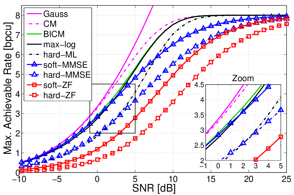
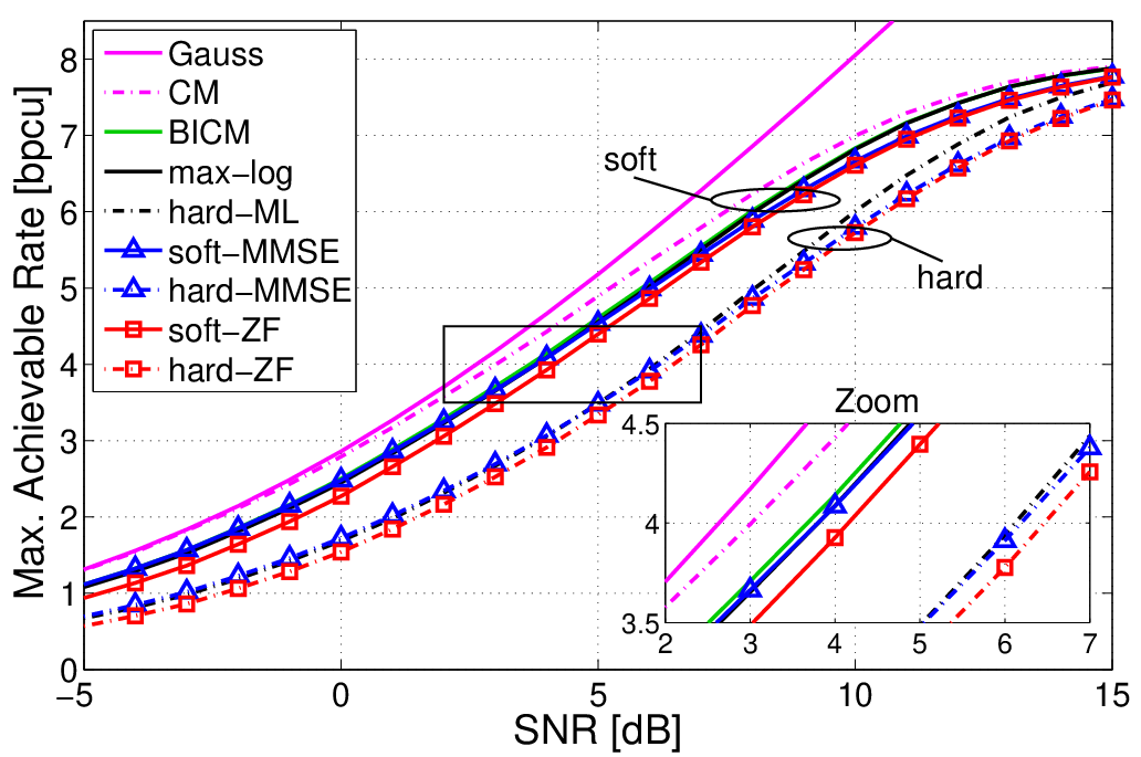
We next compare the performance of the above baseline demodulators (i.e., max-log, hard ML, MMSE and ZF) in terms of their maximum achievable rate (ergodic system capacity, see (9)). In addition, the CM capacity in (4), the MIMO-BICM capacity in (7) (corresponding to the system capacity of the optimum soft MAP demodulator in (2)), and the Gaussian input channel capacity in (3) are shown as benchmarks. Throughout the paper, all capacity results have been obtained for spatially i.i.d. Rayleigh fading, with all fading coefficients normalized to unit variance.
The pdfs required for evaluating (9) are generally hard to obtain in closed form. Thus, we measured these pdfs using Monte Carlo simulations and then evaluated all integrals numerically. Based on the results in [48], we numerically optimized the binning (used to measure the pdfs) in order to reduce the bias and variance of the mutual information estimates (see Appendix A for more details). The capacity results (obtained with fading realizations) are shown in Fig. 2 in bits per channel use versus SNR . In the following, in some of the plots we show insets that provide zooms of the capacity curves around a rate of bpcu.
Fig. 2(a) pertains to the case of MIMO with Gray-labeled -QAM (here, ). At a target rate of bpcu, the SNR required for CM and Gaussian capacity is virtually the same, whereas that for BICM is larger by about dB. The SNR penalty of using max-log demodulation instead of soft MAP is about dB. Furthermore, hard ML demodulation requires a dB higher SNR to achieve this rate than max-log demodulation; for soft and hard MMSE demodulation the SNR gaps to max-log are dB and dB, respectively, while for soft and hard ZF demodulation they respectively equal dB and dB. An interesting observation in this scenario is the fact that at low rates, soft and hard MMSE demodulation slightly outperform max-log and hard ML demodulation, respectively, whereas at high rates MMSE demodulation degrades to ZF performance. Hard MMSE demodulation can outperform hard ML demodulation since the latter minimizes the vector symbol error probability whereas our system capacity is defined on the bit level. Surprisingly, at low rates soft MMSE essentially coincides with BICM capacity. Moreover, soft MMSE demodulation outperforms hard ML demodulation at low-to-medium rates whereas at high rates it is the other way around (the cross-over can be seen at about bpcu). These observations reveal the somewhat unexpected fact that the demodulator performance ranking is not universal but depends on the target rate (or equivalently, the target SNR), even if the number of antennas, the symbol constellation, and the labeling are fixed. Similar observations apply to -QAM instead of -QAM and to set-partitioning labeling instead of Gray labeling (see [31]). Apart from a general shift of all curves to higher SNRs, the larger constellation and/or the different labeling strategy causes an increase of the gap between CM capacity and BICM capacity. The gaps between hard ML, hard MMSE, and soft ZF demodulation are significantly smaller, though, in this case (soft ZF outperforms hard MMSE for rates above bpcu and approaches hard ML for rates around bpcu). When decreasing the antenna configuration to a system, we observed that soft ZF outperforms hard ML demodulation for low-to-medium rates, e.g., by about dB at bpcu with -QAM [31].
The situation changes for the case of a MIMO system with Gray-labeled -QAM (again ), shown in Fig. 2(b). The increased SNR gap between CM and BICM capacity implied by the larger constellation is compensated by having more receive than transmit antennas (this agrees with observations in [7]). In addition, the performance differences between the individual demodulators are significantly reduced, revealing an essential distinction being between soft and hard demodulators. Having helps the linear demodulators approach their non-linear counterparts even at larger rates, i.e., soft ZF/MMSE perform close to max-log and hard ZF/MMSE perform close to hard ML, with an SNR gap of about dB between hard and soft demodulators. Note that in this scenario soft MMSE and soft ZF both outperform hard ML demodulation at all rates.
IV-D BER Performance
Even though we advocate a demodulator comparison in terms of system capacity, the cross-over of some of the capacity curves prompts a verification in terms of the BER of soft and hard MMSE demodulation as well as max-log and hard ML demodulation. We consider a MIMO-BICM system with Gray-labeled -QAM in conjunction with irregular LDPC codes66 6 The LDPC code design was performed using the web-tool at http://lthcwww.epfl.ch/research/ldpcopt. [49] of block length . For the case of soft demodulation, the LDPC codes were designed for an additive white Gaussian noise (AWGN) channel whereas for the case of hard demodulators the design was for a binary symmetric channel. At the receiver, message-passing LDPC decoding [49] was performed. In the case of hard demodulation, the message-passing decoder was provided with the LLRs
| (18) |
where , the cross-over probability of the equivalent binary channel, was determined via Monte Carlo simulations. With the soft demodulators, we performed an LLR correction via a lookup table as in [45]. Using LLR correction for soft demodulators and (18) for hard output demodulators is critical in order to provide the channel decoder with accurate reliability information [36, 42, 43, 44, 45, 41].
The BERs obtained for code rates of ( bpcu) and ( bpcu) are shown in Fig. 3(a) and (b), respectively. Vertical lines indicate the respective capacity limits, i.e., the minimum SNR required for the target rate according to Fig. 2(a). It is seen that the LDPC code designs are less than dB away from the capacity limits. At low rates soft MMSE performs best and hard ML performs worst whereas at high rates max-log and hard MMSE give the best and worst results, respectively. More specifically, at rate soft MMSE outperforms max-log and hard ML demodulation by dB and dB, respectively (cf. Fig. 3(a)); at rate soft MMSE performs dB poorer than hard ML and dB poorer than max-log (cf. Fig. 3(b)). These BER results confirm the capacity-based observation that there is no universal (i.e., rate- and SNR-independent) demodulator performance ranking. We note that the block error rate results in [50] imply similar conclusions, even though not explicitly mentioned in that paper.


V Other Demodulators
In the following, we study the system capacity of several other MIMO-BICM demodulators that differ in their underlying principle and their computational complexity. Unless stated otherwise, capacity results shown in this section pertain to a MIMO system with -QAM using Gray labeling (). The results for asymmetric MIMO systems with -QAM (shown in [31] but not here) essentially confirm the general distinction between hard and soft demodulators observed in connection with Fig. 2(b).
V-A List-based Demodulators
In order to save computational complexity, (12) can be approximated by decreasing the size of the search set, i.e., replacing with a smaller set. Usually, this is achieved by generating a (non-empty) candidate list and restricting the search in (12) to this list, i.e.,
| (19) |
As the number of operations required to compute the metric for each candidate of the list is , the overall computational complexity of the metric evaluations and minima searches in (19) scales as . Thus, the list size allows to trade off performance for complexity savings. A larger list size generally incurs higher complexity but yields more accurate approximations of the max-log LLRs. For a fixed list size, the performance further depends on how the list is generated. In the following, we consider two types of list generation, one based on sphere decoding and the other on bit flipping.
V-A1 List Sphere Decoder (LSD)
The LSD proposed in [15] uses a simple modification of the hard-decision sphere decoder [51] to generate the candidate list such that it contains the symbol vectors with the smallest ML metric (thus, by definition contains the hard ML solution in (13)). If the th bit in the labels of all equals , the set is empty and (19) cannot be evaluated. Since in this case there is strong evidence for (at least if is not too small), the LLR is set to a prescribed positive value . Analogously, in case is empty.
While the LSD may offer significant complexity savings compared to max-log demodulation, statements about its computational complexity are difficult and depend strongly on the actual implementation of the sphere decoder as well as the choice of the list size (for details we refer to [15]). We note that the case implies ; thus, such that (19) equals the max-log demodulator in (12). The other extreme is a list size of one, i.e., (cf. (13)), in which case either or is empty (depending on the bit label of ); here, where and thus the LSD output is equivalent to hard ML demodulation (except for the choice of , which is irrelevant, however, for capacity).
Capacity Results. Fig. 4 shows the maximum rates achievable with an LSD for various list sizes. BICM and soft MMSE capacity are shown for comparison. Note that with -QAM and , and correspond to max-log and hard ML demodulation, respectively. It is seen that with increasing list size the gap between LSD and max-log decreases rapidly, specifically at high rates. In particular, the LSD with list sizes of is already quite close to max-log performance. However, at low rates LSD (even with large list sizes) is outperformed by soft MMSE: below dB, dB, and dB the system capacity of soft MMSE is higher than that of LSD with list size , , and , respectively. Similar observations apply to other antenna configurations and symbol constellations (see [31]).

V-A2 Bit Flipping Demodulators
Another way of generating the candidate list , proposed in [21], is to flip some of the bits in the label of the hard ML symbol vector estimate in (13). More generally, the ML solution can be replaced by a symbol vector obtained with an arbitrary hard-output demodulator (e.g., hard ZF and MMSE demodulation). Let denote the bit label of . The candidate list then consists of all symbol vectors whose bit label has Hamming distance at most from , i.e., . Here, denotes the Hamming distance between two bit labels and . This list can be generated by systematically flipping up to bits in and mapping the results to symbol vectors. The resulting list size is given by . Here, the structure of the list generated with bit flipping allows to reduce the complexity per candidate to ,77 7 Changing the value of a particular bit changes only one symbol in the symbol vector. Thus, the residual in (19) can be easily updated by adding an appropriately scaled column of . This requires only instead of operations. giving an overall complexity of (plus the operations required for the initial estimate). For , and (19) reduces to max-log demodulation; furthermore, with and there is and (19) becomes equivalent to hard ML demodulation. In contrast to the LSD, bit flipping with ensures that and are nonempty so that (19) can always be evaluated.
Capacity Results. Fig. 5 shows the maximum rates achievable with bit flipping demodulation where the initial symbol vector estimate is chosen either as the hard ML solution in (13) or the hard MMSE estimate (cf. (17)). For (), Fig. 5(a) reveals that flipping 1 bit (labeled ’flip-1’) allows for significant performance improvements over the respective initial hard demodulator (about dB at bpcu). For rates below bpcu, hard ML and hard MMSE initialization yield effectively identical results, with a maximum loss of dB (at bpcu) compared to soft MMSE. At higher rates, MMSE-based bit flipping outperforms soft MMSE demodulation slightly. For (), it can be seen from Fig. 5(b) that bit flipping demodulation performs close to max-log below bpcu and that hard ML and hard MMSE initialization are very close to each other for almost all rates and SNRs; in fact, below bpcu hard MMSE initialization performs slightly better than hard ML initialization while at higher rates ML initialization gives slightly better results. To maintain this behavior for larger constellations and more antennas, the maximum Hamming distance may have to increase with increasing (see [31]).
V-B Lattice-Reduction-Aided Demodulation
Lattice reduction (LR) is an important technique for improving the performance or complexity of MIMO demodulators [16, 17] for the case of QAM constellations. The basic underlying idea is to view the columns of the channel matrix as basis vectors of a point lattice. LR then yields an alternative basis which amounts to a transformation of the system model (1) prior to demodulation; the advantage of such an approach is that the transformed channel matrix (i.e., the reduced basis) has improved properties (e.g., smaller condition number). An efficient algorithm to obtain a reduced basis was proposed by Lenstra, Lenstra, and Lovász (LLL) [52]. The overall computational complexity of LR-aided demodulation depends on the complexity of the LLL algorithm which is currently an active research topic. Bounds on the average computational complexity of the LLL algorithm have been provided in [53]. A comparison of different LR methods in the context of MIMO hard demodulation was provided in [54].
Since LR algorithms are often formulated for equivalent real-valued models, we assume for now that all quantities are real-valued. Any lattice basis transformation is described by a unimodular transformation matrix , i.e., a matrix with integer entries and . Denoting the “reduced channel” by and defining , the system model (1) can be rewritten as
| (20) |
Under the assumption (which for QAM can be ensured by an appropriate offset and scaling), the unimodularity of guarantees and hence any demodulator can be applied to the better-behaved transformed system model on the right-hand side of (20). LR-aided soft demodulators (cf. [18]) are essentially list-based [19, 20], and often apply bit flipping (cf. Section V-A2) to LR-aided hard-output demodulators. Here, we restrict to LR-aided hard and soft output MMSE demodulation [17].
Capacity Results. Fig. 6 shows the capacity results for hard and soft LR-aided MMSE demodulation. Soft outputs are obtained by applying bit flipping with and to the LR-aided hard MMSE demodulator output (cf. Section V-A2). It is seen for MIMO with -QAM () in Fig. 6 that LR with hard MMSE demodulation shows a significant performance advantage over hard MMSE demodulation for SNRs above dB (rates higher than bpcu). At rates higher than about bpcu, LR-aided hard demodulation even outperforms soft MMSE demodulation. Bit flipping is helpful particularly at low-to-medium rates. Thus, for SNRs below dB (rates lower than bpcu) LR-aided soft demodulation with essentially performs better than hard ML. When flipping up to bits, LR-aided soft demodulation closely approaches max-log performance and reveals a significant performance advantage over soft MMSE demodulation without LR in the high-rate regime.

V-C Semidefinite Relaxation Demodulation
Based on convex optimization techniques, semidefinite relaxation (SDR) is an approach to approximately solve the hard ML problem (13) with polynomial worst-case complexity [55, 13]. We specifically consider hard-output and soft-output versions of an SDR demodulator that approximates max-log demodulation and has an overall worst-case complexity of (see [14]). We note that this approach applies only to BPSK or 4-QAM alphabets and employs a randomization procedure described in detail in [13].
Capacity Results. In Fig. 7 we show the system capacity for a MIMO system with -QAM () using hard and soft SDR demodulation (as described in [14]) and randomization with trials. Surprisingly, hard and soft SDR demodulation here exactly match the performance of hard ML and max-log demodulation, respectively.

V-D Infinity-Norm Demodulator
The VLSI implementation complexity of the sphere decoder for hard ML demodulation is significantly reduced by replacing the norm in (13) with the norm, i.e.,
| (21) |
Here, the norm is defined as and and are the unitary and upper triangular factors in the QR decomposition of the channel matrix. The advantage of (21) is that expensive squaring operations are avoided and fewer nodes are visited during the tree search underlying the sphere decoder [11, 12]. If (21) has no unique solution, one solution is selected at random.
Soft outputs can be generated by using the -norm sphere decoder to determine
for and then evaluating the approximate LLRs using the norm:
Capacity Results. Fig. 8 shows the system capacity for hard and soft -norm demodulation. For the case with -QAM in Fig. 8(a), hard and soft -norm demodulation perform within 1 dB of hard ML and max-log, respectively. At rates below about bpcu, -norm demodulation is outperformed by MMSE demodulation, though. For the case with 16-QAM depicted in Fig. 8(b), all soft-output baseline demodulators perform almost identical and the same is true for all hard-output baseline demodulators, i.e., there is only a distinction between soft and hard demodulation (cf. Fig. 2(b)). However, soft and hard -norm demodulation perform significantly worse in this asymmetric setup, specifically at low-to-medium rates. At bpcu, soft -norm demodulation requires dB higher SNR than max-log and soft MMSE and hard -norm demodulation requires dB higher SNR than hard ML/MMSE.


V-E Successive and Soft Interference Cancelation
Successive interference cancelation (SIC) is a hard-output demodulation approach that became popular with the V-BLAST (Vertical Bell Labs Layered Space-Time) system [28]. Within one SIC iteration, only the layer with the largest post-equalization SNR is detected and its contribution to the receive signal is subtracted (canceled). A SIC implementation that replaces the ZF detector from [28] with an MMSE detector and orders the layers efficiently according to signal-to-interference-plus-noise-ratio (SINR) was presented in [29]. Note that this approach shows a complexity order of which is the same as for linear MIMO demodulation. Suboptimal but more efficient SIC schemes are discussed in [30].
A parallel soft interference cancelation (SoftIC) scheme with reduced error propagation was proposed in [26]. SoftIC is an iterative method that iteratively performs (i) parallel MIMO interference cancelation based on soft symbols and (ii) computation of improved soft symbols using the output of the interference cancelation stage. The complexity of one SoftIC iteration depends linearly on the number of antennas. Here, we use a modification that builds upon bit-LLRs. Let denote the LLR for the th bit in layer obtained in the th iteration. Symbol probabilities can then be obtained as
with denoting the th bit in the label of , leading to the soft symbol estimate
Soft interference cancelation for each layer then yields
| (22) |
where denotes the th column of . Finally, updated LLRs are calculated from (22) based on a Gaussian assumption for the residual interference plus noise (for details we refer to [26]). In contrast to [26], we suggest to initialize the scheme with the LLRs obtained by a low-complexity soft demodulator, e.g., the soft ZF demodulator in Section IV-B. By carefully counting operations it can be shown that the complexity per iteration of the above SoftIC algorithm scales as .
Capacity Results. In Fig. 9(a), we display capacity results for (hard) MMSE-SIC with detection ordering as in [30] (therein referred to as ‘MMSE-BLAST’) and for SoftIC demodulation with iterations (initialized using a soft ZF demodulator whose performance is shown for reference). Hard MMSE-SIC demodulation is seen to perform similarly to hard ML demodulation at low rates and even outperforms it slightly at very low rates. At high rates, MMSE-SIC shows a noticeable gap to hard ML but outperforms soft MMSE and SoftIC. SoftIC is superior to MMSE-SIC for rates of up to bpcu (SNRs below dB). At low rates, SoftIC even performs slightly better than max-log demodulation and essentially coincides with BICM capacity and soft MMSE. For the chosen system parameters, SoftIC closely matches soft MMSE at low rates and even outperforms it at high rates. This statement is not generally valid, however. For example, with -QAM SoftIC performs poorer than soft MMSE even at high rates (see [31]).
At high SNRs, we observed that SoftIC performance degrades if iterated too long (see Fig. 9(b), showing SoftIC with , , , and iterations). This can be explained by the fact that at high SNRs the residual interference-plus-noise becomes very small and hence the LLR magnitudes grow unreasonably large. Our simulations showed that SoftIC performs best when terminated after or iterations.


VI Imperfect Channel State Information
We next investigate the ergodic system capacity (9) for the case of imperfect channel state information (CSI). In particular, we consider training-based estimation of the channel matrix and the noise variance and assess how the amount of training influences the performance of the various demodulators.
Training-based Channel Estimation. To estimate the channel, the transmitter sends training vectors88 8 While is sufficient to estimate , extra training is required for estimation of . which are arranged into an training matrix . We assume that has full rank and has Frobenius norm [56] such that the power per channel use for training is the same as for the data. Assuming that the channel stays constant for the duration of one block (which contains training and actual data), the receive matrix induced by the training is given by
| (23) |
Here, is an i.i.d. Gaussian noise matrix.
Using (23), the least-squares (ML) channel estimate is computed as [57]
| (24) |
This estimate is unbiased and its mean square error equals
where the lower bound is attained with orthogonal training sequences, i.e., (we recall that denotes the SNR). The noise variance is then estimated as the mean power of in the -dimensional orthogonal complement of the range space of , i.e.,
| (25) |
The noise variance estimate is unbiased and its MSE is independent of the transmit power:
Capacity Results. We show results for the ergodic system capacity of mismatched99 9 One could also modify these demodulators in order to take into account the fact that the CSI is imperfect as e.g. in [58]; however, this is beyond the scope of this paper. max-log, hard ML, and soft MMSE demodulation where the true channel matrix and noise variance are replaced by in (24) and in (25), respectively. Throughout, a MIMO system with -QAM and Gray labeling is considered (). Results for other demodulators with imperfect CSI are provided in [31].
Fig. 10(a) shows the maximum achievable rates versus SNR for a fixed orthogonal training sequence of length (the worst case with minimum amount of training). It is seen that imperfect CSI causes a significant performance degradation of all three demodulators, e.g., at bpcu the SNR losses are dB (max-log), dB (hard ML), and dB (soft MMSE). In this worst case setup (minimum training length), the performance advantage of soft MMSE over hard ML at low rates is slightly less pronounced; the intersection of hard ML and soft MMSE performance shifts from bpcu (at an SNR of about dB) for perfect CSI to bpcu (at dB) for imperfect CSI. However, the gap between soft MMSE and max-log is slightly larger at low rates, e.g., dB at bpcu. The performance losses for all demodulators tend to be smaller at high rates, which may be partly attributed to the fact that the CSI becomes more accurate with increasing SNR. In general it can be observed that the performance loss of hard ML is the smallest while soft MMSE and max-log performance deteriorates stronger; unlike max-log and soft MMSE, hard ML does not use the noise variance and hence is more robust to estimation errors in .
To investigate the impact of the amount of training, Fig. 10(b) and (c) depict the minimum SNRs required by the individual demodulators to achieve target rates of bpcu and bpcu, respectively, versus the training length . It is seen that for all demodulators, the required SNR decreases rapidly with increasing amount of training. Yet, even for there is a significant gap of to dB to perfect CSI performance (indicated by horizontal gray lines with corresponding line style). Here, soft MMSE consistently performs better than max-log and hard ML at bpcu. In contrast, hard ML outperforms soft MMSE at bpcu, especially for very small training durations.
The results shown in Fig. 10 correspond to a worst case scenario where both, channel and noise variance, are imperfectly known. Further capacity results, specifically for the case of imperfect channel knowledge but perfect noise variance and for other demodulators discussed in Section V, are provided in [31]. These results generally show that imperfect receiver CSI degrades the performance throughout for all investigated demodulation schemes. An interesting observations is that—in the MIMO setup considered—the LSD with list size consistently outperforms max-log for training duration [31]. For larger training durations, LSD with performs slightly poorer than but still very close to max-log.
VII Quasi-static Fading
In this section we provide a demodulator performance comparison for quasi-static fading MIMO channels based on the outage probability in (10) and the -capacity in (11). The setup considered ( MIMO with Gray-labeled -QAM) is the same as before apart from the spatially i.i.d. Rayleigh fading channel which now is assumed to be quasi-static. The outage probability was measured using blocks (affected by independent fading realizations), each consisting of symbol vectors. To keep the presentation concise, we restrict to the baseline demodulators from Section IV.


Fig. 11(a) shows the outage probability versus SNR for target rates of bpcu and bpcu. For bpcu, soft MAP demodulation (labeled ‘BICM’ for consistency with previous sections) and soft MMSE demodulation exactly coincide and outperform max-log demodulation by about dB. In this low-rate regime, max-log performs about dB better than hard ML. While max-log, hard ML, and soft MMSE demodulation all achieve full diversity (cf. the slope of the corresponding outage probability curves), soft and hard ZF only have diversity order one, resulting in a huge performance loss (almost dB and dB at , respectively). At bpcu the situation is quite different: here, max-log coincides with soft MAP and hard ML looses only dB (again, those three demodulators achieve full diversity). Hard and soft MMSE deteriorate at this rate and loose all diversity. At , the SNR loss of soft MMSE and soft ZF relative to max-log equals about dB and dB, respectively.
The degradation of soft MMSE with increasing rate is also visible in Fig. 11(b), which shows -capacity versus SNR for an outage probability of . The -capacity qualitatively behaves similar as the ergodic capacity (cf. Fig. 2(a)): at low rates soft MMSE outperforms hard ML (by up to dB for rates less than bpcu) while at high rates it is the opposite way. Furthermore, for low rates soft MMSE essentially coincides with soft MAP whereas at high rates it approaches soft ZF performance.
We note that a similar rate-dependent performance of MMSE demodulation has been observed in [59, 60]. There it was shown that with coding across the antennas, the diversity order of MMSE equalization equals at low rates and at high rates; in contrast, ZF equalization always achieves a diversity of only . These results, which are interpreted in detail in [60, Section IV], match well our observations that the MMSE demodulator looses diversity for rates larger than bpcu (see Fig. 11 and [31]).
A comparison of Fig. 11(b) and Fig. 2(a) suggests that there is a connection between the diversity of a demodulator in the quasi-static scenario and its SNR loss relative to optimum demodulation in the ergodic scenario. For all rates (SNRs), the max-log and hard ML demodulator both achieve constant (full) diversity in the quasi-static regime and maintain a roughly constant gap to soft MAP in the ergodic scenario. In contrast, with MMSE demodulation the diversity order in the quasi-static case and the SNR gap to soft MAP in the ergodic scenario both deteriorate with increasing rate/SNR.
VIII Key Observations and Design Guidelines
Based on the previous results, we summarize key observations and provide system design guidelines.
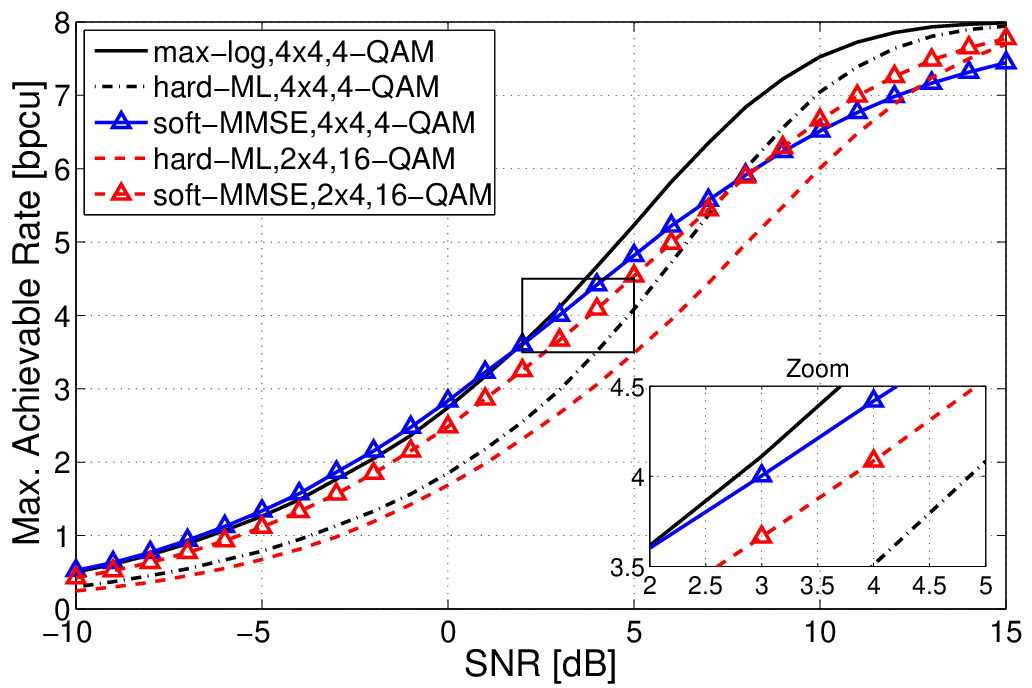

Soft MMSE demodulation approaches BICM capacity and outperforms max-log at low rates, both in the ergodic and the quasi-static regime and for various system configurations (see also [31]). Moreover, soft MMSE is very attractive since it has the lowest complexity among all soft demodulators that we discussed. Therefore, soft MMSE demodulation is arguably the demodulator of choice when designing MIMO-BICM systems with outer codes of low to medium rate. Since soft ZF performs consistently poorer than soft MMSE at the same computational cost, there appears to be no reason to prefer soft ZF in practical implementations. The case for soft MMSE is particularly strong for asymmetric MIMO systems (i.e., ), where it performs close to BICM capacity for all rates. Fig. 12(a) compares a MIMO system using -QAM (system I) and a system using -QAM (system II), both using Gray labeling and achieving . Whereas at low rates soft MMSE demodulation performs better with system I than with system II, it is the other way around for high rates. For example, at bpcu system II requires dB less SNR than system I, in spite of using fewer active transmit antennas. This observation is of interest when designing MIMO-BICM systems with adaptive modulation and coding. Specifically, with soft MMSE demodulation system I is preferable below bpcu, whereas above bpcu it is advantageous to deactivate two transmit antennas and switch to the -QAM constellation (system II). We note that with max-log and hard ML demodulation, system II performs consistently worse than system I. The only regime where soft MMSE suffers from a noticeable performance loss is symmetric systems at high rates (both, in the ergodic and quasi-static scenario). In the high-rate regime, hard and soft SDR are the only low-complexity demodulation schemes that are able to achieve hard ML and max-log performance, respectively. These observations apply also in the case of imperfect CSI. This suggests that hard and soft SDR demodulation are preferable over hard ML and max-log demodulation. With perfect CSI, also LSD, bit-flipping demodulation, and soft -norm demodulation come reasonably close to max-log. The LSD has the additional advantage of being able to trade off performance for complexity reduction. Furthermore, note that for system I hard SDR demodulation (which approaches hard ML performance) outperforms most suboptimal soft demodulators for rates larger than bpcu.
The above discussion suggests that in order to achieve a given target information rate, it may be preferable to adapt the number of antennas and the symbol constellation in a system with a low-rate code and a low-complexity MMSE demodulator instead of using a high-rate code and a computationally expensive non-linear demodulator. Such a design approach has recently been advocated also in [60]. While RF complexity may be a limiting factor with respect to antenna number, increasing the constellation size is inexpensive. Fig. 12(b) compares soft MMSE and max-log for a MIMO system with Gray-labeled -QAM () and -QAM (). Below 3.5 bpcu, soft MMSE demodulation with 4-QAM is optimal; at higher rates, switching to -QAM allows the MMSE demodulator to perform within about dB of max-log with 4-QAM while increasing the soft-MMSE complexity only little.
In case of imperfect receiver CSI, the performance of all demodulators deteriorates significantly (see also [31]), i.e., all capacity curves are shifted to higher SNRs (depending on the amount of training). Demodulators that take the noise variance into account require somewhat more training. An exception is the LSD which can outperform max-log in case of poor channel and noise variance estimates [31].
We conclude that at low rates linear soft demodulation is generally preferable due to its very low computational complexity. At high rates non-linear demodulators perform better, even when they deliver hard rather than soft outputs. If complexity is not an issue, soft SDR demodulation is advantageous since it approaches max-log performance and is largely superior to all other demodulators over a wide range of system parameters and SNRs. A notable exception is the low-complexity SoftIC demodulator which for some system configurations has the potential to outperform soft SDR (and max-log) at low rates.
IX Conclusion
We provided a comprehensive performance assessment and comparison of soft and hard demodulators for non-iterative MIMO-BICM systems. Our comparison is based on the information-theoretic notion of system capacity, which can be interpreted as the maximum achievable rate of the equivalent “modulation” channel that comprises modulator, physical channel, and demodulator. As a performance measure, system capacity has the main advantage of being independent of any outer code. Extensive simulation results show that a universal demodulator performance ranking is not possible and that the demodulator performance can depend strongly on the rate (or equivalently the SNR) at which a system operates. In addition to ergodic capacity results, we investigated the non-ergodic fading scenario in terms of outage probability and -capacity and analyzed the robustness of certain demodulators under imperfect channel state information. Our observations provide new insights into the design of MIMO-BICM systems (i.e., choice of demodulator, number of antennas, and symbol constellation). Moreover, our approach sheds light on issues that have not been apparent in the previously prevailing BER performance comparisons for specific outer codes. For example, a key observation is that with low-rate outer codes soft MMSE is preferable over other demodulators since it has low complexity but close-to-optimal performance.
Appendix A Measuring Mutual Information
Evaluating the mutual information in (9) involves the conditional LLR distributions . We approximate these pdfs by histograms obtained via Monte Carlo simulations. To achieve a small bias and variance of the mutual information estimate, the number and the size of the histogram bins as well as the sample size need to be carefully balanced [48]. Instead of LLRs, we use the bit probabilities
Since the LLRs and are in one-to-one correspondence (cf. (2)), the mutual information of the equivalent modulation channel equals that of the channel characterized by the conditional pdf ; the latter has the advantage of being easier to approximate by a histogram with uniform bins. By performing Monte Carlo simulations in which code bits, the noise, and the channel are randomly generated, we obtain a histogram with bins which is characterized by the uniform bins , , and the associated conditional relative frequencies (i.e., the normalized number of probabilities lying in the th bin conditioned on ). The mutual information in (9) is then approximated as
| (26) |
The accuracy of this approximation depends i) on the number of histogram bins (this determines the discretization error) and ii) on the number of samples (code bits) used to estimate the histogram (this determines the bias and variance of and hence of ). Specifically, the bias and the variance of can be bounded as (see [48])
| (27) |
Here, is the mutual information of the discretized channel, i.e., equal to (26) but with replaced by . Hence, the bias in (27) quantifies the systematic error resulting from the empirical estimation of the histograms. We conclude that a large number of bins is advantageous in order to keep the discretization error small; in view of (27), this necessitates a significantly larger number of samples () in order to achieve a small estimation bias. Large simultaneously ensures a small estimation variance. The price paid for accurate capacity estimates is computational complexity.
To design and , we first evaluated the BICM capacity in (7) by direct numerical integration using the known pdfs in (5); then we estimated the same capacity via Monte Carlo simulations as described above using the optimum soft MAP demodulator and increasingly larger and until the result was close enough to the capacity obtained by direct evaluation. Specifically, with and the estimation error was on the order of over a large SNR range. These numbers were then used to estimate the mutual information for all other demodulators.
Acknowledgment
The authors thank Gottfried Lechner for kindly providing his LDPC decoder implementation.
References
- [1] P. Fertl, J. Jaldén, and G. Matz, “Capacity-based performance comparison of MIMO-BICM demodulators,” in Proc. IEEE SPAWC-2008, Recife, Brazil, July 2008, pp. 166–170.
- [2] G. Caire, G. Taricco, and E. Biglieri, “Bit-interleaved coded modulation,” IEEE Trans. Inf. Theory, vol. 44, no. 5, pp. 927–945, May 1998.
- [3] A. Guillén i Fàbregas, A. Martinez, and G. Caire, “Bit-Interleaved Coded Modulation,” Foundations and Trends in Communications and Information Theory, vol. 5, no. 1–2, pp. 1–153, 2008.
- [4] U. Wachsmann, R. F. H. Fischer, and J. B. Huber, “Multilevel codes: Theoretical concepts and practical design rules,” IEEE Trans. Inf. Theory, vol. 45, no. 5, pp. 1361–1391, July 1999.
- [5] E. Biglieri, G. Taricco, and E. Viterbo, “Bit-interleaved time-space codes for fading channels,” in Proc. Conf. on Information Sciences and Systems, Princeton, NJ, Mar. 2000, pp. WA 4.1–4.6.
- [6] A. Stefanov and T. M. Duman, “Turbo-coded modulation for systems with transmit and receive antenna diversity over block fading channels: System model, decoding approaches, and practical considerations,” IEEE J. Sel. Areas Comm., vol. 19, no. 5, pp. 958–968, May 2001.
- [7] S. H. Müller-Weinfurtner, “Coding approaches for multiple antenna transmission in fast fading and OFDM,” IEEE Trans. Signal Processing, vol. 50, no. 10, pp. 2442–2450, Oct. 2002.
- [8] J. Jaldén and B. Ottersten, “Parallel implementation of a soft output sphere decoder,” in Proc. 39th Asilomar Conf. Signals, Systems, Computers, Pacific Grove, CA, Oct./Nov. 2005, pp. 581– 585.
- [9] ——, “On the complexity of sphere decoding in digital communications,” IEEE Trans. Signal Processing, vol. 53, no. 4, pp. 1474–1484, Apr. 2005.
- [10] C. Studer, A. Burg, and H. Bölcskei, “Soft-output sphere decoding: Algorithms and VLSI implementation,” IEEE J. Sel. Areas Comm., vol. 26, no. 2, pp. 290–300, Feb. 2008.
- [11] A. Burg, M. Borgmann, M. Wenk, M. Zellweger, W. Fichtner, and H. Bölcskei, “VLSI implementation of MIMO detection using sphere decoding algorithm,” IEEE J. Solid-State Circuits, vol. 40, no. 7, pp. 1566–1577, July 2005.
- [12] D. Seethaler and H. Bölcskei, “Performance and complexity analysis of infinity-norm sphere-decoding,” IEEE Trans. Inf. Theory, vol. 56, no. 3, pp. 1085–1105, Mar. 2010.
- [13] W. K. Ma, T. N. Davidson, K. M. Wong, Z. Q. Luo, and P. C. Ching, “Quasi-maximum-likelihood multiuser detection using semidefinite relaxation with application to synchronous CDMA,” IEEE Trans. Signal Processing, vol. 50, no. 4, pp. 912–922, Apr. 2002.
- [14] B. Steingrimsson, Z.-Q. Luo, and K. M. Wong, “Soft quasi-maximum-likelihood detection for multiple-antenna wireless channels,” IEEE Trans. Signal Processing, vol. 51, no. 11, pp. 2710–2719, Nov. 2003.
- [15] B. M. Hochwald and S. ten Brink, “Achieving near-capacity on a multiple-antenna channel,” IEEE Trans. Inf. Theory, vol. 51, no. 3, pp. 389–399, Mar. 2003.
- [16] H. Yao and G. W. Wornell, “Lattice-reduction-aided detectors for MIMO communication systems,” in Proc. IEEE GLOBECOM-2002, vol. 1, Taipei, Taiwan, Nov. 2002, pp. 424–428.
- [17] D. Wübben, R. Böhnke, V. Kühn, and K. Kammeyer, “MMSE-based lattice-reduction for near-ML detection of MIMO systems,” in Proc. ITG Workshop on Smart Antennas 2004, Munich, Germany, Mar. 2004, pp. 106–113.
- [18] C. Windpassinger, L. H.-J. Lampe, and R. F. H. Fischer, “From lattice-reduction-aided detection towards maximum-likelihood detection in MIMO systems,” in Proc. Wireless, Optical Commun. Conf., Banff, AB, Canada, July 2003.
- [19] P. Silvola, K. Hooli, and M. Juntii, “Suboptimal soft-output MAP detector with lattice reduction,” IEEE Signal Processing Letters, vol. 13, no. 6, pp. 321–324, June 2006.
- [20] V. Ponnampalam, D. McNamara, A. Lillie, and M. Sandell, “On generating soft outputs for lattice-reduction-aided MIMO detection,” in Proc. IEEE ICC-07, Glasgow, UK, June 2007, pp. 4144–4149.
- [21] R. Wang and G. B. Giannakis, “Approaching MIMO channel capacity with soft detection based on hard sphere decoding,” IEEE Trans. Comm., vol. 54, no. 4, pp. 587–590, Apr. 2006.
- [22] M. Butler and I. Collings, “A zero-forcing approximate log-likelihood receiver for MIMO bit-interleaved coded modulation,” IEEE Commun. Letters, vol. 8, no. 2, pp. 105–107, Feb. 2004.
- [23] M. R. McKay and I. B. Collings, “Capacity and performance of MIMO-BICM with zero-forcing receivers,” IEEE Trans. Comm., vol. 53, no. 1, pp. 74–83, Jan. 2005.
- [24] I. B. Collings, M. R. G. Butler, and M. R. McKay, “Low complexity receiver design for MIMO bit-interleaved coded modulation,” in IEEE ISSTA-2004, Sydney, Australia, Aug.-Sep. 2004, pp. 12–16.
- [25] D. Seethaler, G. Matz, and F. Hlawatsch, “An efficient MMSE-based demodulator for MIMO bit-interleaved coded modulation,” in Proc. IEEE GLOBECOM-2004, vol. 4, Dallas, Texas, Dec. 2004, pp. 2455–2459.
- [26] W.-J. Choi, K.-W. Cheong, and J. Cioffi, “Iterative soft interference cancellation for multiple antenna systems,” in Proc. IEEE WCNC-2000, vol. 1, Chicago, IL, Sep. 2000, pp. 304–309.
- [27] A. Paulraj, R. U. Nabar, and D. Gore, Introduction to Space-Time Wireless Communications. Cambridge (UK): Cambridge Univ. Press, 2003.
- [28] P. W. Wolniansky, G. J. Foschini, G. D. Golden, and R. A. Valenzuela, “V-BLAST: An architecture for realizing very high data rates over the rich-scattering wireless channel,” in Proc. URSI Int. Symp. on Signals, Systems and Electronics, Pisa, Italy, Sep. 1998, pp. 295–300.
- [29] B. Hassibi, “A fast square-root implementation for BLAST,” in Proc. 34th Asilomar Conf. Signals, Systems, Computers, Pacific Grove, CA, Nov./Dec. 2000, pp. 1255–1259.
- [30] R. Böhnke, D. Wübben, V. Kühn, and K. D. Kammeyer, “Reduced complexity MMSE detection for BLAST architectures,” in Proc. IEEE GLOBECOM-2003, vol. 4, San Francisco, CA, Dec. 2003, pp. 2258–2262.
- [31] P. Fertl, J. Jaldén, and G. Matz, “Performance assessment of MIMO-BICM demodulators based on system capacity: Further results,” Vienna University of Technology, Austria, Technical Report #09-1, Oct. 2009. [Online]. Available: http://publik.tuwien.ac.at/files/PubDat_174303.pdf
- [32] E. Telatar, “Capacity of multi-antenna Gaussian channels,” European Trans. Telecomm., vol. 10, no. 6, pp. 585–596, Nov. 1999.
- [33] T. M. Cover and J. A. Thomas, Elements of Information Theory. New York: Wiley, 1991.
- [34] L. H.-J. Lampe, R. Schober, and R. F. H. Fischer, “Multilevel coding for mutliple-antenna transmission,” IEEE Trans. Wireless Comm., vol. 3, no. 1, pp. 203–208, Jan. 2004.
- [35] Z. Hong and B. L. Hughes, “Robust space-time trellis codes based on bit-interleaved coded modulation,” in Proc. CISS-01, vol. 2, Mar. 2001, pp. 665–670.
- [36] M. van Dijk, A. J. E. M. Janssen, and A. G. C. Koppelaar, “Correcting systematic mismatches in computed log-likelihood ratios,” Europ. Trans. Telecomm., vol. 14, no. 3, pp. 227–244, July 2003.
- [37] D. Tse and P. Viswanath, Fundamentals of Wireless Communication. Boston (MA): Cambridge University Press, 2005.
- [38] A. Lapidoth and P. Naryan, “Reliable communication under channel uncertainty,” IEEE Trans. Inf. Theory, vol. 44, no. 6, pp. 2148–2177, Oct. 1998.
- [39] N. Merhav, G. Kaplan, A. Lapidoth, and S. Shamai, “On information rates for mismatched decoders,” IEEE Trans. Inf. Theory, vol. 40, no. 6, pp. 1953–1967, Nov. 1994.
- [40] A. Martinez, A. Guillén i Fàbregas, G. Caire, and F. Willems, “Bit-interleaved coded modulation revisited: A mismatched decoding perspective,” in Proc. ISIT-2008, Toronta, Canada, July 2008, pp. 2337–2341.
- [41] J. Jaldén, P. Fertl, and G. Matz, “On the generalized mutual information of BICM systems with approximate demodulation,” in Proc. IEEE Information Theory Workshop, Cairo, Egypt, Jan. 2010, pp. 1–5.
- [42] A. Burg, M. Wenk, and W. Fichtner, “VLSI implementation of pipelined sphere decoding with early termination,” in Proc. EUSIPCO-2006, Florence, Italy, Sept. 2006.
- [43] S. Schwandter, P. Fertl, C. Novak, and G. Matz, “Log-likelihood ratio clipping in MIMO-BICM systems: Information geometric analysis and impact on system capacity,” in Proc. IEEE ICASSP-2009, Taipei, Taiwan, Apr. 2009, pp. 2433–2436.
- [44] C. Novak, P. Fertl, and G. Matz, “Quantization for soft-output demodulators in bit-interleaved coded modulation systems,” in Proc. IEEE ISIT-2009, Seoul, Korea, Jun./Jul. 2009, pp. 1070–1074.
- [45] C. Studer and H. Bölcskei, “Soft-input soft-output single tree-search sphere decoding,” IEEE Trans. Inf. Theory, vol. 56, no. 10, pp. 4827–4842, Oct. 2010.
- [46] T. T. Nguyen and L. Lampe, “Bit-interleaved coded modulation with mismatched decoding metrics,” IEEE Trans. Communications, to appear.
- [47] J. M. Cioffi, G. P. Dudevoir, M. V. Eyuboglu, and G. D. Forney, “MMSE decision-feedback equalizers and coding – Part I: Equalization results,” IEEE Trans. Commun., vol. 43, no. 10, pp. 2582–2594, Oct. 1995.
- [48] L. Paninski, “Estimation of entropy and mutual information,” Neural Comput., vol. 15, no. 6, pp. 1191–1253, June 2003.
- [49] T. J. Richardson and R. L. Urbanke, “The capacity of low-density parity check codes under message-passing decoding,” IEEE Trans. Inf. Theory, vol. 47, no. 2, pp. 599–618, Feb. 2001.
- [50] C. Michalke, E. Zimmermann, and G. Fettweis, “Linear MIMO receivers vs. tree search detection: A performance comparison overview,” in Proc. IEEE PIMRC-06, Helsinki, Finland, Sept. 2006, pp. 1–7.
- [51] M. Damen, H. El Gamal, and G. Caire, “On maximum-likelihood detection and the search for the closest lattice point,” IEEE Trans. Inf. Theory, vol. 49, no. 10, pp. 2389–2402, Oct. 2003.
- [52] A. K. Lenstra, H. W. Lenstra, Jr., and L. Lovász, “Factoring polynomials with rational coefficients,” Math. Ann., vol. 261, no. 4, pp. 515–534, Dec. 1982.
- [53] J. Jaldén, D. Seethaler, and G. Matz, “Worst- and average-case complexity of LLL lattice reduction in MIMO wireless systems,” in Proc. IEEE ICASSP-2008, Las Vegas, NV, Apr. 2008, pp. 2685–2688.
- [54] D. Wübben and D. Seethaler, “On the performance of lattice reduction schemes for MIMO data detection,” in Proc. Asilomar Conf. Signals, Systems, Computers, Pacific Grove, CA, USA, Nov. 2007, pp. 1534–1538.
- [55] P. H. Tan and L. K. Rasmussen, “The application of semidefinite programming for detection in CDMA,” IEEE J. Sel. Areas Comm., vol. 19, no. 8, pp. 1442–1449, Aug. 2001.
- [56] R. A. Horn and C. R. Johnson, Matrix Analysis. Cambridge (UK): Cambridge Univ. Press, 1999.
- [57] M. Biguesh and A. B. Gershman, “Training-based MIMO channel estimation: A study of estimator tradeoffs and optimal training signals,” IEEE Trans. Signal Processing, vol. 54, no. 3, pp. 884–893, Mar. 2006.
- [58] G. Taricco and E. Biglieri, “Space-time decoding with imperfect channel estimation,” IEEE Trans. Wireless Comm., vol. 4, no. 4, pp. 1874–1888, July 2005.
- [59] A. Hedayat and A. Nosratinia, “Outage and diversity of linear receivers in flat-fading MIMO channels,” IEEE Trans. Signal Processing, vol. 55, no. 12, pp. 5868–5873, Dec. 2007.
- [60] K. R. Kumar, G. Caire, and A. L. Moustakas, “Asymptotic performance of linear receivers in MIMO fading channels,” IEEE Trans. Inf. Theory, vol. 55, no. 10, pp. 4398–4418, Oct. 2009.