跳到论文正文
W Papers独立论文阅读器 arXiv:0903.2595 论文正文 计算阅读时间 · 0%
引用这篇论文根据当前论文元数据生成,正式投稿前建议核对。


License: arXiv.org perpetual non-exclusive license
arXiv:0903.2595v1 [math-ph] 16 Mar 2009

ITEP/TH-12/09

Introduction to Integral Discriminants

A.Morozov and Sh.Shakirov11 1 morozov@itep.ru; shakirov@itep.ru

ITEP, Moscow, Russia
MIPT, Dolgoprudny, Russia

ABSTRACT

The simplest partition function, associated with homogeneous symmetric forms SS of degree rr in nn variables, is integral discriminant Jn|r​(S)=∫e−S⁡(x1,…,xn)​d​x1​…​d​xnJ_{n|r}\big(S\big)=\int e^{-S(x_{1},\ldots,x_{n})}\ dx_{1}\ldots dx_{n}. Actually, SS-dependence remains the same if e−Se^{-S} in the integrand is substituted by arbitrary function f⁡(S)f(S), i.e. integral discriminant is a characteristic of the form SS itself, and not of the averaging procedure. The aim of the present paper is to calculate Jn|rJ_{n|r} in a number of non-Gaussian cases. Using Ward identities – linear differential equations, satisfied by integral discriminants – we calculate J2|3,J2|4,J2|5J_{2|3},J_{2|4},J_{2|5} and J3|3J_{3|3}. In all these examples, integral discriminant appears to be a generalized hypergeometric function. It depends on several S​L​(n)SL(n) invariants of SS, with essential singularities controlled by the ordinary algebraic discriminant of SS.

1 Introduction

Averaging with exponential weight

⟨ϕ⟩=∫ϕ⁡(x)​e−S⁡(x)​𝑑x\left<\phi\right>=\int\phi(x)e^{-S(x)}dx

is an important operation in statistical and quantum physics. Function S⁡(x)S(x), which determines the weight, is called action. The integration domain of xx-variables is a linear space, which is usually infinite dimensional in real physical applications: for example, a space of paths in quantum mechanics or a space of field configurations in quantum field theory. Infinite dimension of the space introduces additional complications: the integral is not always well-defined. For this reason, it is important first to study such integrals in finite dimension nn. After this is done, one can take a n→∞n\rightarrow\infty limit.

However, even in finite dimension nn, the averaging operation is not yet fully understood. Most studied are Gaussian integrals: that is, when SS is quadratic in xx-variables. The simplest Gaussian integral

⟨1⟩=∫e−Si​j​xi​xj​dn​x\left<1\right>=\int e^{-S_{ij}x_{i}x_{j}}d^{n}x

is easily calculated and expressed through an invariant quantity – determinant – e.g. by diagonalising SS:

∫e−Si​j​xi​xj​dn​x=∫e−λ1​x12−…−λn​xn2​dn​x=1λ1​…​λn​∫e−x12−…−xn2​dn​x∼1detS\int e^{-S_{ij}x_{i}x_{j}}d^{n}x=\int e^{-\lambda_{1}x_{1}^{2}-\ldots-\lambda_{n}x_{n}^{2}}\ d^{n}x=\dfrac{1}{\sqrt{\lambda_{1}\ldots\lambda_{n}}}\int e^{-x_{1}^{2}-\ldots-x_{n}^{2}}\ d^{n}x\sim\dfrac{1}{\sqrt{\det S}}

The integral which factors out is just an SS-independent constant, which can be finite or infinite depending on the contour of integration. Therefore, essential SS-dependence of this Gaussian integral is given by (detS)−1/2(\det S)^{-1/2}. Any other Gaussian integral – with non-homogeneous quadratic SS or non-trivial ϕ\phi – is equally easy, because we have enough freedom to transform quadratic SS to diagonal or any other desired form. The possibility of diagonalisation greatly simplifies calculations with matrices (tensors with two indices).

Unfortunately, such methods do not work when SS is cubic or higher degree. This can be seen already from dimension counting. The number of independent coefficients Si​j​kS_{ijk}, which is n​(n+1)​(n+2)/6n(n+1)(n+2)/6, exceeds the number n2−1n^{2}-1 of available S​L​(n)SL(n) transformations, so it is not generally possible to diagonalize a cubic action – the group S​L​(n)SL(n) is too small. That is why the integral

∫e−Si​j​k​xi​xj​xk​dn​x\int e^{-S_{ijk}x_{i}x_{j}x_{k}}d^{n}x

and its higher degree analogues

Jn|r=∫e−S⁡(x1,…,xn)​dn​x,S⁡(x1,…,xn)=Si1,…,ir​xi1​…​xir\displaystyle J_{n|r}=\int e^{-S(x_{1},\ldots,x_{n})}d^{n}x,\ \ \ \ S(x_{1},\ldots,x_{n})=S_{i_{1},\ldots,i_{r}}x_{i_{1}}\ldots x_{i_{r}} (1)

despite simply-looking, still remain terra incognita. In [1, 2] integral Jn|r​(S)J_{n|r}(S) was named the integral discriminant of SS, because in the simplest cases this integral is just a power of algebraic discriminant Dn|r​(S)D_{n|r}(S). For example, there is an inspiring formula for 3-forms in two variables

J2|3=∫e−(a​x3+b​x2​y+c​x​y2+d​y3)dxdy=(27a2d2−b2c2−18abcd+4ac3+4b3d)−1/6=(D2|3)−1/6J_{2|3}=\int e^{-\big(ax^{3}+bx^{2}y+cxy^{2}+dy^{3}\big)}dxdy=\big(27a^{2}d^{2}-b^{2}c^{2}-18abcd+4ac^{3}+4b^{3}d\big)^{-1/6}=\left(D_{2|3}\right)^{-1/6}

which shows that J2|3J_{2|3} and D2|3D_{2|3} are, indeed, related. However, when one goes to higher nn and rr, the relation gets more complicated: Dn|rD_{n|r} defines only the singularities of Jn|rJ_{n|r}, while non-singular behaviour is controlled by other algebraic invariants. Thus, theory of integral discriminants is closely connected to invariant theory [3] and can be viewed as one of the branches of non-linear algebra [2], [4] - [8].

It would be very interesting to find a closed formula for generic Jn|rJ_{n|r}, because it could provide exciting new tools in QFT, statistics and other fields where non-Gaussian averaging is used. In this paper, we make a step in this direction and find integral discriminants explicitly for 3-forms, 4-forms and 5-forms in two variables, and for 3-forms in three variables. Our results indicate an intriguing connection between integral discriminants (1) and special functions known as generalized hypergeometric functions [9].

2 Ward identities

When the action is non-quadratic, diagonalisation and similar linear-algebra tricks fail. To handle non-Gaussian integrals, one needs essentially different methods. One of such methods (actually originated in the context of quantum field theory) is to find a differential equation, satisfied by the integral as a function of its parameters, see [10, 11] for typical applications and references. If such differential equation exists, we call it Ward identity (even if it is not directly induced by a change of integration variables).

Since Ward identities play the central role in present paper, let us give a pair of simple examples to clarify this issue. An integral

F(a)=∫e−x2/2+axdxF(a)=\int e^{-x^{2}/2+ax}dx

satisfies a Ward identity

(a−∂∂a)​F​(a)=0\left(a-\dfrac{\partial}{\partial a}\right)F(a)=0

because

(a−∂∂a)F(a)=∫(a−x)e−x2/2+axdx=∫(∂∂xe−x2/2+ax)dx=0\left(a-\dfrac{\partial}{\partial a}\right)F(a)=\int(a-x)e^{-x^{2}/2+ax}dx=\int\left(\dfrac{\partial}{\partial x}\ e^{-x^{2}/2+ax}\right)dx=0

In contrast with diagonalisation, this method is perfectly generalisable to non-Gaussian integrals: say,

G(a)=∫e−x3/3+axdxG(a)=\int e^{-x^{3}/3+ax}dx

satisfies a Ward identity

(a−∂2∂a2)​G​(a)=0\left(a-\dfrac{\partial^{2}}{\partial a^{2}}\right)G(a)=0

because

(a−∂2∂a2)G(a)=∫(a−x2)e−x3/3+axdx=∫(∂∂xe−x3/3+ax)dx=0\left(a-\dfrac{\partial^{2}}{\partial a^{2}}\right)G(a)=\int(a-x^{2})e^{-x^{3}/3+ax}dx=\int\left(\dfrac{\partial}{\partial x}\ e^{-x^{3}/3+ax}\right)dx=0

In this way the problem of non-Gaussian integrals is reduced to another problem – of differential equations. This is a much easier problem, especially if differential equations are linear. In the first case we have

a​F​(a)=∂∂a​F​(a)⟹F⁡(a)=c⋅ea2/2aF(a)=\dfrac{\partial}{\partial a}F(a)\ \ \Longrightarrow\ \ F(a)=c\cdot e^{a^{2}/2}

while in the second case

a​G​(a)=∂2∂a2​G​(a)⟹G⁡(a)=c1⋅ Ai ​(a)+c2⋅ Bi ​(a)aG(a)=\dfrac{\partial^{2}}{\partial a^{2}}G(a)\ \ \Longrightarrow\ \ G(a)=c_{1}\cdot\mbox{ Ai }(a)+c_{2}\cdot\mbox{ Bi }(a)

where Ai and Bi are special functions – Airy functions of the first and second kind. Note that, there is only one linear independent solution in the Gaussian case, while in the non-Gaussian case there are two linear-independent solutions. This is because to correctly define an integral, one still needs to specify an integration contour. Different integration contours provide different solutions of the Ward identity.

This relationship between Ward identities and integration contours is quite important, so let us add more details. As the simplest option, the contour of integration in the integral

Refer to caption
Figure 1: Two, out of infinitely many, admissible contours of integration for the integral ∫e−x2/2+axdx\int e^{-x^{2}/2+ax}dx.
F(a)=∫Ce−x2/2+axdxF(a)=\int\limits_{C}e^{-x^{2}/2+ax}dx

can be chosen as C=real axisC=\mbox{real axis}. However, this choice is by no means unique. In fact, any other contour CC which asymptotically tends to the lines Arg ​z=0\mbox{Arg }z=0 and Arg ​z=π/2\mbox{Arg }z=\pi/2, is admissible. A contour CC is said to be admissible, if the integral over CC converges. A few admissible contours are shown at Fig. 1. Note that, to ensure vanishing of the integral of full derivative (and thus validity of Ward identities) we consider only closed contors – the contours at Fig. 1. are closed on the Riemann sphere, if the infinitely remote point is taken into account. Since Ward identity in this case is a differential equation of first order, all the contours give one and the same answer F⁡(a)=exp⁡(a2/2)F(a)=\exp\big(a^{2}/2\big) up to proportionality.

More interesting is the non-Gaussian integral

G(a)=∫Ce−x3/3+axdxG(a)=\int\limits_{C}e^{-x^{3}/3+ax}dx

Note that, the real axis is no longer an admissible contour, since exp⁡(−x3)\exp\big(-x^{3}\big) grows to infinity when x→−∞x\rightarrow-\infty. In this case, admissible is any contour CC which asymptotically tends to the lines Arg ​z=0,Arg ​z=2​π/3\mbox{Arg }z=0,\ \mbox{Arg }z=2\pi/3 and Arg ​z=4​π/3\mbox{Arg }z=4\pi/3. A few admissible contours are shown at Fig. 2. Again, to ensure vanishing of the integral of full derivative, we consider only closed contors. Since Ward identity is second order in this case, there are two essentially different integration contours, say, C1C_{1} and C2C_{2}. An integral over arbitrary contour – the general solution of the Ward identity – is given by linear combination

∫e−x3/3+axdx=c1∫C1e−x3/3+axdx+c2∫C2e−x3/3+axdx\int\limits e^{-x^{3}/3+ax}dx\ =\ c_{1}\ \int\limits_{C_{1}}e^{-x^{3}/3+ax}dx\ +\ c_{2}\ \int\limits_{C_{2}}e^{-x^{3}/3+ax}dx

To summarize the above examples, Ward identity is the main differential equation which governs all the contours at once. The choice of particular contour corresponds to the choice of particular solution of the Ward identity. For this reason, Ward identities are especially convenient to study of properties, which are invariant under change of integration contour. Additional details can be found in [10].

Refer to caption
Figure 2: Three, out of infinitely many, admissible contours of integration for the integral ∫e−x3/3+axdx\int e^{-x^{3}/3+ax}dx.

3 Integral Discriminants

Definition.

In this paper we study a specific class of non-Gaussian integrals: integral discriminants

Jn|r​(S)=∫e−S⁡(x1,x2,…,xn)​d​x1​…​d​xnJ_{n|r}\big(S\big)=\int e^{-S(x_{1},x_{2},\ldots,x_{n})}dx_{1}\ldots dx_{n}

associated with homogeneous symmetric rr-forms S⁡(x1,x2,…,xn)S(x_{1},x_{2},\ldots,x_{n}). There are two different notations for symmetric forms, which can be useful under different circumstances: tensor notation

S⁡(x1,x2,…,xn)=∑i1,i2,…,ir=1nSi1,i2,…,ir​xi1​xi2​…​xirS(x_{1},x_{2},\ldots,x_{n})=\sum\limits_{i_{1},i_{2},\ldots,i_{r}=1}^{n}S_{i_{1},i_{2},\ldots,i_{r}}x_{i_{1}}x_{i_{2}}\ldots x_{i_{r}}

and monomial notation

S⁡(x1,x2,…,xn)=∑a1+a2+…+an=rsa1,a2​…​an​x1a1​x2a2​…​xnanS(x_{1},x_{2},\ldots,x_{n})=\sum\limits_{a_{1}+a_{2}+\ldots+a_{n}=r}s_{a_{1},a_{2}\ldots a_{n}}x_{1}^{a_{1}}x_{2}^{a_{2}}\ldots x_{n}^{a_{n}}

To distinguish between these notations, we denote coefficients by capital and small letters, respectively. Note, that in tensor notation coefficients have rr indices, while in monomial notation they have nn indices.

The choice of contour.

Being non-Gaussian integrals, integral discriminants of course depend on the choice of integration contour. One has to remember, that not every contour is admissible: for given SS, only restricted set of contours is allowed. Say, for positive-definite quadratic forms SS admissible is any contour, which is asymptotically pure real (see the previous section, especially Fig. 1 and Fig. 2 for simple examples). At the same time for negative-definite quadratic forms admissible is any contour, which is asymptotically pure imaginary. In this paper, we do not describe the contour dependence explicitly. Instead, we concentrate on contour-independent properties of integral discriminants.

Independence on the form of action.

An important feature of integral discriminants, which is due to homogeneity of SS, is the possibility to substitute the function e−Se^{-S} under the integral with arbitrary function (or, better to say, arbitrary good function) f⁡(S)f(S):

∫e−S⁡(x1,…,xn)​d​x1​…​d​xn∼∫f⁡(S⁡(x1,…,xn))​d​x1​…​d​xn\displaystyle\int e^{-S(x_{1},\ldots,x_{n})}\ dx_{1}\ldots dx_{n}\sim\int f\Big(S(x_{1},\ldots,x_{n})\Big)\ dx_{1}\ldots dx_{n} (2)

Even before specifying the class of good functions, let us consider a simple illustration with f⁡(S)=e−S2f(S)=e^{-S^{2}}:

∫e−(Si​j​xi​xj)​dn​x=∫e−(λ1​x12+…+λn​xn2)​dn​x=1λ1​…​λn​∫e−(x12+…+xn2)​dn​x=constdetS\int e^{-\big(S_{ij}x_{i}x_{j}\big)}\ d^{n}x=\int e^{-\big(\lambda_{1}x_{1}^{2}+\ldots+\lambda_{n}x_{n}^{2}\big)}\ d^{n}x=\dfrac{1}{\sqrt{\lambda_{1}\ldots\lambda_{n}}}\int e^{-\big(x_{1}^{2}+\ldots+x_{n}^{2}\big)}\ d^{n}x=\dfrac{{\rm const}}{\sqrt{\det S}}
∫e−(Si​j​xi​xj)2​dn​x=∫e−(λ1​x12+…+λn​xn2)2​dn​x=1λ1​…​λn​∫e−(x12+…+xn2)2​dn​x=const′detS\int e^{-\big(S_{ij}x_{i}x_{j}\big)^{2}}\ d^{n}x=\int e^{-\big(\lambda_{1}x_{1}^{2}+\ldots+\lambda_{n}x_{n}^{2}\big)^{2}}\ d^{n}x=\dfrac{1}{\sqrt{\lambda_{1}\ldots\lambda_{n}}}\int e^{-\big(x_{1}^{2}+\ldots+x_{n}^{2}\big)^{2}}\ d^{n}x=\dfrac{{\rm const^{\prime}}}{\sqrt{\det S}}

To specify the class of good functions and prove (2), let us make a change of integration variables

x1=ρ,x2=ρz2,x3=ρz3,…,xn=ρznx_{1}=\rho,\ \ x_{2}=\rho z_{2},\ \ x_{3}=\rho z_{3},\ \ \ldots,x_{n}=\rho z_{n}

i.e. pass from homogeneous coordinates xix_{i} to non-homogeneous coordinates zi=xi/x1z_{i}=x_{i}/x_{1}. Then

∫e−S⁡(x1,x2,…,xn)​d​x1​…​d​xn=∫ρn−1​𝑑ρ​∫d​z2​…​d​zn​e−ρr​S​(1,z2,…,zn)=\int e^{-S(x_{1},x_{2},\ldots,x_{n})}\ dx_{1}\ldots dx_{n}=\int\rho^{n-1}d\rho\int dz_{2}\ldots dz_{n}\ e^{-\rho^{r}S(1,z_{2},\ldots,z_{n})}=
=(∫ρn−1​e−ρr​𝑑ρ)⋅∫d​z2​…​d​znS​(1,z2,…,zn)n/r=\left(\int\rho^{n-1}e^{-\rho^{r}}d\rho\right)\cdot\int\dfrac{dz_{2}\ldots dz_{n}}{S(1,z_{2},\ldots,z_{n})^{n/r}}

For the right hand side of (2) we have

∫f⁡(S⁡(x1,x2,…,xn))​d​x1​…​d​xn=∫ρn−1​𝑑ρ​∫d​z2​…​d​zn​f​(ρr​S​(1,z2,…,zn))=\int f\Big(S(x_{1},x_{2},\ldots,x_{n})\Big)\ dx_{1}\ldots dx_{n}=\int\rho^{n-1}d\rho\int dz_{2}\ldots dz_{n}\ f\Big(\rho^{r}S(1,z_{2},\ldots,z_{n})\Big)=
=(∫ρn−1​f​(ρr)​𝑑ρ)⋅∫d​z2​…​d​znS​(1,z2,…,zn)n/r=\left(\int\rho^{n-1}f\Big(\rho^{r}\Big)d\rho\right)\cdot\int\dfrac{dz_{2}\ldots dz_{n}}{S(1,z_{2},\ldots,z_{n})^{n/r}}

Both integrals over ρ\rho are just SS-independent constants. As one can see, (2) is valid, iff these integrals

∫ρn−1​e−ρr​𝑑ρand∫ρn−1​f​(ρr)​𝑑ρ\int\rho^{n-1}e^{-\rho^{r}}d\rho\ \ \ \ {\rm and}\ \ \ \ \int\rho^{n-1}f\Big(\rho^{r}\Big)d\rho

are finite over one and the same contour. This condition specifies the class of good functions f⁡(S)f(S). For example, all functions f⁡(S)=exp⁡(−Sk)f(S)=\exp\big(-S^{k}\big) for k>0k>0 fall into this class. Relation (2) is therefore proved. As a byproduct, we have obtained a non-homogeneous integral representation

Jn|r​(S)=const⋅∫d​z2​…​d​znS​(1,z2,…,zn)n/r\boxed{\begin{gathered}J_{n|r}\big(S\big)={\rm const}\cdot\int\dfrac{dz_{2}\ldots dz_{n}}{S(1,z_{2},\ldots,z_{n})^{n/r}}\end{gathered}} (3)

A useful complement to the definiton of integral discriminants, representation (3) highlights two properties, which were less evident in (1): the scaling dimension

Jn|r(λS)=λ−n/rJn|r(S)\displaystyle J_{n|r}\big(\lambda S\big)=\lambda^{-n/r}\ J_{n|r}\big(S\big) (4)

and the vertical symmetry

In|k​r​(Sk)∼Jn|r​(S)\displaystyle I_{n|kr}\big(S^{k}\big)\sim J_{n|r}\big(S\big) (5)

Ward identities.

We now turn to Ward identities, satisfied by integral discriminants with respect to their parameters. Let us introduce the correlation functions

⟨ϕ⁡(x1,…,xn)⟩=∫ϕ⁡(x1,…,xn)​e−S⁡(x1,x2,…,xn)​d​x1​…​d​xn\Big<\phi(x_{1},\ldots,x_{n})\Big>=\int\phi(x_{1},\ldots,x_{n})e^{-S(x_{1},x_{2},\ldots,x_{n})}\ dx_{1}\ldots dx_{n}

These correlation functions satisfy

∂∂sa1,…,an⟨ϕ(x1,…,xn)⟩=−⟨x1a1…xnanϕ(x1,…,xn)⟩\displaystyle\dfrac{\partial}{\partial s_{a_{1},\ldots,a_{n}}}\Big<\phi(x_{1},\ldots,x_{n})\Big>=-\Big<x_{1}^{a_{1}}\ldots x_{n}^{a_{n}}\phi(x_{1},\ldots,x_{n})\Big> (6)

and

∂∂sa1,…,an​∂∂sb1,…,bn⟨ϕ⁡(x1,…,xn)⟩=⟨x1a1+b1​…​xnan+bn​ϕ​(x1,…,xn)⟩\dfrac{\partial}{\partial s_{a_{1},\ldots,a_{n}}}\dfrac{\partial}{\partial s_{b_{1},\ldots,b_{n}}}\Big<\phi(x_{1},\ldots,x_{n})\Big>=\Big<x_{1}^{a_{1}+b_{1}}\ldots x_{n}^{a_{n}+b_{n}}\phi(x_{1},\ldots,x_{n})\Big>

The right hand side depends only on the sum of indices ai+bia_{i}+b_{i}, not on aia_{i} and bib_{i} separately. For this reason, correlation functions satisfy a system of homogeneous second order differential equations:

(∂∂sa→​∂∂sb→−∂∂sp→​∂∂sq→)⟨ϕ⁡(x1,…,xn)⟩=0,a→+b→=p→+q→\displaystyle\left(\dfrac{\partial}{\partial s_{\vec{a}}}\dfrac{\partial}{\partial s_{\vec{b}}}-\dfrac{\partial}{\partial s_{\vec{p}}}\dfrac{\partial}{\partial s_{\vec{q}}}\right)\Big<\phi(x_{1},\ldots,x_{n})\Big>=0,\ \ \ \ \ {\vec{a}}+{\vec{b}}={\vec{p}}+{\vec{q}} (7)

In particular, if we set ϕ⁡(x1,…,xn)=1\phi(x_{1},\ldots,x_{n})=1 we find that integral discriminant ⟨1⟩=Jn|r\Big<1\Big>=J_{n|r} satisfies Ward identities

(∂∂sa→​∂∂sb→−∂∂sp→​∂∂sq→)​Jn|r​(S)=0,a→+b→=p→+q→\boxed{\begin{gathered}\left(\dfrac{\partial}{\partial s_{\vec{a}}}\dfrac{\partial}{\partial s_{\vec{b}}}-\dfrac{\partial}{\partial s_{\vec{p}}}\dfrac{\partial}{\partial s_{\vec{q}}}\right)J_{n|r}\big(S\big)=0,\ \ \ \ \ {\vec{a}}+{\vec{b}}={\vec{p}}+{\vec{q}}\end{gathered}} (8)

These equations do not exhaust the set of all Ward identities: there are more. Notice that the differential operator in the left hand side of (8) annihilates not only the integral, but also the integrand:

(∂∂sa→​∂∂sb→−∂∂sp→​∂∂sq→)​e−S⁡(x1,x2,…,xn)=0,a→+b→=p→+q→\left(\dfrac{\partial}{\partial s_{\vec{a}}}\dfrac{\partial}{\partial s_{\vec{b}}}-\dfrac{\partial}{\partial s_{\vec{p}}}\dfrac{\partial}{\partial s_{\vec{q}}}\right)e^{-S(x_{1},x_{2},\ldots,x_{n})}=0,\ \ \ \ \ {\vec{a}}+{\vec{b}}={\vec{p}}+{\vec{q}}

and even

(∂∂sa→​∂∂sb→−∂∂sp→​∂∂sq→)​f​(S⁡(x1,…,xn))=0,a→+b→=p→+q→\left(\dfrac{\partial}{\partial s_{\vec{a}}}\dfrac{\partial}{\partial s_{\vec{b}}}-\dfrac{\partial}{\partial s_{\vec{p}}}\dfrac{\partial}{\partial s_{\vec{q}}}\right)f\Big(S(x_{1},\ldots,x_{n})\Big)=0,\ \ \ \ \ {\vec{a}}+{\vec{b}}={\vec{p}}+{\vec{q}}

which justifies (2) once again. Usually, Ward differential operators do not annihilate the integrand, they just transform the integrand into a full derivative (which implies vanishing of the integral over any closed contour). Differential operator in the left hand side of (8) is therefore too special; one can expect other Ward identities to exist. To find them, let us consider the most general vanishing correlator – an integral of full derivative

∫∂∂xi​(ϕ⁡(x1,…,xn)​e−S⁡(x1,x2,…,xn))​d​x1​…​d​xn=0\int\dfrac{\partial}{\partial x_{i}}\left(\phi(x_{1},\ldots,x_{n})e^{-S(x_{1},x_{2},\ldots,x_{n})}\right)\ dx_{1}\ldots dx_{n}=0

Taking the derivative, we obtain Ward identities for correlation functions:

⟨∂ϕ⁡(x1,…,xn)∂xi⟩=⟨ϕ⁡(x1,…,xn)​∂S⁡(x1,…,xn)∂xi⟩\displaystyle\Big<\dfrac{\partial\phi(x_{1},\ldots,x_{n})}{\partial x_{i}}\Big>=\Big<\phi(x_{1},\ldots,x_{n})\dfrac{\partial S(x_{1},\ldots,x_{n})}{\partial x_{i}}\Big> (9)

For now we are not interested in all correlation functions, only in the integral discriminant. We need to rewrite the equations (9) as differential equations on Jn|rJ_{n|r}. There are several ways to do this, the simplest way is to set ϕ⁡(x1,…,xn)=xj\phi(x_{1},\ldots,x_{n})=x_{j} and use the identity (6) to get rid of remaining correlators. Doing so, we obtain equations

(δi​j+ai​A^i​j)​Jn|r=0\boxed{\begin{gathered}\left(\delta_{ij}+a_{i}\ {\hat{A}}_{ij}\right)J_{n|r}=0\end{gathered}} (10)

where operators

A^i​j=∑a1+a2+…+an=rsa1​…​ai−1​…​aj+1​…​an​∂∂sa1​…​an\displaystyle{\hat{A}}_{ij}=\sum\limits_{a_{1}+a_{2}+\ldots+a_{n}=r}s_{a_{1}\ldots a_{i}-1\ldots a_{j}+1\ldots a_{n}}\dfrac{\partial}{\partial s_{a_{1}\ldots a_{n}}} (11)

form the G​L​(n)GL(n) algrebra:

A^i​j​A^k​l−A^k​l​A^i​j=A^i​l​δk​j−A^k​j​δi​l{\hat{A}}_{ij}{\hat{A}}_{kl}-{\hat{A}}_{kl}{\hat{A}}_{ij}={\hat{A}}_{il}\delta_{kj}-{\hat{A}}_{kj}\delta_{il}

Note also, that other choices of ϕ⁡(x1,…,xn)\phi(x_{1},\ldots,x_{n}) in (9) do not give new Ward identities: everything, that can be obtained in this way, will be equivalent to (10). We conclude that the complete set of Ward identities for Jn|rJ_{n|r} consists of equations (8) and (10).

S​L​(n)SL(n) invariance.

In solving these Ward identities we start from (10), because they are first order. In fact, equations (10) simply reflect the G​L​(n)GL(n)-covariance (= S​L​(n)SL(n) invariance + correct scaling) of the model. This becomes clear, if we separate the generators of G​L​(n)GL(n) into two parts: the dilatation (degree) operator

A^11+…+A^n​n{\hat{A}}_{11}+\ldots+{\hat{A}}_{nn}

and the other n2−1n^{2}-1 operators, which form a representation of S​L​(n)SL(n). The first relation implies

(A^11+…+A^n​n)​Jn|r=−nr​Jn|r\left({\hat{A}}_{11}+\ldots+{\hat{A}}_{nn}\right)J_{n|r}=-\dfrac{n}{r}\ J_{n|r}

which is nothing but the scaling dimension (4). The other n2−1n^{2}-1 relations imply, that Jn|rJ_{n|r} is S​L​(n)SL(n)-invariant function of SS. Thus, equations (10) are completely solved by any S​L​(n)SL(n)-invariant function of SS, which is in addition homogeneous in SS of degree −n/r-n/r. A natural question is: is there any simple description of such functions? Actually, the answer to this question is positive: any S​L​(n)SL(n)-invariant function can be uniqely represented as a function of the elementary invariants IkI_{k}

Jn|r=F⁡{Ik}J_{n|r}=F\big\{I_{k}\big\}

much in the same way as any S​L​(n)SL(n)-invariant function of a matrix AjiA^{i}_{j} can be uniquely represented as a function of elementary invariants tr​Ak{\rm tr}A^{k}. Unfortunately, in the case of symmetric tensors Si1,…,irS_{i_{1},\ldots,i_{r}} classification of these elementary invariants IkI_{k} is not that easy, as in the case of matrices. Since a symmetric tensor with rr indices is much more complicated, than a matrix with two indices, no explicit formula like Ik=tr​AkI_{k}={\rm tr}A^{k} is available. The study of properties of the elementary invariants IkI_{k}, of different kinds of explicit formulas and relations between them, is a classical branch of science known as invariant theory [3].

The number of S​L​(n)SL(n) invariants.

Given parameters nn and rr of the form SS, one can easily find the number of elementary invariants IkI_{k}, of which all other invariants are various functions. Indeed, the linear space of forms SS of type n|rn|r has dimension

dimSn|r=(n+r−1)!r!​(n−1)!\dim S_{n|r}=\dfrac{(n+r-1)!}{r!(n-1)!}

that is the number of independent coefficients of symmetric tensor Si1​…​irS_{i_{1}\ldots i_{r}}. The group S​L​(n)SL(n) acts on this space, dividing it into orbits. All forms, connected by S​L​(n)SL(n) transformations Si1​…​ir↦Si1​…​ir​Uj1i1​…​Ujnin,U∈S​L​(n)S_{i_{1}\ldots i_{r}}\mapsto S_{i_{1}\ldots i_{r}}U^{i_{1}}_{j_{1}}\ldots U^{i_{n}}_{j_{n}},\ \ \ U\in SL(n) belong to one orbit. Ward identities imply, that Jn|rJ_{n|r} does not depend on coordinates along the orbit (”angular” variables). It depends only on transverse coordinates which label orbits (”radial” variables). Simple counting of dimensions implies, that dimension of the space of orbits, i.e. the number of radial coordinates, equals to

dimSn|r−dimS​L​(n)=(n+r−1)!r!​(n−1)!−n2+1\dim S_{n|r}-\dim SL(n)=\dfrac{(n+r-1)!}{r!(n-1)!}-n^{2}+1

Several examples of these numbers are shown at Fig. 3.

r\n23456721111113125112136427204691162531341102217414642069186427876\begin{array}[]{c|ccccccc}r\backslash n&&2&3&4&5&6&7\\ \\ \hline\cr\\ 2&&1&1&1&1&1&1\\ \\ 3&&1&2&5&11&21&36\\ \\ 4&&2&7&20&46&91&162\\ \\ 5&&3&13&41&102&217&414\\ \\ 6&&4&20&69&186&427&876\\ \\ \end{array}

Figure 3: The number of functionally independent S​L​(n)SL(n) invariants IkI_{k} of a form of degree rr in nn variables.

The Gaussian case Jn|2J_{n|2}.

Note, however, that the case r=2r=2 (quadratic forms) is exceptional, because the dimension dimSn|2=n⁡(n+1)/2\dim S_{n|2}=n(n+1)/2 is less than the dimension dimS​L​(n)=n2−1\dim SL(n)=n^{2}-1. For this reason, the above dimension counting does not work in this (and only in this) case. Actually, as we know, the space of S​L​(n)SL(n) orbits on quadratic forms is one-dimensional, and the only invariant – the single coordinate on the space of orbits – is determinant detS\det S. Thus, determinant is the only variable Jn|2J_{n|2} can depend on:

Jn|2​(S)=F⁡(detS)J_{n|2}\big(S\big)=F\big(\det S\big)

The homogeneity condition states, that F⁡(λ​x)=F⁡(x)/λF\big(\lambda x\big)=F\big(x\big)/\sqrt{\lambda} and has a single solution F⁡(x)=1/xF(x)=1/\sqrt{x}. In this way we reproduce the well-known Gaussian integral

Jn|2​(S)=1detS\boxed{\begin{gathered}\ \ \ J_{n|2}\big(S\big)=\dfrac{1}{\sqrt{\det S}}\ \ \ \end{gathered}} (12)

We emphasize, that simplicity of this answer is due to simplicity of the space of orbits, i.e, due to the fact there is a single invariant in this case. For higher rr, there are many invariants (as many as shown at Fig. 3) and Jn|rJ_{n|r} is a non-trivial function of all of them. The problem is that it becomes impossible to find Jn|rJ_{n|r} from the homogeneity condition alone. The solution of this problem is provided by Ward identities: in addition to the homogeneity condition, integral discriminant satisfies relations (8) and this allows to find F​{Ik}F\big\{I_{k}\big\}.

Diagram technique for S​L​(n)SL(n) invariants.

To do actual computations with S​L​(n)SL(n) invariants, we will adopt a convenient diagram technique, which is described in [2]. According to [2], it is possible to represent tensors with kk indices as kk-valent vertices, with two types of indices – covariant and contravariant – represented by two types of lines. Contraction of indices is naturally represented as connection of these lines. To simplify the diagrams, we use solid lines for both covariant and contravariant indices. In this paper we use the following four elementary building blocks for diagrams: covariant tensor Si1​…​irS_{i_{1}\ldots i_{r}}, represented by a black rr-valent vertex

[Uncaptioned image]

contravariant tensor ∂∂Si1​…​ir\dfrac{\partial}{\partial S_{i_{1}\ldots i_{r}}}, represented by a black rr-valent vertex

[Uncaptioned image]

completely antisymmetric contravariant tensor ϵi1​…​in\epsilon^{i_{1}\ldots i_{n}}, represented by a white nn-valent vertex

[Uncaptioned image]

and completely antisymmetric covariant tensor ϵi1​…​in∗\epsilon^{*}_{i_{1}\ldots i_{n}}, represented by a white nn-valent vertex

[Uncaptioned image]

Tensors ϵi1​…​in\epsilon^{i_{1}\ldots i_{n}} and ϵi1​…​in∗\epsilon^{*}_{i_{1}\ldots i_{n}} are completely antisymmetric with respect to permutations of their indices, and, therefore, remain invariant under S​L​(n)SL(n) transformations:

ϵi1​…​in​Ui1j1​…​Uinjn=detU⋅ϵj1​…​jn=ϵj1​…​jn\epsilon^{i_{1}\ldots i_{n}}U^{j_{1}}_{i_{1}}\ldots U^{j_{n}}_{i_{n}}=\det U\cdot\epsilon^{j_{1}\ldots j_{n}}=\epsilon^{j_{1}\ldots j_{n}}
ϵi1​…​in∗​Uj1i1​…​Ujnin=detU⋅ϵj1​…​jn∗=ϵj1​…​jn∗\epsilon^{*}_{i_{1}\ldots i_{n}}U^{i_{1}}_{j_{1}}\ldots U^{i_{n}}_{j_{n}}=\det U\cdot\epsilon^{*}_{j_{1}\ldots j_{n}}=\epsilon^{*}_{j_{1}\ldots j_{n}}

where detU=1\det U=1, because U∈S​L​(n)U\in SL(n). For this reason, any diagram without free (uncontracted) indices, made of contravariant ϵ\epsilon-vertices and covariant SS-vertices, is automatically S​L​(n)SL(n)-invariant function of SS. Say, determinant of n×nn\times n matrix Si​jS_{ij} can be represented as a diagram at Fig. 4, with nn SS-vertices and two ϵ\epsilon-vertices. The other two types of vertices (∂/∂S\partial/\partial S and ϵ∗\epsilon^{*}) will be used to construct S​L​(n)SL(n)-invariant differential operators.

Refer to caption
Figure 4: Determinant of matrix Si​jS_{ij}, represented as a diagram of tensor contraction. Black 2-valent vertices represent tensor SS, white n-valent vertices represent tensor ϵ\epsilon.

Diagrams provide a convenient way to obtain S​L​(n)SL(n) invariants. In fact, any S​L​(n)SL(n)-invariant can be obtained in this way, but, unfortunately, not uniquely: absolutely different-looking diagrams can represent one and the same invariant. Trying to resolve this ambiguity, one typically faces the complicated problems of classification of diagrams and finding relations between diagrams. These problems will not be adressed (and even touched) in present paper. Our goal is different: to find an explicit answer for Jn|rJ_{n|r} in several non-Gaussian cases, using diagrams as a convenient tool. We now turn to accomplishing this goal.

3.1 The case of J2|3J_{2|3}

The simplest non-trivial (i.e. non-Gaussian) example is a 33-form in 22 variables, which can be written as

S⁡(x,y)=S111​x3+3​S112​x2​y+3​S122​x​y2+S222​y2S(x,y)=S_{111}x^{3}+3S_{112}x^{2}y+3S_{122}xy^{2}+S_{222}y^{2}

By dimension counting, there is only one elementary invariant I4I_{4} in this case, given by a diagram at Fig. 5.

Refer to caption
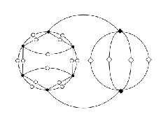
Figure 5: The degree 4 invariant I4I_{4} of a 3-form in 2 variables, represented as a diagram of tensor contraction. Black 3-valent vertices represent tensor SS, white 2-valent vertices represent tensor ϵ\epsilon.

The subscript ”4” stands for the degree of this invariant. In this paper we find it convenient to denote the elementary invariants of degree kk as IkI_{k}. It is straightforward to write the algebraic expression for the diagram:

I4=Si1​i2​i3​Sj1​j2​j3​Sk1​k2​k3​Sl1​l2​l3​ϵi1​j1​ϵi2​j2​ϵk1​l1​ϵk2​l2​ϵi3​k3​ϵj3​l3I_{4}=S_{i_{1}i_{2}i_{3}}S_{j_{1}j_{2}j_{3}}S_{k_{1}k_{2}k_{3}}S_{l_{1}l_{2}l_{3}}\epsilon^{i_{1}j_{1}}\epsilon^{i_{2}j_{2}}\epsilon^{k_{1}l_{1}}\epsilon^{k_{2}l_{2}}\epsilon^{i_{3}k_{3}}\epsilon^{j_{3}l_{3}}

Evaluating this sum, one gets the following explicit formula for I4I_{4}

I4=2​S1112​S2222−12​S111​S112​S122​S222+8​S111​S1223+8​S1123​S222−6​S1122​S1222I_{4}=2S_{111}^{2}S_{222}^{2}-12S_{111}S_{112}S_{122}S_{222}+8S_{111}S_{122}^{3}+8S_{112}^{3}S_{222}-6S_{112}^{2}S_{122}^{2}

which is nothing but the algebraic discriminant D2|3D_{2|3} of SS:

D2|3=I4\displaystyle D_{2|3}=I_{4} (13)

Since there is only one elementary invariant, the integral discriminant J2|3J_{2|3} must be a function of D2|3D_{2|3}:

J2|3​(S)=F⁡(I4)J_{2|3}\big(S\big)=F\big(I_{4}\big)

Thus, this case is similar to the Gaussian case. The homogeneity condition states, that F⁡(λ​x)=F⁡(x)/λ6F\big(\lambda x\big)=F\big(x\big)/\sqrt[6]{\lambda} and has a single solution F⁡(x)=1/x6F(x)=1/\sqrt[6]{x}. In this way we reproduce the formula from the Introduction:

J2|3(S)=I4−1/6\boxed{\begin{gathered}\ \ \ J_{2|3}\big(S\big)=I_{4}^{-1/6}\ \ \ \end{gathered}} (14)

In this case, one does not need to use the Ward identities (8): it is enough to use the homogeneity condition.

Refer to caption
Figure 6: The degree 2 invariant I2I_{2} of a 4-form in 2 variables, represented as a diagram of tensor contraction. Black 4-valent vertices represent tensor SS, white 2-valent vertices represent tensor ϵ\epsilon.
Refer to caption
Figure 7: The degree 3 invariant I3I_{3} of a 4-form in 2 variables, represented as a diagram of tensor contraction. Black 4-valent vertices represent tensor SS, white 2-valent vertices represent tensor ϵ\epsilon.

3.2 The case of J2|4J_{2|4}

The next-to-simplest example is a 44-form in 22 variables, which can be written as

S⁡(x,y)=S1111​x4+4​S1112​x3​y+6​S1122​x2​y2+4​S1222​x​y3+S2222​y4S(x,y)=S_{1111}x^{4}+4S_{1112}x^{3}y+6S_{1122}x^{2}y^{2}+4S_{1222}xy^{3}+S_{2222}y^{4}

Invariants.

By dimension counting, there are two elementary invariants in this case. They have relatively low degrees 22 and 33, denoted as I2I_{2} and I3I_{3} and given by diagrams at Fig. 6 and Fig. 7, respectively. Looking at the diagrams, it is straightforward to write algebraic expressions for I2,I3I_{2},I_{3}:

I2=Si1​i2​i3​i4​Sj1​j2​j3​j4​ϵi1​j1​ϵi2​j2​ϵi3​j3​ϵi4​j4I_{2}=S_{i_{1}i_{2}i_{3}i_{4}}S_{j_{1}j_{2}j_{3}j_{4}}\epsilon^{i_{1}j_{1}}\epsilon^{i_{2}j_{2}}\epsilon^{i_{3}j_{3}}\epsilon^{i_{4}j_{4}}
I3=Si1​i2​i3​i4​Sj1​j2​j3​j4​Sk1​k2​k3​k4​ϵi1​j1​ϵi2​j2​ϵi3​k1​ϵi4​k2​ϵj3​k3​ϵj4​k4I_{3}=S_{i_{1}i_{2}i_{3}i_{4}}S_{j_{1}j_{2}j_{3}j_{4}}S_{k_{1}k_{2}k_{3}k_{4}}\epsilon^{i_{1}j_{1}}\epsilon^{i_{2}j_{2}}\epsilon^{i_{3}k_{1}}\epsilon^{i_{4}k_{2}}\epsilon^{j_{3}k_{3}}\epsilon^{j_{4}k_{4}}

Evaluating these sums, one gets the following explicit formulas for I2,I3I_{2},I_{3}:

I2=2​S1111​S2222−8​S1112​S1222+6​S11222I_{2}=2S_{1111}S_{2222}-8S_{1112}S_{1222}+6S_{1122}^{2}
I3=6​S1111​S1122​S2222−6​S1111​S12222−6​S11122​S2222+12​S1112​S1122​S1222−6​S11223I_{3}=6S_{1111}S_{1122}S_{2222}-6S_{1111}S_{1222}^{2}-6S_{1112}^{2}S_{2222}+12S_{1112}S_{1122}S_{1222}-6S_{1122}^{3}

The algebraic discriminant D2|4D_{2|4}, just like any other S​L​(2)SL(2)-invariant function of SS, is a function of I2,I3I_{2},I_{3}:

D2|4=\displaystyle D_{2|4}= I23−6​I32=8​S11113​S22223−96​S11112​S1112​S1222​S22222−144​S11112​S11222​S22222+432​S11112​S1122​S12222​S2222\displaystyle\ I_{2}^{3}-6I_{3}^{2}\ =8S_{1111}^{3}S_{2222}^{3}-96S_{1111}^{2}S_{1112}S_{1222}S_{2222}^{2}-144S_{1111}^{2}S_{1122}^{2}S_{2222}^{2}+432S_{1111}^{2}S_{1122}S_{1222}^{2}S_{2222}
−216​S11112​S12224+432​S1111​S11122​S1122​S22222−48​S1111​S11122​S12222​S2222−1440​S1111​S1112​S11222​S1222​S2222\displaystyle-216S_{1111}^{2}S_{1222}^{4}+432S_{1111}S_{1112}^{2}S_{1122}S_{2222}^{2}-48S_{1111}S_{1112}^{2}S_{1222}^{2}S_{2222}-1440S_{1111}S_{1112}S_{1122}^{2}S_{1222}S_{2222}
+648​S1111​S11224​S2222+864​S1111​S1112​S1122​S12223+864​S11123​S1122​S1222​S2222+288​S11122​S11222​S12222\displaystyle+648S_{1111}S_{1122}^{4}S_{2222}+864S_{1111}S_{1112}S_{1122}S_{1222}^{3}+864S_{1112}^{3}S_{1122}S_{1222}S_{2222}+288S_{1112}^{2}S_{1122}^{2}S_{1222}^{2}
−432​S1111​S11223​S12222−216​S11124​S22222−512​S11123​S12223−432​S11122​S11223​S2222\displaystyle-432S_{1111}S_{1122}^{3}S_{1222}^{2}-216S_{1112}^{4}S_{2222}^{2}-512S_{1112}^{3}S_{1222}^{3}-432S_{1112}^{2}S_{1122}^{3}S_{2222} (15)

Integral discriminant.

Similarly, the integral discriminant is a function of I2,I3I_{2},I_{3}:

J2|4=F⁡(I2,I3)J_{2|4}=F\big(I_{2},I_{3}\big)

where the function FF is to be determined. The homogeneity condition does not allow to find FF unambigously, it constrains only the overall scaling factor, but not the non-trivial dependence on the ratio of invariants:

F(I2,I3)=I2−1/4G(I32I23)\displaystyle F\big(I_{2},I_{3}\big)=I_{2}^{-1/4}\ G\left(\dfrac{I_{3}^{2}}{I_{2}^{3}}\right) (16)

Ward identities.

To find the function G⁡(z)G(z) in this ansatz, we need to use the Ward identities (8). Applied to the present case of n=2,r=4n=2,r=4, the system (8) takes the form

(∂2∂s40​∂s22−∂2∂s31​∂s31)​J2|4=0(∂2∂s40​∂s13−∂2∂s31​∂s22)​J2|4=0(∂2∂s40​∂s04−∂2∂s31​∂s13)​J2|4=0(∂2∂s22​∂s22−∂2∂s31​∂s13)​J2|4=0\begin{array}[]{ccc}\left(\dfrac{\partial^{2}}{\partial s_{40}\partial s_{22}}-\dfrac{\partial^{2}}{\partial s_{31}\partial s_{31}}\right)J_{2|4}=0\\ \\ \left(\dfrac{\partial^{2}}{\partial s_{40}\partial s_{13}}-\dfrac{\partial^{2}}{\partial s_{31}\partial s_{22}}\right)J_{2|4}=0\\ \\ \left(\dfrac{\partial^{2}}{\partial s_{40}\partial s_{04}}-\dfrac{\partial^{2}}{\partial s_{31}\partial s_{13}}\right)J_{2|4}=0\\ \\ \left(\dfrac{\partial^{2}}{\partial s_{22}\partial s_{22}}-\dfrac{\partial^{2}}{\partial s_{31}\partial s_{13}}\right)J_{2|4}=0\\ \\ \end{array}

where ss-parameters and SS-parameters are related by

s40=S1111,s31=4​S1112,s22=6​S1122,s13=4​S1222,s04=S2222s_{40}=S_{1111},\ s_{31}=4S_{1112},\ s_{22}=6S_{1122},\ s_{13}=4S_{1222},\ s_{04}=S_{2222}

Particular equations in this system are, of course, not S​L​(2)SL(2) invariant. This is not convenient, since we are interested in S​L​(2)SL(2)-invariant solutions. Let us transform Ward identities into invariant form, using (16).

Invariant form of Ward identities.

Substituting the invariant anzatz (16) into the system, we obtain

(∂2∂s40​∂s22−∂2∂s31​∂s31)​J2|4=S1122​S2222−S122224​I29/4⋅((144​z2−24​z)​∂2G⁡(z)∂z2+(216​z−12)​∂G⁡(z)∂z+5​G​(z))(∂2∂s40​∂s13−∂2∂s31​∂s22)​J2|4=S1222​S1122−S1112​S22224​I29/4⋅((144​z2−24​z)​∂2G⁡(z)∂z2+(216​z−12)​∂G⁡(z)∂z+5​G​(z))(∂2∂s40​∂s04−∂2∂s31​∂s13)​J2|4=3​S1112​S1222−3​S112224​I29/4⋅((144​z2−24​z)​∂2G⁡(z)∂z2+(216​z−12)​∂G⁡(z)∂z+5​G​(z))(∂2∂s22​∂s22−∂2∂s31​∂s13)​J2|4=S1111​S2222−S1112​S122212​I29/4⋅((144​z2−24​z)​∂2G⁡(z)∂z2+(216​z−12)​∂G⁡(z)∂z+5​G​(z))\begin{array}[]{ccc}\\ \left(\dfrac{\partial^{2}}{\partial s_{40}\partial s_{22}}-\dfrac{\partial^{2}}{\partial s_{31}\partial s_{31}}\right)J_{2|4}=\dfrac{S_{1122}S_{2222}-S_{1222}^{2}}{4I_{2}^{9/4}}\cdot\left((144z^{2}-24z)\dfrac{\partial^{2}G(z)}{\partial z^{2}}+\left(216z-12\right)\dfrac{\partial G(z)}{\partial z}+5G(z)\right)\\ \\ \left(\dfrac{\partial^{2}}{\partial s_{40}\partial s_{13}}-\dfrac{\partial^{2}}{\partial s_{31}\partial s_{22}}\right)J_{2|4}=\dfrac{S_{1222}S_{1122}-S_{1112}S_{2222}}{4I_{2}^{9/4}}\cdot\left((144z^{2}-24z)\dfrac{\partial^{2}G(z)}{\partial z^{2}}+\left(216z-12\right)\dfrac{\partial G(z)}{\partial z}+5G(z)\right)\\ \\ \left(\dfrac{\partial^{2}}{\partial s_{40}\partial s_{04}}-\dfrac{\partial^{2}}{\partial s_{31}\partial s_{13}}\right)J_{2|4}=\dfrac{3S_{1112}S_{1222}-3S_{1122}^{2}}{4I_{2}^{9/4}}\cdot\left((144z^{2}-24z)\dfrac{\partial^{2}G(z)}{\partial z^{2}}+\left(216z-12\right)\dfrac{\partial G(z)}{\partial z}+5G(z)\right)\\ \\ \left(\dfrac{\partial^{2}}{\partial s_{22}\partial s_{22}}-\dfrac{\partial^{2}}{\partial s_{31}\partial s_{13}}\right)J_{2|4}=\dfrac{S_{1111}S_{2222}-S_{1112}S_{1222}}{12I_{2}^{9/4}}\cdot\left((144z^{2}-24z)\dfrac{\partial^{2}G(z)}{\partial z^{2}}+\left(216z-12\right)\dfrac{\partial G(z)}{\partial z}+5G(z)\right)\\ \\ \end{array}

where z=I32/I23z=I_{3}^{2}/I_{2}^{3}. These equations contain a common S​L​(2)SL(2) invariant factor. We conclude, that all the four expressions vanish, if and only if G⁡(z)G(z) satisfies the differential equation

(144​z2−24​z)​∂2G⁡(z)∂z2+(216​z−12)​∂G⁡(z)∂z+5​G​(z)=0\displaystyle(144z^{2}-24z)\dfrac{\partial^{2}G(z)}{\partial z^{2}}+\left(216z-12\right)\dfrac{\partial G(z)}{\partial z}+5G(z)=0 (17)

which is nothing but Gauss hypergeometric equation

t⁡(1−t)​∂2G⁡(t)∂t2+(c−(a+b+1)​t)​∂G⁡(t)∂t−a​b​G​(t)=0t(1-t)\dfrac{\partial^{2}G(t)}{\partial t^{2}}+\left(c-(a+b+1)t\right)\dfrac{\partial G(t)}{\partial t}-abG(t)=0

with a=1/12a=1/12, b=5/12b=5/12, c=1/2c=1/2 and t=6​zt=6z. This is the invariant form of n=2,r=4n=2,r=4 Ward identities.

Solution.

In terms of the Gauss hypergeometric function

F12​([a,b],[c],t)=∑k=0∞Γ⁡(a+k)Γ⁡(a)​Γ⁡(b+k)Γ⁡(b)​Γ⁡(c)Γ⁡(c+k)​tkk!=1+a​bc​t+a⁡(a+1)​b​(b+1)c⁡(c+1)​t22+…{}_{2}F_{1}\big(\left[a,b\right],\left[c\right],t\big)=\sum\limits_{k=0}^{\infty}\dfrac{\Gamma(a+k)}{\Gamma(a)}\dfrac{\Gamma(b+k)}{\Gamma(b)}\dfrac{\Gamma(c)}{\Gamma(c+k)}\dfrac{t^{k}}{k!}=1+\dfrac{ab}{c}t+\dfrac{a(a+1)b(b+1)}{c(c+1)}\dfrac{t^{2}}{2}+\ldots

the general solution of Gauss hypergeometric equation is given by

G⁡(t)=c1⋅F12​([a,b],[c],t)+c2⋅t1−c​F12​([a+1−c,b+1−c],[2−c],t)G(t)=c_{1}\cdot{}_{2}F_{1}\big(\left[a,b\right],\left[c\right],t\big)+c_{2}\cdot t^{1-c}\ {}_{2}F_{1}\big(\left[a+1-c,b+1-c\right],\left[2-c\right],t\big)

Consequently, the integral discriminant equals

J2|4(S)=c1⋅I2−1/42F1([112,512],[12],6​I32I23)+c2⋅I3I2−7/42F1([712,1112],[32],6​I32I23)\boxed{\begin{gathered}\ \ \ J_{2|4}\big(S\big)=c_{1}\cdot I_{2}^{-1/4}{}_{2}F_{1}\left(\left[\dfrac{1}{12},\dfrac{5}{12}\right],\left[\dfrac{1}{2}\right],\dfrac{6I_{3}^{2}}{I_{2}^{3}}\right)+c_{2}\cdot I_{3}I_{2}^{-7/4}{}_{2}F_{1}\left(\left[\dfrac{7}{12},\dfrac{11}{12}\right],\left[\dfrac{3}{2}\right],\dfrac{6I_{3}^{2}}{I_{2}^{3}}\right)\ \ \ \end{gathered}} (18)

where c1,2c_{1,2} are the two constants, parametrising the general solution of Ward identities. Particular solutions

J2|4(1)(S)=I2−1/4F12([112,512],[12],6​I32I23) and J2|4(2)(S)=I3I2−7/4F12([712,1112],[32],6​I32I23)J^{(1)}_{2|4}\big(S\big)=I_{2}^{-1/4}{}_{2}F_{1}\left(\left[\dfrac{1}{12},\dfrac{5}{12}\right],\left[\dfrac{1}{2}\right],\dfrac{6I_{3}^{2}}{I_{2}^{3}}\right)\ \ \ \mbox{ and }\ \ \ J^{(2)}_{2|4}\big(S\big)=I_{3}I_{2}^{-7/4}{}_{2}F_{1}\left(\left[\dfrac{7}{12},\dfrac{11}{12}\right],\left[\dfrac{3}{2}\right],\dfrac{6I_{3}^{2}}{I_{2}^{3}}\right)

are associated with different integration contours and can be called the first and the second branches of J2|4J_{2|4}.

Singularities.

Notice, that the point t=1t=1 corresponds to

6​I32I23=1\dfrac{6I_{3}^{2}}{I_{2}^{3}}=1

which is just the discriminant’s vanishing locus I23−6​I32=D2|4=0I_{2}^{3}-6I_{3}^{2}=D_{2|4}=0. This is interesting, because the point t=1t=1 is a singular point of the hypergeometric function F12{}_{2}F_{1}. However, there are two other suspicious points: hypergeometric function F12{}_{2}F_{1} can have singularities at t=0,1t=0,1 and ∞\infty. Let us study asymptotics of integral discriminants at these points, using the formulas

F12​([a,b],[c],t)=1+O⁡(t), when ​t→0\displaystyle{}_{2}F_{1}\left(\left[a,b\right],\left[c\right],t\right)=1+O(t),\ \ \ \ \mbox{ when }t\rightarrow 0 (19)
F12​([a,b],[a+b],1−t)=−Γ⁡(a+b)Γ⁡(a)​Γ​(b)​log⁡t+O⁡(t0), when ​t→0\displaystyle{}_{2}F_{1}\left(\left[a,b\right],\left[a+b\right],1-t\right)=-\dfrac{\Gamma(a+b)}{\Gamma(a)\Gamma(b)}\log t+O\big(t^{0}\big),\ \ \ \ \mbox{ when }t\rightarrow 0 (20)
F12​([a,b],[c],t)=\displaystyle{}_{2}F_{1}\left([a,b],[c],t\right)\ =\ t−a​Γ⁡(b−a)​Γ​(c)Γ⁡(b)​Γ​(c−a)⋅F12​([a,a−c+1],[a−b+1],1/t)+\displaystyle t^{-a}\dfrac{\Gamma(b-a)\Gamma(c)}{\Gamma(b)\Gamma(c-a)}\cdot{}_{2}F_{1}\left([a,a-c+1],[a-b+1],1/t\right)+\emph{}
t−b​Γ⁡(a−b)​Γ​(c)Γ⁡(a)​Γ​(c−b)⋅F12​([b,b−c+1],[b−a+1],1/t)\displaystyle t^{-b}\dfrac{\Gamma(a-b)\Gamma(c)}{\Gamma(a)\Gamma(c-b)}\cdot{}_{2}F_{1}\left([b,b-c+1],[b-a+1],1/t\right) (21)

which can be found in any reference book of hypergeometric functions (see, e.g. [12]). Using (19), we find

J2|4(1)(S)∼I2−1/4+O(t), when t→0J^{(1)}_{2|4}\big(S\big)\sim I_{2}^{-1/4}+O\big(t\big),\ \ \ \ \mbox{ when }t\rightarrow 0
J2|4(2)(S)∼I3I2−7/4+O(t), when t→0J^{(2)}_{2|4}\big(S\big)\sim I_{3}I_{2}^{-7/4}+O\big(t\big),\ \ \ \ \mbox{ when }t\rightarrow 0

Using (20), we find

J2|4(1)(S)∼−Γ⁡(1/2)Γ⁡(1/12)​Γ​(5/12)I2−1/4log(1−6​I32I23)+O(t0), when t→1J^{(1)}_{2|4}\big(S\big)\sim\dfrac{-\Gamma(1/2)}{\Gamma(1/12)\Gamma(5/12)}I_{2}^{-1/4}\log\big(1-\dfrac{6I_{3}^{2}}{I_{2}^{3}}\big)+O\big(t^{0}\big),\ \ \ \ \mbox{ when }t\rightarrow 1
J2|4(2)(S)∼−Γ⁡(3/2)Γ⁡(7/12)​Γ​(11/12)I3I2−7/4log(1−6​I32I23)+O(t0), when t→1J^{(2)}_{2|4}\big(S\big)\sim\dfrac{-\Gamma(3/2)}{\Gamma(7/12)\Gamma(11/12)}I_{3}I_{2}^{-7/4}\log\big(1-\dfrac{6I_{3}^{2}}{I_{2}^{3}}\big)+O\big(t^{0}\big),\ \ \ \ \mbox{ when }t\rightarrow 1

Using (19) and (21), we find

J2|4(1)(S)∼Γ⁡(1/2)​Γ​(1/3)Γ​(5/12)2(−6)−1/12I3−1/6+O(t−5/12), when t→∞J^{(1)}_{2|4}\big(S\big)\sim\dfrac{\Gamma(1/2)\Gamma(1/3)}{\Gamma(5/12)^{2}}(-6)^{-1/12}I_{3}^{-1/6}+O\big(t^{-5/12}\big),\ \ \ \ \mbox{ when }t\rightarrow\infty
J2|4(2)(S)∼Γ⁡(1/3)​Γ​(3/2)Γ​(11/12)2(−6)−7/12I3−1/6+O(t−11/12), when t→∞J^{(2)}_{2|4}\big(S\big)\sim\dfrac{\Gamma(1/3)\Gamma(3/2)}{\Gamma(11/12)^{2}}(-6)^{-7/12}I_{3}^{-1/6}+O\big(t^{-11/12}\big),\ \ \ \ \mbox{ when }t\rightarrow\infty

We can see from these results, that singularities of the integral discriminant J2|4J_{2|4} at finite values of I2,I3I_{2},I_{3} are completely controlled by the algebraic discriminant D2|4D_{2|4}. The singularity at discriminant locus is logarithmic. Other singularities, not related to the algebraic discriminant, are situated at infinite values of invariants: I2→∞I_{2}\rightarrow\infty (t→0t\rightarrow 0) and I3→∞I_{3}\rightarrow\infty (t→∞t\rightarrow\infty).

Hypergeometric integral.

Function F12{}_{2}F_{1} has an integral representation

F12​([a,b],[c],t)=Γ⁡(c)Γ⁡(b)​Γ​(c−b)⋅∫01d​s​sb−1​(1−s)c−b−1(1−s​t)a\displaystyle{}_{2}F_{1}\big(\left[a,b\right],\left[c\right],t\big)=\dfrac{\Gamma(c)}{\Gamma(b)\Gamma(c-b)}\cdot\int\limits_{0}^{1}ds\dfrac{s^{b-1}(1-s)^{c-b-1}}{(1-st)^{a}} (22)

which is a direct consequence of a simpler identity

Γ⁡(a)​Γ​(b)Γ⁡(a+b)=∫01d​s​sa−1​(1−s)b−1\displaystyle\dfrac{\Gamma(a)\Gamma(b)}{\Gamma(a+b)}=\int\limits_{0}^{1}ds\ s^{a-1}(1-s)^{b-1} (23)

For the integral discriminant, we obtain

J2|4​(S)=c1⋅∫01d​s​s−7/12(1−s)−11/12(I23−6​s​I32)1/12+c2​I3⋅∫01d​s​s−1/12(1−s)−5/12(I23−6​s​I32)7/12\boxed{\begin{gathered}J_{2|4}\big(S\big)=c_{1}\cdot\int\limits_{0}^{1}ds\ \dfrac{s^{-7/12}(1-s)^{-11/12}}{(I_{2}^{3}-6sI_{3}^{2})^{1/12}}+c_{2}I_{3}\cdot\int\limits_{0}^{1}ds\ \dfrac{s^{-1/12}(1-s)^{-5/12}}{(I_{2}^{3}-6sI_{3}^{2})^{7/12}}\end{gathered}} (24)

Hypergeometric functions with different values of parameters a,ba,b and cc are related by various ”modular” transformations of the variable tt and the integration variable ss, which leave the boundary region (two points 0 and 1) intact. Such transformations were first found and studied by Euler, therefore they are known as Euler hypergeometric transformations. Say, transformation t↦t,s↦1−st\mapsto t,\ s\mapsto 1-s gives rise to a relation

F12​([a,b],[c],t)=(1−t)−a⋅F12​([a,c−b],[c],tt−1)\displaystyle{}_{2}F_{1}\left(\left[a,b\right],\left[c\right],t\right)=(1-t)^{-a}\cdot{}_{2}F_{1}\left(\left[a,c-b\right],\left[c\right],\dfrac{t}{t-1}\right) (25)

After this transformation, J2|4J_{2|4} takes form

J2|4(1)(S)=(D2|4)−1/12F12([112,112],[12],−6​I32D2|4)J^{(1)}_{2|4}\big(S\big)=\left(D_{2|4}\right)^{-1/12}{}_{2}F_{1}\left(\left[\dfrac{1}{12},\dfrac{1}{12}\right],\left[\dfrac{1}{2}\right],-\dfrac{6I_{3}^{2}}{D_{2|4}}\right)
J2|4(2)(S)=I3(D2|4)−7/12F12([712,712],[32],−6​I32D2|4)J^{(2)}_{2|4}\big(S\big)=I_{3}\left(D_{2|4}\right)^{-7/12}{}_{2}F_{1}\left(\left[\dfrac{7}{12},\dfrac{7}{12}\right],\left[\dfrac{3}{2}\right],-\dfrac{6I_{3}^{2}}{D_{2|4}}\right)

In this way the hypergeometric integral (24) allows to recast J2|4J_{2|4} in various forms and establish relations between them. Therefore, (24) is a useful and important representation. We emphasise, that the relation of integral ∫e−S⁡(x,y)​𝑑x​𝑑y\int e^{-S(x,y)}dxdy to hypergeometric integrals (24) is not a priori expected: these integrals look very different, even from the point of view of variables they depend on.

Vertical symmetry.

To finish this section, let us check the vertical symmetry between J2|2J_{2|2} and J2|4J_{2|4}:

J2|4​((a​x2+b​x​y+c​y2)2)∼J2|2​(a​x2+b​x​y+c​y2)J_{2|4}\Big((ax^{2}+bxy+cy^{2})^{2}\Big)\sim J_{2|2}\Big(ax^{2}+bxy+cy^{2}\Big)

Setting S⁡(x,y)=(a​x2+b​x​y+c​y2)2S(x,y)=(ax^{2}+bxy+cy^{2})^{2} we obtain the coefficients

S1111=a2,S1112=12​a​b,S1122=13​a​c+16​b2,S1222=12​b​c,S2222=c2\begin{array}[]{ccc}S_{1111}=a^{2},\ \ S_{1112}=\dfrac{1}{2}ab,\ \ S_{1122}=\dfrac{1}{3}ac+\dfrac{1}{6}b^{2},\ \ S_{1222}=\dfrac{1}{2}bc,\ \ S_{2222}=c^{2}\\ \end{array}

and the invariants

I2=16​(b2−4​a​c)2,I3=136​(b2−4​a​c)3\begin{array}[]{ccc}I_{2}=\dfrac{1}{6}(b^{2}-4ac)^{2},\ \ I_{3}=\dfrac{1}{36}(b^{2}-4ac)^{3}\\ \end{array}

Substituting them into (18), we find

J2|4(1)​(S)=A(1)b2−4​a​cJ2|4(2)​(S)=A(2)b2−4​a​c\begin{array}[]{ccc}J^{(1)}_{2|4}\big(S\big)=\dfrac{A^{(1)}}{\sqrt{b^{2}-4ac}}\\ \\ J^{(2)}_{2|4}\big(S\big)=\dfrac{A^{(2)}}{\sqrt{b^{2}-4ac}}\\ \end{array}

where the constants of proportionality

A(1)=6−1/4⋅2F1([112,512],[12],1)∼−6−1/4Γ⁡(1/2)Γ⁡(1/12)​Γ​(5/12)log0∼∞A(2)=6+1/4⋅2F1([712,1112],[32],1)∼−6+1/4Γ⁡(3/2)Γ⁡(7/12)​Γ​(11/12)log0∼∞\begin{array}[]{ccc}A^{(1)}=6^{-1/4}\cdot{}_{2}F_{1}\left(\left[\dfrac{1}{12},\dfrac{5}{12}\right],\left[\dfrac{1}{2}\right],1\right)\sim-6^{-1/4}\dfrac{\Gamma(1/2)}{\Gamma(1/12)\Gamma(5/12)}\log 0\sim\infty\\ \\ A^{(2)}=6^{+1/4}\cdot{}_{2}F_{1}\left(\left[\dfrac{7}{12},\dfrac{11}{12}\right],\left[\dfrac{3}{2}\right],1\right)\sim-6^{+1/4}\dfrac{\Gamma(3/2)}{\Gamma(7/12)\Gamma(11/12)}\log 0\sim\infty\\ \end{array}

are independent of a,b,ca,b,c – as prescribed by the vertical symmetry – but infinite. Only their linear combination

(6+1/4Γ⁡(3/2)Γ⁡(7/12)​Γ​(11/12))A(1)−(6−1/4Γ⁡(1/2)Γ⁡(1/12)​Γ​(5/12))A(2)= finite number =−12\left(6^{+1/4}\dfrac{\Gamma(3/2)}{\Gamma(7/12)\Gamma(11/12)}\right)A^{(1)}-\left(6^{-1/4}\dfrac{\Gamma(1/2)}{\Gamma(1/12)\Gamma(5/12)}\right)A^{(2)}=\mbox{ finite number }=-\dfrac{1}{2}

is finite – logarithmic divergencies cancel out. Actually, it is expectable that only one linear combination of solutions stays finite. This is because not every contour, admissible for J2|4J_{2|4}, is admissible for J2|2J_{2|2}. Admissible contours for J2|4J_{2|4} approach infinity from 4 different directions, where the 4-form (a​x2+b​x​y+c​y2)2(ax^{2}+bxy+cy^{2})^{2} takes real positive values. Only two of these directions are appropriate for J2|2J_{2|2} – those, where the 2-form a​x2+b​x​y+c​y2ax^{2}+bxy+cy^{2} takes real positive values. One linear combination of branches corresponds to admissible contours, while the orthogonal linear combination corresponds to other contours. That is why both branches are singular at t→1t\rightarrow 1, but certain linear combination of branches is regular at t=1t=1. Note, that nothing similar happens at non-discriminantal singularities: at t→0t\rightarrow 0 and t→∞t\rightarrow\infty no linear combination of branches stays regular.

Refer to caption
Figure 8: The degree 4 invariant I4I_{4} of a 5-form in 2 variables, represented as a diagram of tensor contraction. Black 5-valent vertices represent tensor SS, white 2-valent vertices represent tensor ϵ\epsilon.

3.3 The case of J2|5J_{2|5}

Our third example is a 55-form in 22 variables, which can be written as

S⁡(x,y)=S11111​x5+5​S11112​x4​y+10​S11122​x3​y2+10​S11222​x2​y3+5​S12222​x​y4+S22222​y5S(x,y)=S_{11111}x^{5}+5S_{11112}x^{4}y+10S_{11122}x^{3}y^{2}+10S_{11222}x^{2}y^{3}+5S_{12222}xy^{4}+S_{22222}y^{5}

Invariants.

By dimension counting, there are three elementary invariants in this case. They have degrees 44, 88 and 1212, denoted as I4I_{4}, I8I_{8} and I12I_{12} and given by diagrams at Fig. 8, Fig. 9 and Fig. 10. Looking at the diagrams, it is straightforward to write an expression for I4I_{4}

I4=Si1​i2​i3​i4​i5​Sj1​j2​j3​j4​j5​Sk1​k2​k3​k4​k5​Sl1​l2​l3​l4​l5​ϵi1​j1​ϵi2​j2​ϵi3​j3​ϵi4​k4​ϵi5​k5​ϵj4​l4​ϵj5​l5​ϵk1​l1​ϵk2​l2​ϵk3​l3I_{4}=S_{i_{1}i_{2}i_{3}i_{4}i_{5}}S_{j_{1}j_{2}j_{3}j_{4}j_{5}}S_{k_{1}k_{2}k_{3}k_{4}k_{5}}S_{l_{1}l_{2}l_{3}l_{4}l_{5}}\epsilon^{i_{1}j_{1}}\epsilon^{i_{2}j_{2}}\epsilon^{i_{3}j_{3}}\epsilon^{i_{4}k_{4}}\epsilon^{i_{5}k_{5}}\epsilon^{j_{4}l_{4}}\epsilon^{j_{5}l_{5}}\epsilon^{k_{1}l_{1}}\epsilon^{k_{2}l_{2}}\epsilon^{k_{3}l_{3}}

and equally straightforward to write expressions for I8,I12I_{8},I_{12}. Evaluating the contraction, one gets a formula

I4=\displaystyle I_{4}\ =\ 2​S111112​S222222−20​S11111​S11112​S12222​S22222+8​S11111​S11122​S11222​S22222+\displaystyle 2S_{11111}^{2}S_{22222}^{2}-20S_{11111}S_{11112}S_{12222}S_{22222}+8S_{11111}S_{11122}S_{11222}S_{22222}+\emph{}
32​S11111​S11122​S122222−24​S11111​S112222​S12222+32​S111122​S11222​S22222+18​S111122​S122222−\displaystyle 32S_{11111}S_{11122}S_{12222}^{2}-24S_{11111}S_{11222}^{2}S_{12222}+32S_{11112}^{2}S_{11222}S_{22222}+18S_{11112}^{2}S_{12222}^{2}-\emph{}
24​S11112​S111222​S22222−152​S11112​S11122​S11222​S12222+96​S11112​S112223+96​S111223​S12222−64​S111222​S112222\displaystyle 24S_{11112}S_{11122}^{2}S_{22222}-152S_{11112}S_{11122}S_{11222}S_{12222}+96S_{11112}S_{11222}^{3}+96S_{11122}^{3}S_{12222}-64S_{11122}^{2}S_{11222}^{2}

and similar formulas for I8,I12I_{8},I_{12} – they are quite lengthy and we do not present them here. The algebraic discriminant D2|5D_{2|5}, just like any other S​L​(2)SL(2)-invariant function of SS, is a function of I4,I8,I12I_{4},I_{8},I_{12}:

D2|5=I42−64​I8\displaystyle D_{2|5}=I_{4}^{2}-64I_{8} (26)

Integral discriminant.

Similarly, the integral discriminant is a function of I4,I8,I12I_{4},I_{8},I_{12}:

J2|5=F⁡(I4,I8,I12)J_{2|5}=F\big(I_{4},I_{8},I_{12}\big)

where the function FF is to be determined. The homogeneity condition does not allow to find FF unambigously, it constrains only the overall scaling factor, but not the non-trivial dependence on the ratios of invariants:

Refer to caption
Figure 9: The degree 8 invariant I8I_{8} of a 5-form in 2 variables, represented as a diagram of tensor contraction. Black 5-valent vertices represent tensor SS, white 2-valent vertices represent tensor ϵ\epsilon.
F(I4,I8,I12)=I4−1/10G(I8I42,I12I43)\displaystyle F\big(I_{4},I_{8},I_{12}\big)=I_{4}^{-1/10}\ G\left(\dfrac{I_{8}}{I_{4}^{2}},\dfrac{I_{12}}{I_{4}^{3}}\right) (27)

To find the function G⁡(u,v)G(u,v) in this ansatz, we need to use the Ward identities (8).

Ward identities.

Applied to the present case of n=2,r=5n=2,r=5, the system (8) takes the form

(∂2∂s50​∂s32−∂2∂s41​∂s41)​J2|5=0(∂2∂s50​∂s23−∂2∂s41​∂s32)​J2|5=0(∂2∂s50​∂s14−∂2∂s41​∂s23)​J2|5=0​(∂2∂s32​∂s32−∂2∂s41​∂s23)​J2|5=0(∂2∂s50​∂s05−∂2∂s32​∂s23)​J2|5=0(∂2∂s41​∂s14−∂2∂s32​∂s23)​J2|5=0\begin{array}[]{ccc}\\ \left(\dfrac{\partial^{2}}{\partial s_{50}\partial s_{32}}-\dfrac{\partial^{2}}{\partial s_{41}\partial s_{41}}\right)J_{2|5}=0\\ \\ \left(\dfrac{\partial^{2}}{\partial s_{50}\partial s_{23}}-\dfrac{\partial^{2}}{\partial s_{41}\partial s_{32}}\right)J_{2|5}=0\\ \\ \left(\dfrac{\partial^{2}}{\partial s_{50}\partial s_{14}}-\dfrac{\partial^{2}}{\partial s_{41}\partial s_{23}}\right)J_{2|5}=0\\ \\ \end{array}\begin{array}[]{ccc}\\ \left(\dfrac{\partial^{2}}{\partial s_{32}\partial s_{32}}-\dfrac{\partial^{2}}{\partial s_{41}\partial s_{23}}\right)J_{2|5}=0\\ \\ \left(\dfrac{\partial^{2}}{\partial s_{50}\partial s_{05}}-\dfrac{\partial^{2}}{\partial s_{32}\partial s_{23}}\right)J_{2|5}=0\\ \\ \left(\dfrac{\partial^{2}}{\partial s_{41}\partial s_{14}}-\dfrac{\partial^{2}}{\partial s_{32}\partial s_{23}}\right)J_{2|5}=0\\ \\ \end{array}

where ss-parameters and SS-parameters are related by

s50=S11111,s41=5​S11112,s32=10​S11122,s23=10​S11222,s14=5​S12222,s05=S22222s_{50}=S_{11111},\ s_{41}=5S_{11112},\ s_{32}=10S_{11122},\ s_{23}=10S_{11222},\ s_{14}=5S_{12222},\ s_{05}=S_{22222}

Particular equations in this system are, of course, not S​L​(2)SL(2) invariant.

Refer to caption
Figure 10: The degree 12 invariant I12I_{12} of a 5-form in 2 variables, represented as a diagram of tensor contraction. Black 5-valent vertices represent tensor SS, white 2-valent vertices represent tensor ϵ\epsilon.

Invariant form of the Ward identities.

It is possible to deal with non-invariant equations (as we did in the previous section) but it is much more convenient to rewrite the above differential equations in S​L​(2)SL(2)-invariant form, by summing them with appropriate SS-dependent coefficients:

O^0=\displaystyle{\hat{O}}_{0}\ =\ (2​S11111​S12222−8​S11112​S11222+6​S111222)​(2​∂∂s50​∂∂s14−8​∂∂s41​∂∂s23+6​∂∂s32​∂∂s32)+\displaystyle(2S_{11111}S_{12222}-8S_{11112}S_{11222}+6S_{11122}^{2})\left(2\dfrac{\partial}{\partial s_{50}}\dfrac{\partial}{\partial s_{14}}-8\dfrac{\partial}{\partial s_{41}}\dfrac{\partial}{\partial s_{23}}+6\dfrac{\partial}{\partial s_{32}}\dfrac{\partial}{\partial s_{32}}\right)+\emph{}
2​(S11111​S22222−3​S11112​S12222+2​S11122​S11222)​(∂∂s05​∂∂s50−3​∂∂s41​∂∂s14+2​∂∂s32​∂∂s23)+\displaystyle 2(S_{11111}S_{22222}-3S_{11112}S_{12222}+2S_{11122}S_{11222})\left(\dfrac{\partial}{\partial s_{05}}\dfrac{\partial}{\partial s_{50}}-3\dfrac{\partial}{\partial s_{41}}\dfrac{\partial}{\partial s_{14}}+2\dfrac{\partial}{\partial s_{32}}\dfrac{\partial}{\partial s_{23}}\right)+\emph{}
(2​S11112​S22222−8​S11122​S12222+6​S112222)​(2​∂∂s41​∂∂s05−8​∂∂s32​∂∂s14+6​∂∂s23​∂∂s23)\displaystyle(2S_{11112}S_{22222}-8S_{11122}S_{12222}+6S_{11222}^{2})\left(2\dfrac{\partial}{\partial s_{41}}\dfrac{\partial}{\partial s_{05}}-8\dfrac{\partial}{\partial s_{32}}\dfrac{\partial}{\partial s_{14}}+6\dfrac{\partial}{\partial s_{23}}\dfrac{\partial}{\partial s_{23}}\right)

and

O^4=\displaystyle{\hat{O}}_{4}\ =\ P11​(S)​(2​∂∂s50​∂∂s14−8​∂∂s41​∂∂s23+6​∂∂s32​∂∂s32)+\displaystyle P_{11}\big(S\big)\ \left(2\dfrac{\partial}{\partial s_{50}}\dfrac{\partial}{\partial s_{14}}-8\dfrac{\partial}{\partial s_{41}}\dfrac{\partial}{\partial s_{23}}+6\dfrac{\partial}{\partial s_{32}}\dfrac{\partial}{\partial s_{32}}\right)+\emph{}
2​P12​(S)​(∂∂s05​∂∂s50−3​∂∂s41​∂∂s14+2​∂∂s32​∂∂s23)+\displaystyle 2P_{12}\big(S\big)\ \left(\dfrac{\partial}{\partial s_{05}}\dfrac{\partial}{\partial s_{50}}-3\dfrac{\partial}{\partial s_{41}}\dfrac{\partial}{\partial s_{14}}+2\dfrac{\partial}{\partial s_{32}}\dfrac{\partial}{\partial s_{23}}\right)+\emph{}
P22​(S)​(2​∂∂s41​∂∂s05−8​∂∂s32​∂∂s14+6​∂∂s23​∂∂s23)\displaystyle P_{22}\big(S\big)\ \left(2\dfrac{\partial}{\partial s_{41}}\dfrac{\partial}{\partial s_{05}}-8\dfrac{\partial}{\partial s_{32}}\dfrac{\partial}{\partial s_{14}}+6\dfrac{\partial}{\partial s_{23}}\dfrac{\partial}{\partial s_{23}}\right)

where PP is a quadratic form with coefficients

Pa​b​(S)=\displaystyle P_{ab}\big(S\big)\ =\ Sa​i2​i3​i4​i5​Sj1​j2​j3​j4​j5​Sk1​k2​k3​k4​k5​Sl1​l2​l3​l4​l5​Sm1​m2​m3​m4​m5​Ss1​s2​s3​s4​b\displaystyle S_{ai_{2}i_{3}i_{4}i_{5}}S_{j_{1}j_{2}j_{3}j_{4}j_{5}}S_{k_{1}k_{2}k_{3}k_{4}k_{5}}S_{l_{1}l_{2}l_{3}l_{4}l_{5}}S_{m_{1}m_{2}m_{3}m_{4}m_{5}}S_{s_{1}s_{2}s_{3}s_{4}b}
ϵi2​j2​ϵi3​j3​ϵi4​k4​ϵi5​k5​ϵk1​l1​ϵk2​l2​ϵj4​m4​ϵj5​m5​ϵm1​s1​ϵm2​s2​ϵl3​s3​ϵl4​s4​ϵj1​k3​ϵl5​m3\displaystyle\epsilon^{i_{2}j_{2}}\epsilon^{i_{3}j_{3}}\epsilon^{i_{4}k_{4}}\epsilon^{i_{5}k_{5}}\epsilon^{k_{1}l_{1}}\epsilon^{k_{2}l_{2}}\epsilon^{j_{4}m_{4}}\epsilon^{j_{5}m_{5}}\epsilon^{m_{1}s_{1}}\epsilon^{m_{2}s_{2}}\epsilon^{l_{3}s_{3}}\epsilon^{l_{4}s_{4}}\epsilon^{j_{1}k_{3}}\epsilon^{l_{5}m_{3}}\

Operators O^0{\hat{O}}_{0} and O^4{\hat{O}}_{4} are S​L​(2)SL(2)-invariant, simply because they are given by diagrams at Fig.11 and Fig.12. The subscripts ”0” and ”4” stand for the degrees of these operators. In analogy with invariants IkI_{k}, we denote the invariant differential operators of degree kk as O^k{\hat{O}}_{k}.

Refer to caption
Figure 11: Invariant differential operator O^0{\hat{O}}_{0} for the case 2|52|5, represented as a diagram of tensor contraction. Black 5-valent circles represent tensor SS, white 2-valent circles represent tensor ϵ\epsilon, black 5-valent rhombuses represent tensor ∂/∂S\partial/\partial S, white 2-valent rhombuses represent tensor ϵ∗\epsilon_{*}.
Refer to caption
Figure 12: Invariant differential operator O^4{\hat{O}}_{4} for the case 2|52|5, represented as a diagram of tensor contraction. Black 5-valent circles represent tensor SS, white 2-valent circles represent tensor ϵ\epsilon, black 5-valent rhombuses represent tensor ∂/∂S\partial/\partial S, white 2-valent rhombuses represent tensor ϵ∗\epsilon_{*}.

Of course, operators O^0{\hat{O}}_{0} and O^4{\hat{O}}_{4} are not unique – there are many other invariant differential operators, which annihilate J2|5J_{2|5}. All such operators contain an ϵ\epsilon-antisymmetrized combination of two derivatives ∂/∂S\partial/\partial S, which is exactly the structure of Ward identities. We do not study here the interesting problems of classification of these operators and finding relations between them, because O^0{\hat{O}}_{0} and O^4{\hat{O}}_{4} are quite enough to find J2|5J_{2|5}. Let us derive a useful formula for the action of second order operators

O^=∑α,βCα,β​∂∂Sα​∂∂Sβ\hat{O}=\sum\limits_{\alpha,\beta}C_{\alpha,\beta}\dfrac{\partial}{\partial S_{\alpha}}\dfrac{\partial}{\partial S_{\beta}}

By application of the chain rule, we obtain

O^​F​{Ik}=∑k∂F∂Ik​∑α,βCα,β​∂2Ik∂Sα​∂Sβ+∑k,m∂2F∂Ik​∂Im​∑α,βCα,β​∂Ik∂Sα​∂Im∂Sβ{\hat{O}}F\{I_{k}\}=\sum\limits_{k}\dfrac{\partial F}{\partial I_{k}}\sum\limits_{\alpha,\beta}C_{\alpha,\beta}\dfrac{\partial^{2}I_{k}}{\partial S_{\alpha}\partial S_{\beta}}+\sum\limits_{k,m}\dfrac{\partial^{2}F}{\partial I_{k}\partial I_{m}}\sum\limits_{\alpha,\beta}C_{\alpha,\beta}\dfrac{\partial I_{k}}{\partial S_{\alpha}}\dfrac{\partial I_{m}}{\partial S_{\beta}}

Since

∑α,βCα,β​∂2Ik∂Sα​∂Sβ=O^​Ik\sum\limits_{\alpha,\beta}C_{\alpha,\beta}\dfrac{\partial^{2}I_{k}}{\partial S_{\alpha}\partial S_{\beta}}={\hat{O}}I_{k}

and

∑α,β2​Cα,β​∂Ik∂Sα​∂Im∂Sβ=O^​(Ik​Im)−Ik​O^​Im−Im​O^​Ik\sum\limits_{\alpha,\beta}2C_{\alpha,\beta}\dfrac{\partial I_{k}}{\partial S_{\alpha}}\dfrac{\partial I_{m}}{\partial S_{\beta}}={\hat{O}}\big(I_{k}I_{m}\big)-I_{k}{\hat{O}}I_{m}-I_{m}{\hat{O}}I_{k}

we finally obtain an important formula:

O^​F​{Ik}=∑k∂F∂Ik​O^​Ik+12​∑k,m∂2F∂Ik​∂Im​[O^​(Ik​Im)−Ik​O^​Im−Im​O^​Ik]\boxed{\begin{gathered}\ \ \ {\hat{O}}F\{I_{k}\}=\sum\limits_{k}\dfrac{\partial F}{\partial I_{k}}{\hat{O}}I_{k}+\dfrac{1}{2}\sum\limits_{k,m}\dfrac{\partial^{2}F}{\partial I_{k}\partial I_{m}}\Big[{\hat{O}}\big(I_{k}I_{m}\big)-I_{k}{\hat{O}}I_{m}-I_{m}{\hat{O}}I_{k}\Big]\ \ \ \end{gathered}} (28)

As one can see, to describe the action of O^{\hat{O}}-operators on arbitrary invariant functions it suffices to calculate the action on all invariants IkI_{k} and all products Ik​ImI_{k}I_{m}. In the present case we have

O^0​(I4I8I12)=(26425​I4225​I42+29425​I81225​I4​I8+1625​I12){\hat{O}}_{0}\ \left(\begin{array}[]{ccc}\\ I_{4}\\ \\ I_{8}\\ \\ I_{12}\\ \\ \end{array}\right)=\left(\begin{array}[]{ccc}\\ \dfrac{264}{25}I_{4}\\ \\ \dfrac{2}{25}I_{4}^{2}+\dfrac{294}{25}I_{8}\\ \\ \dfrac{12}{25}I_{4}I_{8}+\dfrac{162}{5}I_{12}\\ \\ \end{array}\right)
O^0​(I42I4​I8I4​I12I4​I8I82I8​I12I4​I12I8​I12I122)=(92825​I42−38425​I8225​I43+116625​I4​I8+1925​I121225​I42​I8+14425​I82+179425​I4​I12225​I43+116625​I4​I8+1925​I12825​I42​I8+118825​I82+125​I4​I12925​I4​I82+1225​I42​I12+194425​I8​I121225​I42​I8+14425​I82+179425​I4​I12925​I4​I82+1225​I42​I12+194425​I8​I12−5425​I83+8425​I4​I8​I12+6845​I122){\hat{O}}_{0}\ \left(\begin{array}[]{ccc}\\ I_{4}^{2}&I_{4}I_{8}&I_{4}I_{12}\\ \\ I_{4}I_{8}&I_{8}^{2}&I_{8}I_{12}\\ \\ I_{4}I_{12}&I_{8}I_{12}&I_{12}^{2}\\ \\ \end{array}\right)=\left(\begin{array}[]{ccc}\\ \dfrac{928}{25}I_{4}^{2}-\dfrac{384}{25}I_{8}&\dfrac{2}{25}I_{4}^{3}+\dfrac{1166}{25}I_{4}I_{8}+\dfrac{192}{5}I_{12}&\dfrac{12}{25}I_{4}^{2}I_{8}+\dfrac{144}{25}I_{8}^{2}+\dfrac{1794}{25}I_{4}I_{12}\\ \\ \dfrac{2}{25}I_{4}^{3}+\dfrac{1166}{25}I_{4}I_{8}+\dfrac{192}{5}I_{12}&\dfrac{8}{25}I_{4}^{2}I_{8}+\dfrac{1188}{25}I_{8}^{2}+\dfrac{12}{5}I_{4}I_{12}&\dfrac{9}{25}I_{4}I_{8}^{2}+\dfrac{12}{25}I_{4}^{2}I_{12}+\dfrac{1944}{25}I_{8}I_{12}\\ \\ \dfrac{12}{25}I_{4}^{2}I_{8}+\dfrac{144}{25}I_{8}^{2}+\dfrac{1794}{25}I_{4}I_{12}&\dfrac{9}{25}I_{4}I_{8}^{2}+\dfrac{12}{25}I_{4}^{2}I_{12}+\dfrac{1944}{25}I_{8}I_{12}&-\dfrac{54}{25}I_{8}^{3}+\dfrac{84}{25}I_{4}I_{8}I_{12}+\dfrac{684}{5}I_{12}^{2}\\ \\ \end{array}\right)

and similarly for the second operator

O^4​(I4I8I12)=(−26425​I8−225​I4​I8+58825​I1236350​I82−15325​I4​I12){\hat{O}}_{4}\ \left(\begin{array}[]{ccc}\\ I_{4}\\ \\ I_{8}\\ \\ I_{12}\\ \\ \end{array}\right)=\left(\begin{array}[]{ccc}\\ -\dfrac{264}{25}I_{8}\\ \\ -\dfrac{2}{25}I_{4}I_{8}+\dfrac{588}{25}I_{12}\\ \\ \dfrac{363}{50}I_{8}^{2}-\dfrac{153}{25}I_{4}I_{12}\\ \\ \end{array}\right)
O^4​(I42I4​I8I4​I12I4​I8I82I8​I12I4​I12I8​I12I122)=(−92825​I4​I8−76825​I12−225​I42​I8−58425​I82+52425​I4​I1236350​I4​I82−15325​I42​I12−69625​I8​I12−225​I42​I8−58425​I82+52425​I4​I12125​I4​I82−2225​I42​I12+237625​I8​I1260350​I83−29125​I4​I8​I12+118825​I12236350​I4​I82−15325​I42​I12−69625​I8​I1260350​I83−29125​I4​I8​I12+118825​I1221295​I82​I12−60625​I4​I122){\hat{O}}_{4}\ \left(\begin{array}[]{ccc}\\ I_{4}^{2}&I_{4}I_{8}&I_{4}I_{12}\\ \\ I_{4}I_{8}&I_{8}^{2}&I_{8}I_{12}\\ \\ I_{4}I_{12}&I_{8}I_{12}&I_{12}^{2}\\ \\ \end{array}\right)=\left(\begin{array}[]{ccc}\\ -\dfrac{928}{25}I_{4}I_{8}-\dfrac{768}{25}I_{12}&-\dfrac{2}{25}I_{4}^{2}I_{8}-\dfrac{584}{25}I_{8}^{2}+\dfrac{524}{25}I_{4}I_{12}&\dfrac{363}{50}I_{4}I_{8}^{2}-\dfrac{153}{25}I_{4}^{2}I_{12}-\dfrac{696}{25}I_{8}I_{12}\\ \\ -\dfrac{2}{25}I_{4}^{2}I_{8}-\dfrac{584}{25}I_{8}^{2}+\dfrac{524}{25}I_{4}I_{12}&\dfrac{1}{25}I_{4}I_{8}^{2}-\dfrac{22}{25}I_{4}^{2}I_{12}+\dfrac{2376}{25}I_{8}I_{12}&\dfrac{603}{50}I_{8}^{3}-\dfrac{291}{25}I_{4}I_{8}I_{12}+\dfrac{1188}{25}I_{12}^{2}\\ \\ \dfrac{363}{50}I_{4}I_{8}^{2}-\dfrac{153}{25}I_{4}^{2}I_{12}-\dfrac{696}{25}I_{8}I_{12}&\dfrac{603}{50}I_{8}^{3}-\dfrac{291}{25}I_{4}I_{8}I_{12}+\dfrac{1188}{25}I_{12}^{2}&\dfrac{129}{5}I_{8}^{2}I_{12}-\dfrac{606}{25}I_{4}I_{12}^{2}\\ \\ \end{array}\right)

Applying (28), we obtain

O^0​F​(I4,I8,I12)=26425​I4​∂F∂I4+(225​I42+29425​I8)​∂F∂I8+(1225​I4​I8+1625​I12)​∂F∂I12{\hat{O}}_{0}F\big(I_{4},I_{8},I_{12}\big)=\dfrac{264}{25}I_{4}\dfrac{\partial F}{\partial I_{4}}+\left(\dfrac{2}{25}I_{4}^{2}+\dfrac{294}{25}I_{8}\right)\dfrac{\partial F}{\partial I_{8}}+\left(\dfrac{12}{25}I_{4}I_{8}+\dfrac{162}{5}I_{12}\right)\dfrac{\partial F}{\partial I_{12}}
+(8​I42−19225​I8)​∂2F∂I42+(225​I42​I8+12​I82+65​I4​I12)​∂2F∂I82+(−2725​I83+65​I4​I8​I12+36​I122)​∂2F∂I122+\left(8I_{4}^{2}-\dfrac{192}{25}I_{8}\right)\dfrac{\partial^{2}F}{\partial I_{4}^{2}}+\left(\dfrac{2}{25}I_{4}^{2}I_{8}+12I_{8}^{2}+\dfrac{6}{5}I_{4}I_{12}\right)\dfrac{\partial^{2}F}{\partial I_{8}^{2}}+\left(-\dfrac{27}{25}I_{8}^{3}+\dfrac{6}{5}I_{4}I_{8}I_{12}+36I_{12}^{2}\right)\dfrac{\partial^{2}F}{\partial I_{12}^{2}}
+(60825​I4​I8+1925​I12)​∂2F∂I4​∂I8+(14425​I82+1445​I4​I12)​∂2F∂I4​∂I12+(−325​I4​I82+25​I42​I12+1685​I8​I12)​∂2F∂I8​∂I12+\left(\dfrac{608}{25}I_{4}I_{8}+\dfrac{192}{5}I_{12}\right)\dfrac{\partial^{2}F}{\partial I_{4}\partial I_{8}}+\left(\dfrac{144}{25}I_{8}^{2}+\dfrac{144}{5}I_{4}I_{12}\right)\dfrac{\partial^{2}F}{\partial I_{4}\partial I_{12}}+\left(-\dfrac{3}{25}I_{4}I_{8}^{2}+\dfrac{2}{5}I_{4}^{2}I_{12}+\dfrac{168}{5}I_{8}I_{12}\right)\dfrac{\partial^{2}F}{\partial I_{8}\partial I_{12}}

and similarly for the second operator

O^4​F​(I4,I8,I12)=−26425​I8​∂F∂I4+(−225​I4​I8+58825​I12)​∂F∂I8+(36350​I82−15325​I4​I12)​∂F∂I12{\hat{O}}_{4}F\big(I_{4},I_{8},I_{12}\big)=-\dfrac{264}{25}I_{8}\dfrac{\partial F}{\partial I_{4}}+\left(-\dfrac{2}{25}I_{4}I_{8}+\dfrac{588}{25}I_{12}\right)\dfrac{\partial F}{\partial I_{8}}+\left(\dfrac{363}{50}I_{8}^{2}-\dfrac{153}{25}I_{4}I_{12}\right)\dfrac{\partial F}{\partial I_{12}}
+(−8​I4​I8−38425​I12)​∂2F∂I42+(110​I4​I82−1125​I42​I12+24​I8​I12)​∂2F∂I82+(14125​I82​I12−6​I4​I122)​∂2F∂I122+\left(-8I_{4}I_{8}-\dfrac{384}{25}I_{12}\right)\dfrac{\partial^{2}F}{\partial I_{4}^{2}}+\left(\dfrac{1}{10}I_{4}I_{8}^{2}-\dfrac{11}{25}I_{4}^{2}I_{12}+24I_{8}I_{12}\right)\dfrac{\partial^{2}F}{\partial I_{8}^{2}}+\left(\dfrac{141}{25}I_{8}^{2}I_{12}-6I_{4}I_{12}^{2}\right)\dfrac{\partial^{2}F}{\partial I_{12}^{2}}
+(−645​I82−6425​I4​I12)​∂2F∂I4​∂I8−43225​I8​I12​∂2F∂I4​∂I12+(245​I83−13625​I4​I8​I12+24​I122)​∂2F∂I8​∂I12+\left(-\dfrac{64}{5}I_{8}^{2}-\dfrac{64}{25}I_{4}I_{12}\right)\dfrac{\partial^{2}F}{\partial I_{4}\partial I_{8}}-\dfrac{432}{25}I_{8}I_{12}\dfrac{\partial^{2}F}{\partial I_{4}\partial I_{12}}+\left(\dfrac{24}{5}I_{8}^{3}-\dfrac{136}{25}I_{4}I_{8}I_{12}+24I_{12}^{2}\right)\dfrac{\partial^{2}F}{\partial I_{8}\partial I_{12}}

For the integral discriminant, both expressions vanish. Substituting the ansatz (27) and making the necessary algebraic transformations, we obtain two differential equations on the function G⁡(u,v)G(u,v): the first

50​(−1+64​u)​(u+6​u2+15​v)​∂2G∂u2+(75​u2+72000​v2+57600​v​u2+600​v​u+7200​u3−250​v)​∂2G∂u​∂v+\displaystyle 50(-1+64u)(u+6u^{2}+15v)\dfrac{\partial^{2}G}{\partial u^{2}}+(75u^{2}+72000v^{2}+57600vu^{2}+600vu+7200u^{3}-250v)\dfrac{\partial^{2}G}{\partial u\partial v}+\emph{}
(675​u3−13500​v2+10800​v​u2−750​v​u+43200​u​v2)​∂2G∂v2+(50400​v+30720​u2−50+5770​u)​∂G∂u+\displaystyle(675u^{3}-13500v^{2}+10800vu^{2}-750vu+43200uv^{2})\dfrac{\partial^{2}G}{\partial v^{2}}+(50400v+30720u^{2}-50+5770u)\dfrac{\partial G}{\partial u}+\emph{}
(−300​u+60480​v​u+11160​u2−7650​v)​∂G∂v+(528​u+110)​G=0\displaystyle(-300u+60480vu+11160u^{2}-7650v)\dfrac{\partial G}{\partial v}+(528u+110)G=0

and the second

25​(−1+64​u)​(5​u2+48​u​v−22​v)​∂2G∂u2+(230400​u​v2−39600​v2−6000​u3+28800​v​u2+6800​v​u)​∂2G∂u​∂v+\displaystyle 25(-1+64u)(5u^{2}+48uv-22v)\dfrac{\partial^{2}G}{\partial u^{2}}+(230400uv^{2}-39600v^{2}-6000u^{3}+28800vu^{2}+6800vu)\dfrac{\partial^{2}G}{\partial u\partial v}+\emph{}
(172800​v3+7500​v2+25200​u​v2−7050​v​u2)​∂2G∂v2+(−36120​v+4000​u2+122880​v​u+100​u)​∂G∂u+\displaystyle(172800v^{3}+7500v^{2}+25200uv^{2}-7050vu^{2})\dfrac{\partial^{2}G}{\partial v^{2}}+(-36120v+4000u^{2}+122880vu+100u)\dfrac{\partial G}{\partial u}+\emph{}
(241920​v2+19440​v​u−9075​u2+7650​v)​∂G∂v+(−220​u+2112​v)​G​(u,v)=0\displaystyle(241920v^{2}+19440vu-9075u^{2}+7650v)\dfrac{\partial G}{\partial v}+(-220u+2112v)G(u,v)=0

where u=I8/I42u=I_{8}/I_{4}^{2} and v=I12/I43v=I_{12}/I_{4}^{3}. These two linear differential equations in two variables constitute the invariant form of n=2,r=5n=2,r=5 Ward identities. Integral discriminant is found as the solution of this system.

Solution.

Having linear differential equations, it is easy to solve them in series: if one puts

G⁡(u,v)=∑i,jci​j​ui​vjG(u,v)=\sum\limits_{i,j}c_{ij}u^{i}v^{j}

then one finds, after some algebraic transformations,

ci​j=const⋅1i!​j!⋅16i​(1283)j⋅Γ⁡(310+i+j)​Γ​(110+2​i+3​j)​Γ​(110+j)Γ⁡(25+i+2​j)​Γ​(35+i+2​j)c_{ij}={\rm const}\cdot\dfrac{1}{i!j!}\cdot 16^{i}\left(\dfrac{128}{3}\right)^{j}\cdot\dfrac{\Gamma\left(\dfrac{3}{10}+i+j\right)\Gamma\left(\dfrac{1}{10}+2i+3j\right)\Gamma\left(\dfrac{1}{10}+j\right)}{\Gamma\left(\dfrac{2}{5}+i+2j\right)\Gamma\left(\dfrac{3}{5}+i+2j\right)}

i.e. there is unique series solution. In this way one obtains the first branch of the integral discriminant J2|5J_{2|5}:

J(1)2|5(S)=I4−1/10∑i,jΓ⁡(310+i+j)​Γ​(110+2​i+3​j)​Γ​(110+j)Γ⁡(25+i+2​j)​Γ​(35+i+2​j)⋅1i!​j!⋅(16​I8I42)i(128​I123​I43)j\!\boxed{\begin{gathered}J^{(1)}_{2|5}\big(S\big)=I_{4}^{-1/10}\sum\limits_{i,j}\dfrac{\Gamma\left(\dfrac{3}{10}+i+j\right)\Gamma\left(\dfrac{1}{10}+2i+3j\right)\Gamma\left(\dfrac{1}{10}+j\right)}{\Gamma\left(\dfrac{2}{5}+i+2j\right)\Gamma\left(\dfrac{3}{5}+i+2j\right)}\cdot\dfrac{1}{i!j!}\cdot\left(\dfrac{16I_{8}}{I_{4}^{2}}\right)^{i}\left(\dfrac{128I_{12}}{3I_{4}^{3}}\right)^{j}\end{gathered}} (29)

This answer is interesting: the function appears to be of generalised hypergeometric type [9], since its coefficients ci​jc_{ij} are ratios of Γ\Gamma-functions, depending on linear combinations of indices ii and jj. However, these series have a rather small convergence radius. Already the subsequence with i=ji=j behaves as

∑jΓ⁡(310+2​j)​Γ​(110+5​j)​Γ​(110+j)Γ⁡(25+3​j)​Γ​(35+3​j)​(2113​u​v)j∼∑j1j2​(213​5537​u​v)j\sum\limits_{j}\dfrac{\Gamma\left(\dfrac{3}{10}+2j\right)\Gamma\left(\dfrac{1}{10}+5j\right)\Gamma\left(\dfrac{1}{10}+j\right)}{\Gamma\left(\dfrac{2}{5}+3j\right)\Gamma\left(\dfrac{3}{5}+3j\right)}\left(\dfrac{2^{11}}{3}uv\right)^{j}\sim\sum\limits_{j}\dfrac{1}{j^{2}}\left(\dfrac{2^{13}5^{5}}{3^{7}}uv\right)^{j}

and diverges when the combination in the last brackets exceeds unity. For analytical continuation, one better substitutes this series by its integral representation.

Hypergeometric integral.

Applying the formula (23) twice, we get

Γ⁡(310+i+j)​Γ​(110+2​i+3​j)​Γ​(110+j)Γ⁡(25+i+2​j)​Γ​(35+i+2​j)=1Γ⁡(12−i−j)​∫01∫01d​t​𝑑s​t−7/10(s−ts)−9/101−s​(t​s21−s)i​(t⁡(1−t)​s31−s)j\dfrac{\Gamma\left(\dfrac{3}{10}+i+j\right)\Gamma\left(\dfrac{1}{10}+2i+3j\right)\Gamma\left(\dfrac{1}{10}+j\right)}{\Gamma\left(\dfrac{2}{5}+i+2j\right)\Gamma\left(\dfrac{3}{5}+i+2j\right)}=\dfrac{1}{\Gamma\left(\dfrac{1}{2}-i-j\right)}\int\limits_{0}^{1}\int\limits_{0}^{1}dtds\ \dfrac{t^{-7/10}(s-ts)^{-9/10}}{\sqrt{1-s}}\ \left(\dfrac{ts^{2}}{1-s}\right)^{i}\left(\dfrac{t(1-t)s^{3}}{1-s}\right)^{j}

The sum over ii and jj is calculated, using

∑i,j1Γ⁡(12−i−j)​Aii!​Bjj!=11+A+B\sum\limits_{i,j}\dfrac{1}{\Gamma\left(\dfrac{1}{2}-i-j\right)}\dfrac{A^{i}}{i!}\dfrac{B^{j}}{j!}=\dfrac{1}{\sqrt{1+A+B}}

and we obtain the following integral representation:

G⁡(u,v)=∫01∫01d​t​𝑑s⋅t−7/10s−9/10(1−t)−9/103−3​s+48​u​t​s2+128​v​s3​t−128​v​s3​t2\displaystyle G(u,v)=\int\limits_{0}^{1}\int\limits_{0}^{1}dtds\cdot\dfrac{t^{-7/10}s^{-9/10}(1-t)^{-9/10}}{\sqrt{3-3s+48uts^{2}+128vs^{3}t-128vs^{3}t^{2}}} (30)

Accordingly, for J2|5J_{2|5} we have

J2|5(1)​(S)=I47/5​∫01∫01d​t​𝑑s⋅t−7/10s−9/10(1−t)−9/103​I43−3​I43​s+48​I4​I8​t​s2+128​I12​s3​t−128​I12​s3​t2\boxed{\begin{gathered}J^{(1)}_{2|5}\big(S\big)=I_{4}^{7/5}\int\limits_{0}^{1}\int\limits_{0}^{1}dtds\cdot\dfrac{t^{-7/10}s^{-9/10}(1-t)^{-9/10}}{\sqrt{3I_{4}^{3}-3I_{4}^{3}s+48I_{4}I_{8}ts^{2}+128I_{12}s^{3}t-128I_{12}s^{3}t^{2}}}\end{gathered}} (31)

Other branches of J2|5J_{2|5} can be obtained by various transformations of variables (u,v)(u,v) and integration variables (t,s)(t,s), which leave the boundary region intact (”modular” transformations). We do not list them in this paper.

Singularities.

One of the benefits of integral representation is the possibility to analyse the singularities. Singularities of the integral (30) come from zeroes of the polynomial

P⁡(s,t)=3−3​s+48​u​t​s2+128​v​s3​t−128​v​s3​t2P(s,t)=3-3s+48uts^{2}+128vs^{3}t-128vs^{3}t^{2}

which stands in the denominator. Ordinary zeroes (say, in tt) are inessential, already because the singularity d​t/t−t0dt/\sqrt{t-t_{0}} is integrable, and – more important – because the integration contour can be deformed and taken away from the singularity. This can not be done if the two roots coincide, i.e. if discriminant of P⁡(t)P(t) is vanishing. Then what matters is integration over ss. If

 Disct​(P⁡(s,t))∼(t1​(s)−t2​(s))2\mbox{ Disc}_{t}(P(s,t))\sim(t_{1}(s)-t_{2}(s))^{2}

has a simple zero at s=s0s=s_{0}, then

P⁡(s,t)∼(t−t0)2+(t1−t2)2∼(t−t0)2+(s−s0)P(s,t)\sim(t-t_{0})^{2}+(t_{1}-t_{2})^{2}\sim(t-t_{0})^{2}+(s-s_{0})

and the integration contour for ss can be taken away from the singularity. More serious is the case when discriminant has double zero, i.e. when repeated discriminant vanishes,

 Discs​( Disct​(P⁡(s,t)))=0\mbox{ Disc}_{s}\Big(\mbox{ Disc}_{t}(P(s,t))\Big)=0

Then contour can not be deformed, neither in tt nor in ss. However, in the vicinity of such point

P⁡(s,t)∼(t−t0)2+(s−s0)2P(s,t)\sim(t-t_{0})^{2}+(s-s_{0})^{2}

and this singularity, though unavoidable, is integrable because of the square root and because the integral is two-dimensional. This is most simply expressed in polar coordinates:

d​s​d​t(t−t0)2+(s−s0)2∼d​r​d​ϕ\dfrac{dsdt}{\sqrt{(t-t_{0})^{2}+(s-s_{0})^{2}}}\sim drd\phi

Moreover, even if repeated discriminant has zeroes of higher order, P⁡(s,t)∼(t−t0)2+(s−s0)kP(s,t)\sim(t-t_{0})^{2}+(s-s_{0})^{k}, the singularity in the integral does not arise.

Refer to caption
Figure 13: The degree 4 invariant I4I_{4} of a 3-form in 3 variables, represented as a diagram of tensor contraction. Black 3-valent vertices represent tensor SS, white 3-valent vertices represent tensor ϵ\epsilon.

Thus the only remaining source of singularity is when it occurs at the ends of integration segments (at the boundary of integration domain – because the contour can not be deformed to avoid these boundaries), i.e. when ss or tt equals 00 or 11. Given the shape of P⁡(s,t)P(s,t), of these the only significant one is at t=1t=1, when P⁡(s,1)=3−3​s+48​u​s2P(s,1)=3-3s+48us^{2}. Remaining integral over ss becomes singular when this expression has a double zero:

 Discs​(3−3​s+48​u​s2)=1−64​u=0\mbox{ Disc}_{s}\Big(3-3s+48us^{2}\Big)=1-64u=0

i.e. when u=1/64u=1/64. This point corresponds to

64​I8I42=1\dfrac{64I_{8}}{I_{4}^{2}}=1

which is just the discriminant’s vanishing locus I42−64​I8=D2|5=0I_{4}^{2}-64I_{8}=D_{2|5}=0. We encounter once again the same relation between integral and algebraic discriminants: the latter controls essential singularities of the former. Note, that the double zero occurs at the point s=2s=2, which lies beyond the integration domain. For this reason, the singularity is rather soft.

3.4 The case of J3|3J_{3|3}

Our final example is a 33-form in 33 variables, which can be written as

S⁡(x,y)=S111​x3+3​S112​x2​y+3​S113​x2​z+S222​y3+3​S122​x​y2+3​S223​y2​z+S333​z3+3​S133​x​z2+3​S233​y​z2+6​S123​x​y​zS(x,y)=S_{111}x^{3}+3S_{112}x^{2}y+3S_{113}x^{2}z+S_{222}y^{3}+3S_{122}xy^{2}+3S_{223}y^{2}z+S_{333}z^{3}+3S_{133}xz^{2}+3S_{233}yz^{2}+6S_{123}xyz

Invariants.

By dimension counting, there are two elementary invariants in this case. They have degrees 44 and 66, denoted as I4,I6I_{4},I_{6} and given by diagrams at Fig. 13, Fig. 14. Looking at the diagrams, it is straightforward to write the algebraic expressions for I4I_{4} and I6I_{6}:

I4=Si1​i2​i3​Sj1​j2​j3​Sk1​k2​k3​Sl1​l2​l3​ϵi1​j1​k1​ϵi2​j2​l2​ϵi3​k3​l3​ϵl1​k2​j3I_{4}=S_{i_{1}i_{2}i_{3}}S_{j_{1}j_{2}j_{3}}S_{k_{1}k_{2}k_{3}}S_{l_{1}l_{2}l_{3}}\epsilon^{i_{1}j_{1}k_{1}}\epsilon^{i_{2}j_{2}l_{2}}\epsilon^{i_{3}k_{3}l_{3}}\epsilon^{l_{1}k_{2}j_{3}}
I6=Si1​i2​i3​Sj1​j2​j3​Sk1​k2​k3​Sl1​l2​l3​Sm1​m2​m3​Ss1​s2​s3​ϵi1​k1​l1​ϵi2​j2​s2​ϵj1​k2​m1​ϵl2​m2​k3​ϵm3​s3​j3​ϵl3​i3​s1I_{6}=S_{i_{1}i_{2}i_{3}}S_{j_{1}j_{2}j_{3}}S_{k_{1}k_{2}k_{3}}S_{l_{1}l_{2}l_{3}}S_{m_{1}m_{2}m_{3}}S_{s_{1}s_{2}s_{3}}\epsilon^{i_{1}k_{1}l_{1}}\epsilon^{i_{2}j_{2}s_{2}}\epsilon^{j_{1}k_{2}m_{1}}\epsilon^{l_{2}m_{2}k_{3}}\epsilon^{m_{3}s_{3}j_{3}}\epsilon^{l_{3}i_{3}s_{1}}

Evaluating these sums, one gets the following explicit formulas for I4,I6I_{4},I_{6}:

Refer to caption
Figure 14: The degree 6 invariant I6I_{6} of a 3-form in 3 variables, represented as a diagram of tensor contraction. Black 3-valent vertices represent tensor SS, white 3-valent vertices represent tensor ϵ\epsilon.

I4=6​S1234−12​S122​S1232​S133+6​S1222​S1332+6​S113​S123​S133​S222−12​S113​S1232​S223−6​S113​S122​S133​S223+18​S113​S122​S123​S233−6​S113​S1222​S333+6​S1132​S2232−6​S1132​S222​S233−6​S112​S1332​S222+18​S112​S123​S133​S223−12​S112​S1232​S233−6​S112​S122​S133​S233+6​S112​S122​S123​S333−6​S112​S113​S223​S233+6​S112​S113​S222​S333+6​S1122​S2332−6​S1122​S223​S333−6​S111​S133​S2232+6​S111​S133​S222​S233+6​S111​S123​S223​S233−6​S111​S123​S222​S333−6​S111​S122​S2332+6​S111​S122​S223​S333I_{4}=6S_{123}^{4}-12S_{122}S_{123}^{2}S_{133}+6S_{122}^{2}S_{133}^{2}+6S_{113}S_{123}S_{133}S_{222}-12S_{113}S_{123}^{2}S_{223}-6S_{113}S_{122}S_{133}S_{223}+18S_{113}S_{122}S_{123}S_{233}-6S_{113}S_{122}^{2}S_{333}+6S_{113}^{2}S_{223}^{2}-6S_{113}^{2}S_{222}S_{233}-6S_{112}S_{133}^{2}S_{222}+18S_{112}S_{123}S_{133}S_{223}-12S_{112}S_{123}^{2}S_{233}-6S_{112}S_{122}S_{133}S_{233}+6S_{112}S_{122}S_{123}S_{333}-6S_{112}S_{113}S_{223}S_{233}+6S_{112}S_{113}S_{222}S_{333}+6S_{112}^{2}S_{233}^{2}-6S_{112}^{2}S_{223}S_{333}-6S_{111}S_{133}S_{223}^{2}+6S_{111}S_{133}S_{222}S_{233}+6S_{111}S_{123}S_{223}S_{233}-6S_{111}S_{123}S_{222}S_{333}-6S_{111}S_{122}S_{233}^{2}+6S_{111}S_{122}S_{223}S_{333}

I6=48​S1236−144​S122​S1234​S133+144​S1222​S1232​S1332−48​S1223​S1333+72​S113​S1233​S133​S222−144​S113​S1234​S223−72​S113​S122​S123​S1332​S222+72​S113​S122​S1232​S133​S223+216​S113​S122​S1233​S233+72​S113​S1222​S1332​S223−216​S113​S1222​S123​S133​S233−72​S113​S1222​S1232​S333+72​S113​S1223​S133​S333+18​S1132​S1332​S2222−72​S1132​S123​S133​S222​S223+144​S1132​S1232​S2232−72​S1132​S1232​S222​S233+72​S1132​S122​S133​S2232−36​S1132​S122​S133​S222​S233−216​S1132​S122​S123​S223​S233+144​S1132​S122​S123​S222​S333+162​S1132​S1222​S2332−144​S1132​S1222​S223​S333−48​S1133​S2233+72​S1133​S222​S223​S233−24​S1133​S2222​S333−72​S112​S1232​S1332​S222+216​S112​S1233​S133​S223−144​S112​S1234​S233+72​S112​S122​S1333​S222−216​S112​S122​S123​S1332​S223+72​S112​S122​S1232​S133​S233+72​S112​S122​S1233​S333+72​S112​S1222​S1332​S233−72​S112​S1222​S123​S133​S333−36​S112​S113​S1332​S222​S223−216​S112​S113​S123​S133​S2232+360​S112​S113​S123​S133​S222​S233+72​S112​S113​S1232​S223​S233−216​S112​S113​S1232​S222​S333+36​S112​S113​S122​S133​S223​S233−108​S112​S113​S122​S133​S222​S333−216​S112​S113​S122​S123​S2332+360​S112​S113​S122​S123​S223​S333−36​S112​S113​S1222​S233​S333+72​S112​S1132​S2232​S233−144​S112​S1132​S222​S2332+72​S112​S1132​S222​S223​S333+162​S1122​S1332​S2232−144​S1122​S1332​S222​S233−216​S1122​S123​S133​S223​S233+144​S1122​S123​S133​S222​S333+144​S1122​S1232​S2332−72​S1122​S1232​S223​S333+72​S1122​S122​S133​S2332−36​S1122​S122​S133​S223​S333−72​S1122​S122​S123​S233​S333+18​S1122​S1222​S3332+72​S1122​S113​S223​S2332−144​S1122​S113​S2232​S333+72​S1122​S113​S222​S233​S333−48​S1123​S2333+72​S1123​S223​S233​S333−24​S1123​S222​S3332−24​S111​S1333​S2222+144​S111​S123​S1332​S222​S223−72​S111​S1232​S133​S2232−216​S111​S1232​S133​S222​S233+72​S111​S1233​S223​S233+120​S111​S1233​S222​S333−144​S111​S122​S1332​S2232+72​S111​S122​S1332​S222​S233+360​S111​S122​S123​S133​S223​S233−72​S111​S122​S123​S133​S222​S333−72​S111​S122​S1232​S2332−216​S111​S122​S1232​S223​S333−144​S111​S1222​S133​S2332+72​S111​S1222​S133​S223​S333+144​S111​S1222​S123​S233​S333−24​S111​S1223​S3332+72​S111​S113​S133​S2233−108​S111​S113​S133​S222​S223​S233+36​S111​S113​S133​S2222​S333−72​S111​S113​S123​S2232​S233+144​S111​S113​S123​S222​S2332−72​S111​S113​S123​S222​S223​S333−36​S111​S113​S122​S223​S2332+72​S111​S113​S122​S2232​S333−36​S111​S113​S122​S222​S233​S333−36​S111​S112​S133​S2232​S233+72​S111​S112​S133​S222​S2332−36​S111​S112​S133​S222​S223​S333−72​S111​S112​S123​S223​S2332+144​S111​S112​S123​S2232​S333−72​S111​S112​S123​S222​S233​S333+72​S111​S112​S122​S2333−108​S111​S112​S122​S223​S233​S333+36​S111​S112​S122​S222​S3332+18​S1112​S2232​S2332−24​S1112​S2233​S333−24​S1112​S222​S2333+36​S1112​S222​S223​S233​S333−6​S1112​S2222​S3332I_{6}=48S_{123}^{6}-144S_{122}S_{123}^{4}S_{133}+144S_{122}^{2}S_{123}^{2}S_{133}^{2}-48S_{122}^{3}S_{133}^{3}+72S_{113}S_{123}^{3}S_{133}S_{222}-144S_{113}S_{123}^{4}S_{223}-72S_{113}S_{122}S_{123}S_{133}^{2}S_{222}+72S_{113}S_{122}S_{123}^{2}S_{133}S_{223}+216S_{113}S_{122}S_{123}^{3}S_{233}+72S_{113}S_{122}^{2}S_{133}^{2}S_{223}-216S_{113}S_{122}^{2}S_{123}S_{133}S_{233}-72S_{113}S_{122}^{2}S_{123}^{2}S_{333}+72S_{113}S_{122}^{3}S_{133}S_{333}+18S_{113}^{2}S_{133}^{2}S_{222}^{2}-72S_{113}^{2}S_{123}S_{133}S_{222}S_{223}+144S_{113}^{2}S_{123}^{2}S_{223}^{2}-72S_{113}^{2}S_{123}^{2}S_{222}S_{233}+72S_{113}^{2}S_{122}S_{133}S_{223}^{2}-36S_{113}^{2}S_{122}S_{133}S_{222}S_{233}-216S_{113}^{2}S_{122}S_{123}S_{223}S_{233}+144S_{113}^{2}S_{122}S_{123}S_{222}S_{333}+162S_{113}^{2}S_{122}^{2}S_{233}^{2}-144S_{113}^{2}S_{122}^{2}S_{223}S_{333}-48S_{113}^{3}S_{223}^{3}+72S_{113}^{3}S_{222}S_{223}S_{233}-24S_{113}^{3}S_{222}^{2}S_{333}-72S_{112}S_{123}^{2}S_{133}^{2}S_{222}+216S_{112}S_{123}^{3}S_{133}S_{223}-144S_{112}S_{123}^{4}S_{233}+72S_{112}S_{122}S_{133}^{3}S_{222}-216S_{112}S_{122}S_{123}S_{133}^{2}S_{223}+72S_{112}S_{122}S_{123}^{2}S_{133}S_{233}+72S_{112}S_{122}S_{123}^{3}S_{333}+72S_{112}S_{122}^{2}S_{133}^{2}S_{233}-72S_{112}S_{122}^{2}S_{123}S_{133}S_{333}-36S_{112}S_{113}S_{133}^{2}S_{222}S_{223}-216S_{112}S_{113}S_{123}S_{133}S_{223}^{2}+360S_{112}S_{113}S_{123}S_{133}S_{222}S_{233}+72S_{112}S_{113}S_{123}^{2}S_{223}S_{233}-216S_{112}S_{113}S_{123}^{2}S_{222}S_{333}+36S_{112}S_{113}S_{122}S_{133}S_{223}S_{233}-108S_{112}S_{113}S_{122}S_{133}S_{222}S_{333}-216S_{112}S_{113}S_{122}S_{123}S_{233}^{2}+360S_{112}S_{113}S_{122}S_{123}S_{223}S_{333}-36S_{112}S_{113}S_{122}^{2}S_{233}S_{333}+72S_{112}S_{113}^{2}S_{223}^{2}S_{233}-144S_{112}S_{113}^{2}S_{222}S_{233}^{2}+72S_{112}S_{113}^{2}S_{222}S_{223}S_{333}+162S_{112}^{2}S_{133}^{2}S_{223}^{2}-144S_{112}^{2}S_{133}^{2}S_{222}S_{233}-216S_{112}^{2}S_{123}S_{133}S_{223}S_{233}+144S_{112}^{2}S_{123}S_{133}S_{222}S_{333}+144S_{112}^{2}S_{123}^{2}S_{233}^{2}-72S_{112}^{2}S_{123}^{2}S_{223}S_{333}+72S_{112}^{2}S_{122}S_{133}S_{233}^{2}-36S_{112}^{2}S_{122}S_{133}S_{223}S_{333}-72S_{112}^{2}S_{122}S_{123}S_{233}S_{333}+18S_{112}^{2}S_{122}^{2}S_{333}^{2}+72S_{112}^{2}S_{113}S_{223}S_{233}^{2}-144S_{112}^{2}S_{113}S_{223}^{2}S_{333}+72S_{112}^{2}S_{113}S_{222}S_{233}S_{333}-48S_{112}^{3}S_{233}^{3}+72S_{112}^{3}S_{223}S_{233}S_{333}-24S_{112}^{3}S_{222}S_{333}^{2}-24S_{111}S_{133}^{3}S_{222}^{2}+144S_{111}S_{123}S_{133}^{2}S_{222}S_{223}-72S_{111}S_{123}^{2}S_{133}S_{223}^{2}-216S_{111}S_{123}^{2}S_{133}S_{222}S_{233}+72S_{111}S_{123}^{3}S_{223}S_{233}+120S_{111}S_{123}^{3}S_{222}S_{333}-144S_{111}S_{122}S_{133}^{2}S_{223}^{2}+72S_{111}S_{122}S_{133}^{2}S_{222}S_{233}+360S_{111}S_{122}S_{123}S_{133}S_{223}S_{233}-72S_{111}S_{122}S_{123}S_{133}S_{222}S_{333}-72S_{111}S_{122}S_{123}^{2}S_{233}^{2}-216S_{111}S_{122}S_{123}^{2}S_{223}S_{333}-144S_{111}S_{122}^{2}S_{133}S_{233}^{2}+72S_{111}S_{122}^{2}S_{133}S_{223}S_{333}+144S_{111}S_{122}^{2}S_{123}S_{233}S_{333}-24S_{111}S_{122}^{3}S_{333}^{2}+72S_{111}S_{113}S_{133}S_{223}^{3}-108S_{111}S_{113}S_{133}S_{222}S_{223}S_{233}+36S_{111}S_{113}S_{133}S_{222}^{2}S_{333}-72S_{111}S_{113}S_{123}S_{223}^{2}S_{233}+144S_{111}S_{113}S_{123}S_{222}S_{233}^{2}-72S_{111}S_{113}S_{123}S_{222}S_{223}S_{333}-36S_{111}S_{113}S_{122}S_{223}S_{233}^{2}+72S_{111}S_{113}S_{122}S_{223}^{2}S_{333}-36S_{111}S_{113}S_{122}S_{222}S_{233}S_{333}-36S_{111}S_{112}S_{133}S_{223}^{2}S_{233}+72S_{111}S_{112}S_{133}S_{222}S_{233}^{2}-36S_{111}S_{112}S_{133}S_{222}S_{223}S_{333}-72S_{111}S_{112}S_{123}S_{223}S_{233}^{2}+144S_{111}S_{112}S_{123}S_{223}^{2}S_{333}-72S_{111}S_{112}S_{123}S_{222}S_{233}S_{333}+72S_{111}S_{112}S_{122}S_{233}^{3}-108S_{111}S_{112}S_{122}S_{223}S_{233}S_{333}+36S_{111}S_{112}S_{122}S_{222}S_{333}^{2}+18S_{111}^{2}S_{223}^{2}S_{233}^{2}-24S_{111}^{2}S_{223}^{3}S_{333}-24S_{111}^{2}S_{222}S_{233}^{3}+36S_{111}^{2}S_{222}S_{223}S_{233}S_{333}-6S_{111}^{2}S_{222}^{2}S_{333}^{2}

The algebraic discriminant D3|3D_{3|3}, just like any other S​L​(3)SL(3)-invariant function of SS, is a function of I4I_{4} and I6I_{6}:

D3|3=32​I43+3​I62\displaystyle D_{3|3}=32I_{4}^{3}+3I_{6}^{2} (32)

When expanded, discriminant D3|3D_{3|3} contains 2040 monomials. See the appendix of the book version of [2], where it is written explicitly for curiosity. Formula (32) is a remarkably concise expression of this disriminant through a pair of invariants, given by beautiful diagrams Fig.13 and Fig.14. It is interesting to extend this type of formulas – eqs. (13), (15), (26) and (32) – to higher nn and rr.

Integral discriminant.

Similarly, the integral discriminant is a function of I4,I6I_{4},I_{6}:

J3|3=F⁡(I4,I6)J_{3|3}=F\big(I_{4},I_{6}\big)

where the function FF is to be determined. The homogeneity condition does not allow to find FF unambigously, it constrains only the overall scaling factor, but not the non-trivial dependence on the ratio of invariants:

F(I4,I6)=I4−1/4G(I62I43)\displaystyle F\big(I_{4},I_{6}\big)=I_{4}^{-1/4}\ G\left(\dfrac{I_{6}^{2}}{I_{4}^{3}}\right) (33)

To find the function G⁡(z)G(z) in this ansatz, we need to use the Ward identities (8).

Ward identities.

Applied to the present case of n=3,r=3n=3,r=3, the system (8) takes the form

(∂2∂s300​∂s102−∂2∂s201​∂s201)​J3|3=0(∂2∂s300​∂s111−∂2∂s201​∂s210)​J3|3=0(∂2∂s300​∂s003−∂2∂s201​∂s102)​J3|3=0(∂2∂s300​∂s012−∂2∂s201​∂s111)​J3|3=0(∂2∂s300​∂s012−∂2∂s210​∂s102)​J3|3=0(∂2∂s300​∂s120−∂2∂s210​∂s210)​J3|3=0(∂2∂s300​∂s111−∂2∂s210​∂s201)​J3|3=0(∂2∂s300​∂s030−∂2∂s210​∂s120)​J3|3=0(∂2∂s300​∂s021−∂2∂s210​∂s111)​J3|3=0(∂2∂s300​∂s021−∂2∂s201​∂s120)​J3|3=0\begin{array}[]{ccc}\left(\dfrac{\partial^{2}}{\partial s_{300}\partial s_{102}}-\dfrac{\partial^{2}}{\partial s_{201}\partial s_{201}}\right)J_{3|3}=0\\ \\ \left(\dfrac{\partial^{2}}{\partial s_{300}\partial s_{111}}-\dfrac{\partial^{2}}{\partial s_{201}\partial s_{210}}\right)J_{3|3}=0\\ \\ \left(\dfrac{\partial^{2}}{\partial s_{300}\partial s_{003}}-\dfrac{\partial^{2}}{\partial s_{201}\partial s_{102}}\right)J_{3|3}=0\\ \\ \left(\dfrac{\partial^{2}}{\partial s_{300}\partial s_{012}}-\dfrac{\partial^{2}}{\partial s_{201}\partial s_{111}}\right)J_{3|3}=0\\ \\ \left(\dfrac{\partial^{2}}{\partial s_{300}\partial s_{012}}-\dfrac{\partial^{2}}{\partial s_{210}\partial s_{102}}\right)J_{3|3}=0\\ \\ \end{array}\ \ \ \begin{array}[]{ccc}\left(\dfrac{\partial^{2}}{\partial s_{300}\partial s_{120}}-\dfrac{\partial^{2}}{\partial s_{210}\partial s_{210}}\right)J_{3|3}=0\\ \\ \left(\dfrac{\partial^{2}}{\partial s_{300}\partial s_{111}}-\dfrac{\partial^{2}}{\partial s_{210}\partial s_{201}}\right)J_{3|3}=0\\ \\ \left(\dfrac{\partial^{2}}{\partial s_{300}\partial s_{030}}-\dfrac{\partial^{2}}{\partial s_{210}\partial s_{120}}\right)J_{3|3}=0\\ \\ \left(\dfrac{\partial^{2}}{\partial s_{300}\partial s_{021}}-\dfrac{\partial^{2}}{\partial s_{210}\partial s_{111}}\right)J_{3|3}=0\\ \\ \left(\dfrac{\partial^{2}}{\partial s_{300}\partial s_{021}}-\dfrac{\partial^{2}}{\partial s_{201}\partial s_{120}}\right)J_{3|3}=0\\ \\ \end{array}

where ss-parameters and SS-parameters are related by

s300=S111,s210=3​S112,s201=3​S113,s030=S222,s120=3​S122,s021=3​S223s_{300}=S_{111},\ \ s_{210}=3S_{112},\ \ s_{201}=3S_{113},\ \ s_{030}=S_{222},\ \ s_{120}=3S_{122},\ \ s_{021}=3S_{223}
s003=S333,s102=3​S133,s012=3​S233,s111=6​S123s_{003}=S_{333},\ \ s_{102}=3S_{133},\ \ s_{012}=3S_{233},\ \ s_{111}=6S_{123}

Particular equations in this system are, of course, not S​L​(3)SL(3) invariant.

Invariant form of Ward identities.

To rewrite the above differential equations in S​L​(3)SL(3)-invariant form, we use again the method of invariant differential operators – sum the Ward operators with appropriate SS-dependent coefficients to form an invariant operator O^4{\hat{O}}_{4}, given by the diagram at Fig.15. The antisymmetrized combination of two derivatives (two black rhombuses) which is a part of this diagram,

Refer to caption
Figure 15: Invariant differential operator O^4{\hat{O}}_{4} for the case 3|33|3, represented as a diagram of tensor contraction. Black 3-valent vertices represent tensor SS, white 3-valent vertices represent tensor ϵ\epsilon, black 3-valent rhombuses represent tensor ∂/∂S\partial/\partial S, white 3-valent rhombuses represent tensor ϵ∗\epsilon_{*}.

ensures that O^4{\hat{O}}_{4} is a linear combination of Ward operators and annihilates J3|3J_{3|3}. Operator O^4{\hat{O}}_{4} contains 44 horizontal lines in the inner circle and belongs to an infinite family of operators with 2​p2p horizontal lines in the inner circle:

O^2​p,p=1,2,3,…{\hat{O}}_{2p},\ \ \ p=1,2,3,\ldots

of which the simplest are O^0{\hat{O}}_{0} and O^2{\hat{O}}_{2}, given by diagrams at Fig.16. However, operators O^0{\hat{O}}_{0} and O^2{\hat{O}}_{2} are too simple: in fact, they do not constrain J3|3J_{3|3} at all. Thus O^4{\hat{O}}_{4} is the main operator we use in this section.
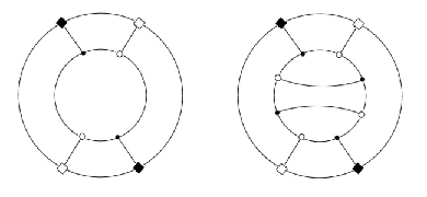
Refer to caption
Figure 16: Invariant differential operators O^0{\hat{O}}_{0} and O^2{\hat{O}}_{2} for the case 3|33|3, represented as diagrams of tensor contraction. Black 3-valent vertices represent tensor SS, white 3-valent vertices represent tensor ϵ\epsilon, black 3-valent rhombuses represent tensor ∂/∂S\partial/\partial S, white 3-valent rhombuses represent tensor ϵ∗\epsilon_{*}. These operators cannot be used to find J3|3J_{3|3}, because they do not give any non-trivial equation on it.

The action of O^4{\hat{O}}_{4} on invariants and their products is given by

O^4​(I4I6)=(−1409​I42−983​I4​I6){\hat{O}}_{4}\ \left(\begin{array}[]{ccc}\\ I_{4}\\ \\ I_{6}\\ \\ \end{array}\right)=\left(\begin{array}[]{ccc}\\ -\dfrac{140}{9}I_{4}^{2}\\ \\ -\dfrac{98}{3}I_{4}I_{6}\\ \\ \end{array}\right)
O^4​(I42I4​I6I4​I6I62)=(13​I62−4729​I43−7709​I42​I6−7709​I42​I62563​I44−3403​I62​I4){\hat{O}}_{4}\ \left(\begin{array}[]{ccc}\\ I_{4}^{2}&I_{4}I_{6}\\ \\ I_{4}I_{6}&I_{6}^{2}\\ \\ \end{array}\right)=\left(\begin{array}[]{ccc}\\ \dfrac{1}{3}I_{6}^{2}-\dfrac{472}{9}I_{4}^{3}&-\dfrac{770}{9}I_{4}^{2}I_{6}\\ \\ -\dfrac{770}{9}I_{4}^{2}I_{6}&\dfrac{256}{3}I_{4}^{4}-\dfrac{340}{3}I_{6}^{2}I_{4}\\ \\ \end{array}\right)

Applying (28), we obtain

O^4​F​(I4,I6)=−1409​I42​∂F∂I4−983​I4​I6​∂F∂I6+(16​I62−329​I43)​∂2F∂I42−1123​I42​I6​∂2F∂I4​∂I6+(1283​I44−24​I4​I62)​∂2F∂I62{\hat{O}}_{4}F\big(I_{4},I_{6}\big)=-\dfrac{140}{9}I_{4}^{2}\dfrac{\partial F}{\partial I_{4}}-\dfrac{98}{3}I_{4}I_{6}\dfrac{\partial F}{\partial I_{6}}+\left(\dfrac{1}{6}I_{6}^{2}-\dfrac{32}{9}I_{4}^{3}\right)\dfrac{\partial^{2}F}{\partial I_{4}^{2}}-\dfrac{112}{3}I_{4}^{2}I_{6}\dfrac{\partial^{2}F}{\partial I_{4}\partial I_{6}}+\left(\dfrac{128}{3}I_{4}^{4}-24I_{4}I_{6}^{2}\right)\dfrac{\partial^{2}F}{\partial I_{6}^{2}}

For the integral discriminant, this expression vanishes. Substituting the ansatz (33) and making the necessary algebraic transformations, we obtain a differential equation on the function G⁡(z)G(z):

(144​z2+1536​z)​∂2G⁡(z)∂z2+(216​z+768)​∂G⁡(z)∂z+5​G​(z)=0\displaystyle(144z^{2}+1536z)\dfrac{\partial^{2}G(z)}{\partial z^{2}}+\left(216z+768\right)\dfrac{\partial G(z)}{\partial z}+5G(z)=0 (34)

which is nothing but Gauss hypergeometric equation

t⁡(1−t)​∂2G⁡(t)∂t2+(c−(a+b+1)​t)​∂G⁡(t)∂t−a​b​G​(t)=0t(1-t)\dfrac{\partial^{2}G(t)}{\partial t^{2}}+\left(c-(a+b+1)t\right)\dfrac{\partial G(t)}{\partial t}-abG(t)=0

with a=1/12a=1/12, b=5/12b=5/12, c=1/2c=1/2 and t=−3/32zt=-3/32z. This is the invariant form of n=3,r=3n=3,r=3 Ward identities.

Solution.

In terms of the Gauss hypergeometric function, the integral discriminant equals

J3|3(S)=c1⋅I4−1/42F1([112,512],[12],−3​I6232​I43)+c2⋅I6I4−7/42F1([712,1112],[32],−3​I6232​I43)\boxed{\begin{gathered}\ \ \ J_{3|3}\big(S\big)=c_{1}\cdot I_{4}^{-1/4}{}_{2}F_{1}\left(\left[\dfrac{1}{12},\dfrac{5}{12}\right],\left[\dfrac{1}{2}\right],-\dfrac{3I_{6}^{2}}{32I_{4}^{3}}\right)+c_{2}\cdot I_{6}I_{4}^{-7/4}{}_{2}F_{1}\left(\left[\dfrac{7}{12},\dfrac{11}{12}\right],\left[\dfrac{3}{2}\right],-\dfrac{3I_{6}^{2}}{32I_{4}^{3}}\right)\ \ \ \end{gathered}} (35)

where c1,2c_{1,2} are the two constants, parametrising the general solution of Ward identities. Particular solutions

J3|3(1)(S)=I4−1/4F12([112,512],[12],−3​I6232​I43) and J3|3(2)(S)=I6I4−7/4F12([712,1112],[32],−3​I6232​I43)J^{(1)}_{3|3}\big(S\big)=I_{4}^{-1/4}{}_{2}F_{1}\left(\left[\dfrac{1}{12},\dfrac{5}{12}\right],\left[\dfrac{1}{2}\right],-\dfrac{3I_{6}^{2}}{32I_{4}^{3}}\right)\ \ \ \mbox{ and }\ \ \ J^{(2)}_{3|3}\big(S\big)=I_{6}I_{4}^{-7/4}{}_{2}F_{1}\left(\left[\dfrac{7}{12},\dfrac{11}{12}\right],\left[\dfrac{3}{2}\right],-\dfrac{3I_{6}^{2}}{32I_{4}^{3}}\right)

are associated with different integration contours and can be called the first and the second branches of J3|3J_{3|3}. One can see, that the results of this section are parallel to those of sec.3.2 – even the rational parameters in the hypergeometric function are the same.

Singularities.

Notice, that the point t=1t=1 corresponds to

−3​I6232​I43=1-\dfrac{3I_{6}^{2}}{32I_{4}^{3}}=1

which is just the discriminant’s vanishing locus 32​I43+3​I62=D3|3=032I_{4}^{3}+3I_{6}^{2}=D_{3|3}=0. To investigate the two other suspicious points t=0t=0 and t=∞t=\infty, let us study asymptotics at these points. Using (19), we find

J3|3(1)(S)∼I4−1/4+O(t), when t→0J^{(1)}_{3|3}\big(S\big)\sim I_{4}^{-1/4}+O\big(t\big),\ \ \ \ \mbox{ when }t\rightarrow 0
J3|3(2)(S)∼I6I4−7/4+O(t), when t→0J^{(2)}_{3|3}\big(S\big)\sim I_{6}I_{4}^{-7/4}+O\big(t\big),\ \ \ \ \mbox{ when }t\rightarrow 0

Using (20), we find

J3|3(1)(S)∼−Γ⁡(1/2)Γ⁡(1/12)​Γ​(5/12)I4−1/4log(1+3​I6232​I43)+O(t0), when t→1J^{(1)}_{3|3}\big(S\big)\sim\dfrac{-\Gamma(1/2)}{\Gamma(1/12)\Gamma(5/12)}I_{4}^{-1/4}\log\big(1+\dfrac{3I_{6}^{2}}{32I_{4}^{3}}\big)+O\big(t^{0}\big),\ \ \ \ \mbox{ when }t\rightarrow 1
J3|3(2)(S)∼−Γ⁡(3/2)Γ⁡(7/12)​Γ​(11/12)I6I4−7/4log(1+3​I6232​I43)+O(t0), when t→1J^{(2)}_{3|3}\big(S\big)\sim\dfrac{-\Gamma(3/2)}{\Gamma(7/12)\Gamma(11/12)}I_{6}I_{4}^{-7/4}\log\big(1+\dfrac{3I_{6}^{2}}{32I_{4}^{3}}\big)+O\big(t^{0}\big),\ \ \ \ \mbox{ when }t\rightarrow 1

Using (19) and (21), we find

J3|3(1)(S)∼Γ⁡(1/2)​Γ​(1/3)Γ​(5/12)2(332)−1/12I6−1/6+O(t−5/12), when t→∞J^{(1)}_{3|3}\big(S\big)\sim\dfrac{\Gamma(1/2)\Gamma(1/3)}{\Gamma(5/12)^{2}}\left(\dfrac{3}{32}\right)^{-1/12}I_{6}^{-1/6}+O\big(t^{-5/12}\big),\ \ \ \ \mbox{ when }t\rightarrow\infty
J3|3(2)(S)∼Γ⁡(1/3)​Γ​(3/2)Γ​(11/12)2(332)−7/12I6−1/6+O(t−11/12), when t→∞J^{(2)}_{3|3}\big(S\big)\sim\dfrac{\Gamma(1/3)\Gamma(3/2)}{\Gamma(11/12)^{2}}\left(\dfrac{3}{32}\right)^{-7/12}I_{6}^{-1/6}+O\big(t^{-11/12}\big),\ \ \ \ \mbox{ when }t\rightarrow\infty

We can see from these results, that singularities of the integral discriminant J3|3J_{3|3} at finite values of I4,I6I_{4},I_{6} are completely controlled by the algebraic discriminant D3|3D_{3|3}. The singularity at discriminant locus is logarithmic. Other singularities, not related to the algebraic discriminant, are situated at infinite values of invariants: I4→∞I_{4}\rightarrow\infty (t→0t\rightarrow 0) and I6→−∞I_{6}\rightarrow-\infty (t→∞t\rightarrow\infty).

Hypergeometric integral.

Using eq. (22) once again, we obtain

J3|3​(S)=c1⋅∫01d​s​s−7/12(1−s)−11/12(32​I43+3​s​I62)1/12+c2​I6⋅∫01d​s​s−1/12(1−s)−5/12(32​I43+3​s​I62)7/12\boxed{\begin{gathered}J_{3|3}\big(S\big)=c_{1}\cdot\int\limits_{0}^{1}ds\ \dfrac{s^{-7/12}(1-s)^{-11/12}}{(32I_{4}^{3}+3sI_{6}^{2})^{1/12}}+c_{2}I_{6}\cdot\int\limits_{0}^{1}ds\ \dfrac{s^{-1/12}(1-s)^{-5/12}}{(32I_{4}^{3}+3sI_{6}^{2})^{7/12}}\end{gathered}} (36)

Just as in the case of J2|4J_{2|4}, it is possible to make the transformation (25), which gives

J3|3(1)(S)=(D3|3)−1/12F12([112,112],[12],3​I6232​D3|3)J^{(1)}_{3|3}\big(S\big)=\left(D_{3|3}\right)^{-1/12}{}_{2}F_{1}\left(\left[\dfrac{1}{12},\dfrac{1}{12}\right],\left[\dfrac{1}{2}\right],\dfrac{3I_{6}^{2}}{32D_{3|3}}\right)
J3|3(2)(S)=I6(D3|3)−7/12F12([712,712],[32],3​I6232​D3|3)J^{(2)}_{3|3}\big(S\big)=I_{6}\left(D_{3|3}\right)^{-7/12}{}_{2}F_{1}\left(\left[\dfrac{7}{12},\dfrac{7}{12}\right],\left[\dfrac{3}{2}\right],\dfrac{3I_{6}^{2}}{32D_{3|3}}\right)

We conclude, that cases 2|42|4 and 3|33|3 literally correspond one to another. From the point of view of discriminant theory, this is a remarkable correspondence: discriminant D2|4D_{2|4} is a simple two-dimensional discriminant, which is well-known and studied, while D3|3D_{3|3} is a three-dimensional discriminant, much more complicated and less widely known. The study of integral discriminants reveals a parallel between these two cases.

4 Conclusion

In this paper we have described the first steps into the study of non-Gaussian averages

Jn|r​(S)=∫d​x1​…​d​xn​e−S⁡(x1,…,xn)= function of invariants of ​SJ_{n|r}\big(S\big)=\int dx_{1}\ldots dx_{n}\ e^{-S(x_{1},\ldots,x_{n})}=\mbox{ function of invariants of }S

which are functions only of S​L​(n)SL(n) invariants of SS, because of inherent S​L​(n)SL(n) symmetry. The real motivation of this study is generalisation of the well-known Gaussian formula

Jn|2​(S)=∫d​x1​…​d​xn​e−Si​j​xi​xj=1detSJ_{n|2}\big(S\big)=\int dx_{1}\ldots dx_{n}\ e^{-S_{ij}x_{i}x_{j}}=\dfrac{1}{\sqrt{\det S}}

to non-quadratic forms SS. If found, such generalisation may immediately have a wide range of applications in statistical physics and quantum field theory. We have worked out several low-dimensional cases and present the results in the form of the following table:

nr Invariants  Discriminant ​Dn|r Integral discriminant ​Jn|r22I2I2I2−1/223I4I2I4−1/624I2,I3I23−6​I32I2−1/4⋅∑i=0∞1i!⋅(1/12)i​(5/12)i(1/2)i⋅(6​I32I23)i25I4,I8,I12I42−64​I8I4−1/10⋅∑i,j=0∞1i!​j!⋅(3/10)i+j​(1/10)2​i+3​j​(1/10)j(2/5)i+2​j​(3/5)i+2​j⋅(16​I8I42)i(128​I123​I43)j32I3I3I3−1/233I4,I632​I43+3​I62I4−1/4⋅∑i=0∞1i!⋅(1/12)i​(5/12)i(1/2)i⋅(−3​I6232​I43)i……………\begin{array}[]{c|c|c|c|l}n&r&\mbox{ Invariants }&\mbox{ Discriminant }D_{n|r}&\mbox{ Integral discriminant }J_{n|r}\\ &&&\\ \hline\cr&&&\\ 2&2&I_{2}&I_{2}&\ I_{2}^{-1/2}\\ &&&\\ &&&\\ 2&3&I_{4}&I_{2}&\ I_{4}^{-1/6}\\ &&&\\ &&&\\ 2&4&I_{2},I_{3}&I_{2}^{3}-6I_{3}^{2}&\ I_{2}^{-1/4}\cdot\sum\limits_{i=0}^{\infty}\dfrac{1}{i!}\cdot\dfrac{(1/12)_{i}(5/12)_{i}}{(1/2)_{i}}\cdot\left(\dfrac{6I_{3}^{2}}{I_{2}^{3}}\right)^{i}\\ &&&\\ &&&\\ 2&5&I_{4},I_{8},I_{12}&I_{4}^{2}-64I_{8}&\ I_{4}^{-1/10}\cdot\sum\limits_{i,j=0}^{\infty}\dfrac{1}{i!j!}\cdot\dfrac{(3/10)_{i+j}(1/10)_{2i+3j}(1/10)_{j}}{(2/5)_{i+2j}(3/5)_{i+2j}}\cdot\left(\dfrac{16I_{8}}{I_{4}^{2}}\right)^{i}\left(\dfrac{128I_{12}}{3I_{4}^{3}}\right)^{j}\\ &&&\\ &&&\\ 3&2&I_{3}&I_{3}&\ I_{3}^{-1/2}\\ &&&\\ 3&3&I_{4},I_{6}&32I_{4}^{3}+3I_{6}^{2}&\ I_{4}^{-1/4}\cdot\sum\limits_{i=0}^{\infty}\dfrac{1}{i!}\cdot\dfrac{(1/12)_{i}(5/12)_{i}}{(1/2)_{i}}\cdot\left(-\dfrac{3I_{6}^{2}}{32I_{4}^{3}}\right)^{i}\\ &&&\\ &&&\\ \ldots&\ldots&\ldots&\ldots&\ldots\\ \end{array}

where

(a)k≡Γ⁡(a+k)Γ⁡(a)=a⁡(a+1)​⋯​(a+k−1)(a)_{k}\equiv\frac{\Gamma(a+k)}{\Gamma(a)}=a(a+1)\dotsb(a+k-1)

As one can see, these series posess a nice structure: they are all hypergeometric, i.e, their coefficients are ratios of Γ\Gamma-functions. Despite there are too few examples to make far-going conclusions, we conjecture that

Jn|r​(S)=∫d​x1​…​d​xn​e−S⁡(x1,…,xn)= hypergeometric function of invariants of ​SJ_{n|r}\big(S\big)=\int dx_{1}\ldots dx_{n}\ e^{-S(x_{1},\ldots,x_{n})}=\mbox{ hypergeometric function of invariants of }S

To support this conjecture, it is necessary at least to calculate a few more examples. As follows from the table Fig. 3, the next simplest examples would be J2|6J_{2|6}, J3|4J_{3|4} and J4|3J_{4|3}. Also, because of hypergeometric nature of integral discriminants, it is interesting to find their qq-deformation, as well as the CFT representations of these objects, in the spirit of [13]. Especially interesting is the interplay between non-trivial qq-deformation and action-independence of integral discriminants. Of course, most interesting would be generalization of our results to functional integrals, some independent attempts in this direction have already been made [14].

Acknowledgements

We are indebted to V.Dolotin and V.Tkachev for stimulating discussions. Our work is partly supported by Russian Federal Nuclear Energy Agency and the Russian President’s Grant of Support for the Scientific Schools NSh-3035.2008.2, by RFBR grant 07-02-00547, by the joint grants 09-01-92440-CE, 09-02-91005-ANF, 09-02-93105-CNRS and by the NWO project 047.011.2004.026. The work of Sh.Shakirov is also supported in part by the Moebius Contest Foundation for Young Scientists and by the Dynasty Foundation.

References

  • [1] V.Dolotin, QFT’s With Action of Degree 3 and Higher and Degeneracy of Tensors, hep-th/9706001
  • [2] V.Dolotin and A.Morozov, Introduction to Non-Linear Algebra, World Scientific, 2007, hep-th/0609022
  • [3] N. Beklemishev, Invariants of cubic forms of four variables, Moscow Univ.Bull. 37 (1982) 54-62;
    D. Hilbert, B. Sturmfels and R. Laubenbacher, Theory of algebraic invariants, Cambridge University Press (1993);
    H. Derksen and G. Kemper, Computational invariant theory. Invariant Theory and Algebraic Transformation Groups, Springer-Verlag, Berlin, encyclopaedia of Mathematical Sciences 130 (2002);
    B.Sturmfels, Algorithms in invariant theory, Springer-Verlag, New York (2008)
  • [4] I.M. Gelfand, M.M. Kapranov, and A.V. Zelevinsky, Discriminants, Resultants and Multidimensional Determinants, Birkhauser, 1994
  • [5] V.Dolotin, On discriminants of polylinear forms, arXiv:alg-geom/9511010; On invariant theory. alg-geom/9512011;
    Yu. Chernyakov and V. Dolotin, Operations and Identities in Tensor Algebra, arXiv:math/0501206
  • [6] D. Manocha and J.Canny, Multipolynomial Resultant Algorithms, J.Symb.Comp. 15 (1993) 99 – 122;
    C. Andrea, A.Dickenstein, Explicit formulas for the multivariate resultant, arXiv:math/0007036;
    D. Eisenbud and F.O. Schreyer, Resultants and Chow forms via exterior syzygies, J. Amer. Math. Soc. 16 (2003) 537-579, arXiv:math/0111040;
    V. Tapia, Polynomial identities for hypermatrices, math-ph/0208010; Invariant and polynomial identities for higher rank matrices, math-ph/0702001;
    Sh.Shakirov, Higher discriminants of polynomials, Theor.Math.Phys. 153(2) (2007) 1477, math/0609524;
    B. Gustafsson and V.Tkachev, The resultant on compact Riemann surfaces, arXiv:math/0710.2326, Comm. Math. Phys. 286 (2009) 313-358;
    A.Morozov and Sh.Shakirov, Analogue of the identity L​o​g​D​e​t=T​r​a​c​e​L​o​gLogDet=TraceLog for resultants, arXiv:0804.4632; Resultants and Contour Integrals, arXiv:0807.4539;
    A.Anokhina, A.Morozov and Sh.Shakirov, Resultant as Determinant of Koszul Complex, arXiv:0812.5013
  • [7] A.Gerasimov, A.Morozov and K.Selivanov, Bogolubov’s Recursion and Integrability of Effective Actions, Int.J.Mod.Phys. A16 (2001) 1531-1558, hep-th/0005053;
    A. Morozov and A. Niemi, Can Renormalization Group Flow End in a Big Mess? Nucl.Phys. B666 (2003) 311-336, arXiv:hep-th/0304178;
    V. Dolotin and A. Morozov, The Universal Mandelbrot Set. Beginning of the Story, arXiv:hep-th/0501235; Int.J.Mod.Phys. A23 (2008) 3613-3684, arXiv:hep-th/0701234;
    A. Morozov and M. Serbyn, Non-Linear Algebra and Bogolubov’s Recursion, Theor.Math.Phys. 154 (2008) 270-293, hep-th/0703258;
    An. Morozov, Universal Mandelbrot Set as a Model of Phase Transition Theory, JETP Lett. 86 (2007) 745-748, arXiv:nlin/0710.2315
  • [8] M. Penkava and L. Weldon, Infinity Algebras, Massey Products, and Deformations, math/9808058;
    B. Keller, Introduction to A-infinity algebras and modules, math/9910179;
    A. Tomasiello, A-infinity structure and superpotentials, hep-th/0107195;
    A.Losev, Lectures at Dombai and Dubna Schools, 2004;
    A.Kozak, Discretization of Chern-Simons-like Theories, 2004-2006, unpublished;
    P.Mnev, Notes on Symplicial BF Theory, hep-th/0610326; Discrete BF Theory, arXiv:0809.1160;
    V.Dolotin, A.Morozov and Sh.Shakirov, A∞A_{\infty}-structure on simplicial complexes, arXiv:0704.2609;
    Higher Nilpotent Analogues of A∞A_{\infty} Structure, Phys.Lett. B651 (2007) 71-73, arXiv:0704.2884
  • [9] I.M. Gelfand, M.M. Kapranov and A.V. Zelevinsky, Generalized Euler Integrals and AA- Hypergeometric Functions, Advances in Math. 84 (1990), 255-271;
    I.M. Gelfand, M.M. Kapranov and A.V. Zelevinsky, Hypergeometric Functions, Toric Varieties and Newton Polyhedra in Special Functions, M. Kashiwara, T. Miwa (eds.), ICM-90 Satellite Conference Proceedings, Springer-Verlag Tokyo, 1991;
    M. Passare and A. Tsikh, Algebraic Equations and Hypergeometric Series, in: The Legacy of Niels Henrik Abel, O. A. Laudal and R. Piene (eds.), Springer Verlag, Berlin, 2004;
    M. Passare, T. Sadykov and A. Tsikh, Singularities of Nonconfluent Hypergeometric Functions in Several Variables, arXiv:math/0405259;
    J. Stienstra, GKZ Hypergeometric Structures, math/0511351
  • [10] A.Morozov, Integrability and Matrix Models, Phys.Usp. 37 (1994) 1-55, hep-th/9303139; Matrix Models as Integrable Systems, hep-th/9502091;
    A.Alexandrov, A.Mironov and A.Morozov, Solving Virasoro Constraints in Matrix Models, Fortsch.Phys. 53 (2005) 512-521, hep-th/0412205;
    A.Mironov, Matrix Models vs. Matrix Integrals, Theor.Math.Phys. 146 (2006) 63-72, hep-th/0506158;
    S. Uhlmann, R. Meinel and A. Wipf, Ward Identities for Invariant Group Integrals, hep-th/0611170
  • [11] W.Lerche, D.Smit and N. Warner, Differential Equations for Periods and Flat Coordinates in Two Dimensionsional Topological Matter Theories, Nucl.Phys. B372 (1992) 87-112, hep-th/9108013;
    A. Ceresole, R. D’Auria, S. Ferrara, W. Lerche and J. Louis, Picard-Fuchs Equations and Special Geometry, Int.J.Mod.Phys. A8 (1993) 79-114, hep-th/9204035;
    A.Klemm, W.Lerche and S.Theisen, Nonperturbative Effective Actions of N=2N=2 Supersymmetric Gauge Theories, hep-th/9505150;
    M.Matone, Instantons and Recursion Relation in N=2N=2 Gauge Theory, hep-th/9506102; Koebe 1/4-Theorem and Inequalities in N=2N=2 Super-QCD, hep-th/9506181;
    S.Kachru, A.Klemm, W.Lerche, P.Mayr and C.Vafa, Nonperturbative Results on the Point-Particle Limit of N=2N=2 Heterotic String Compactification, hep-th/9508155;
    H. Itoyama and A. Morozov, Prepotential and the Seiberg-Witten Theory, Nucl.Phys. B491 (1997) 529-573, hep-th/9512161;
    M. Alishahiha, On the Picard-Fuchs equations of the SW models, Phys.Lett. B398 (1997) 100-103, hep-th/9609157;
    J. Isidro, Integrability, Seiberg-Witten Models and Picard-Fuchs Equations, JHEP 0101 (2001) 043, hep-th/0011253
  • [12] M. Abramowitz and I. Stegun, Handbook of Mathematical Functions with Formulas, Graphs, and Mathematical Tables, 9th printing. Dover, New York, (1972);
    I. Gradstein and I. Ryzhik, Tables of Integrals, Series and Products, New York: Academic (1980)
  • [13] A.Morozov and L.Vinet, qq–Hypergeometric Functions in the Formalism of Free Fields, Mod.Phys.Lett. A8 (1993) 2891-2902, arXiv:hep-th/9309026
  • [14] J. Bohacik and P. Presnajder, Functional integral with p​h​i4phi^{4} term in the action beyond standard perturbative methods, hep-th/0503235; Nonperturbative approach to(Wiener) functional integral with ϕ4\phi^{4} interaction, hep-th/0507129; Functional integral with ϕ4\phi^{4} term in the action beyond standard perturbative methods II, arXiv:0711.4683