Non-Fermi liquids from holography

The action for a vector field $A_{M}$ coupled to AdS₄ gravity can be written as

$$S={1\over 2\kappa^{2}}\int d^{4}x\,\sqrt{-g}\left[{{\mathcal{R}}}-{6\over R^{2}}-{R^{2}\over g_{F}^{2}}F_{MN}F^{MN}\right]$$

(2)

where $g_{F}^{2}$ is an effective dimensionless gauge coupling⁴⁴ 4 It is defined so that for a typical supergravity Lagrangian it is a constant of order $O(1)$. The equations of motion following from (2) are solved by the geometry of a charged black hole [19, 18]⁵⁵ 5 For a generic embedding of (2) into 4d ${\cal N}=2$ supergravity, this solution can be lifted to an M-theory solution [20].

$$ds^{2}={r^{2}\over R^{2}}(-fdt^{2}+dx_{i}^{2})+{R^{2}dr^{2}\over r^{2}f}$$

(3)

with

$$f=1+{Q^{2}\over r^{4}}-{M\over r^{3}},\quad A_{0}=\mu\left(1-{r_{0}\over r}\right),\quad\mu\equiv{g_{F}Q\over R^{2}r_{0}}$$

(4)

where $r_{0}$ is the horizon radius determined by $f(r_{0})=0$, and $\mu$ can be identified as the chemical potential of the boundary theory. For calculational purposes it is convenient to use dimensionless quantities. Consider the rescaling

	$\displaystyle r\to r_{0}r,\quad(t,\vec{x})\to{R^{2}\over r_{0}}(t,\vec{x}),\quad A_{0}\to{r_{0}\over R^{2}}A_{0},$
	$\displaystyle\qquad\quad M\to Mr_{0}^{3},\quad Q\to Qr_{0}^{2}$		(5)

after which the metric becomes

$${ds^{2}\over R^{2}}\equiv g_{MN}dx^{M}dx^{N}=r^{2}(-fdt^{2}+d\vec{x}^{2})+{1\over r^{2}}{dr^{2}\over f},\qquad$$

(6)

with now the horizon at $r=1$ and

$$f=1+{Q^{2}\over r^{4}}-{1+Q^{2}\over r^{3}},\quad A_{0}=\mu\left(1-{1\over r}\right),\quad\mu=g_{F}Q\ .$$

(7)

The dimensionless temperature is given by

$$T={1\over 4\pi}\left(3-Q^{2}\right)\ .$$

(8)

The zero-temperature limit is obtained by setting $Q=\sqrt{3}$. At zero temperature, near the horizon the metric (6) becomes $AdS_{2}\times{\mathbb{{R}}}^{2}$ with the curvature radius of $AdS_{2}$ given by

$$R_{2}={R\over\sqrt{6}}\ .$$

(9)

To compute the spectral functions for ${{\mathcal{O}}}$ we need only the quadratic action of $\psi$ in the geometry (6)-(9)

$$S_{\rm spinor}=\int d^{d+1}x\sqrt{-g}\,i(\bar{\psi}{{\Gamma}}^{M}{{\mathcal{D}}}_{M}\psi-m{\bar{\psi}}\psi)$$

(10)

where

$${\bar{\psi}}=\psi^{\dagger}{{\Gamma}}^{\underline{t}},\quad{{\mathcal{D}}}_{M}=\partial_{M}+{1\over 4}\omega_{abM}{{\Gamma}}^{ab}-iqA_{M}$$

(11)

and $\omega_{abM}$ is the spin connection⁶⁶ 6 We will use $M$ and $a,b$ to denote bulk spacetime and tangent space indices respectively, and $\mu,\nu\cdots$ to denote indices along the boundary directions, i.e. $M=(r,\mu)$. All indices on Gamma matrices refer to tangent space ones. For notational convenience below we will take $m$ to be defined in units of $1/R$, i.e. $mR\to m$.. Note that the Dirac action (10) depends on $q$ only through

$$\mu_{q}\equiv\mu q=g_{F}qQ$$

(12)

i.e. through the combination of $g_{F}q$. This is expected; $\mu$ is the minimal amount energy needed to add a unit charge to the system, thus for a field of charge $q$, the effective chemical potential is given by $\mu_{q}$. Below, for notational simplicity, we will set $g_{F}=1$ and treat $q$ as a free parameter, but one should keep in mind only the product of them is the relevant quantity.

To analyze the Dirac equations following from (10), it is convenient to use the following basis

$${{\Gamma}}^{r}=\left(\begin{array}[]{cc}1&0\\ 0&-1\end{array}\right),\;\;{{\Gamma}}^{\mu}=\left(\begin{array}[]{cc}0&{{\gamma}}^{\mu}\\ {{\gamma}}^{\mu}&0\end{array}\right),\;\;\psi=\left(\begin{array}[]{c}\psi_{+}\\ \psi_{-}\end{array}\right)$$

(13)

where $\psi_{\pm}$ are two-component spinors and ${{\gamma}}^{\mu}$ are gamma matrices of the (2+1)-dimensional boundary theory. Writing

$$\psi_{\pm}=(-gg^{rr})^{-{1\over 4}}e^{-i\omega t+ik_{i}x^{i}}\phi_{\pm}\ ,$$

(14)

the Dirac equation becomes

$$\sqrt{g_{ii}\over g_{rr}}\left(\partial_{r}\mp m\sqrt{g_{rr}}\right)\phi_{\pm}=\mp iK_{\mu}{{\gamma}}^{\mu}\phi_{\mp},$$

(15)

with

$$K_{\mu}(r)=\left(-u(r),k_{i}\right),\qquad u=\sqrt{g_{ii}\over-g_{tt}}(\omega+\mu_{q}(1-{1\over r}))\ .$$

(16)

Note that since as $r\to\infty$, $u\to\omega+\mu_{q}$, $\omega$ should correspond to the difference of the boundary theory frequency from $\mu_{q}$, i.e. $\omega=0$ corresponds to the Fermi energy.

To extract the retarded Green function for ${{\mathcal{O}}}$, we need to solve (15) with the in-falling boundary condition at the horizon [15], and to identify the source and the expectation value for ${{\mathcal{O}}}$ from the asymptotic behavior of $\psi$ near the boundary. Such an identification can be carried out from the prescription of [16, 17], which amounts to identifying $\psi_{+}$ as the source and its canonical momentum in terms of $r$-slicing (which is essentially $\psi_{-}$) as the expectation value. More explicitly, $\phi_{\pm}$ have the following asymptotic behavior near $r\to\infty$,

$$\phi_{+}=Ar^{m}+Br^{-m-1},\;\phi_{-}=Cr^{m-1}+Dr^{-m}\$$

(17)

with

$$C={i{{\gamma}}^{\mu}k_{\mu}\over 2m-1}A,\;B={i{{\gamma}}^{\mu}k_{\mu}\over 2m+1}D,\;k_{\mu}=(-(\omega+\mu_{q}),k_{i})\ .$$

(18)

Suppose the coefficients $D$ (corresponding to expectation value) and $A$ (corresponding to source) are related by $D={\mathcal{S}}A$, then the retarded Green function $G_{R}$ is given by [17]⁷⁷ 7 Here we assume $m\geq 0$. For $m<0$, one simply exchanges the roles of $A$ and $D$. For $m\in[0,{{\frac{1}{2}}})$, both quantization procedures are allowed. Also note that the factor ${{\gamma}}^{0}$ in (19) comes from $G_{R}\sim{\left\langle{\{{{\mathcal{O}}},{{\mathcal{O}}}^{\dagger}\}}\right\rangle}$ while in perturbing the boundary action we add $-i\int d^{3}x\,(\bar{\psi}_{0}{{\mathcal{O}}}+\bar{{\mathcal{O}}}\psi_{0})$ with $\bar{{\mathcal{O}}}={{\mathcal{O}}}^{\dagger}{{\gamma}}^{0}$. As noted in [17], we must choose the sign of the overall gravity action to be consistent with unitarity.

$$G_{R}=-i{\mathcal{S}}{{\gamma}}^{0}\ .$$

(19)

Equations (15) can be further simplified by choosing the basis ${{\gamma}}^{0}=i\sigma_{2},{{\gamma}}^{1}=\sigma_{1},\gamma^{2}=\sigma_{3}$ and setting $k_{2}=0$,⁸⁸ 8 Since the system is rotationally symmetric, there is no loss of generality. after which one finds two sets of decoupled equations

	$\displaystyle\sqrt{g_{ii}\over g_{rr}}\left(\partial_{r}\mp m\sqrt{g_{rr}}\right)y_{\pm}=\mp i(k_{1}-u)z_{\mp},$		(20)
	$\displaystyle\sqrt{g_{ii}\over g_{rr}}\left(\partial_{r}\pm m\sqrt{g_{rr}}\right)z_{\mp}=\pm i(k_{1}+u)y_{\pm}$		(21)

where we have written $\phi_{\pm}=\left(\begin{array}[]{c}y_{\pm}\\ z_{\pm}\end{array}\right)$. Introducing the ratios

$$\xi_{+}={iy_{-}\over z_{+}},\qquad\xi_{-}=-{iz_{-}\over y_{+}},$$

(22)

and using (19), the retarded Green function $G_{R}$ can be written as

$$G_{R}=\lim_{\epsilon\to 0}\epsilon^{-2m}\left(\begin{array}[]{cc}\xi_{+}&0\\ 0&\xi_{-}\end{array}\right)\biggr|_{r={1\over\epsilon}},$$

(23)

where one should extract the finite terms in the limit.

It is convenient to derive flow equations directly for $\xi_{\pm}$ as in [16]. From (20), we find

$$\sqrt{g_{ii}\over g_{rr}}\partial_{r}\xi_{\pm}=-2m\sqrt{g_{ii}}\xi_{\pm}\mp(k_{1}\mp u)\pm(k_{1}\pm u)\xi_{\pm}^{2}$$

(24)

The in-falling boundary condition at the horizon implies

$$\xi_{\pm}|_{r=1}=i\ .$$

(25)

With the boundary condition (25), one can now integrate (24) to $r\to\infty$ to obtain the boundary correlation function directly. Below we will drop the subscript $1$ on $k_{1}$.

At zero temperature, the $\omega\to 0$ limit of equations (20)–(21) and (24) is singular, since $g_{tt}$ then has a double zero at the horizon. As we will see this has important consequences for the behavior of $G_{R}$ near $\omega=0$. Also, at $\omega=0$ the in-falling boundary conditions (25) do not apply and should be replaced by

$$\xi_{\pm}|_{r=1,\,\omega=0}={m-\sqrt{k^{2}+m^{2}-{\mu_{q}^{2}\over 6}-i\epsilon}\over{\mu_{q}\over\sqrt{6}}\pm k}\ .$$

(26)

Note that the $1/\sqrt{6}$ factor multiplying $\mu_{q}$ in (26) has the same origin as the one appearing in (9).

We now describe the properties of $G_{R}$ obtained by solving (24). First note that by taking $k\to-k$ the equations for $\xi_{\pm}$ exchange with each other, leading to

$$G_{22}(\omega,k)=G_{11}(\omega,-k)\ .$$

(27)

Similarly by taking $q\to-q,\omega\to-\omega$ we find that

$$G_{11}(\omega,k;-q)=-G_{22}^{*}(-\omega,k;q)\ .$$

(28)

So it is enough to restrict to positive $k$ and $q$. One can also check that as $|\omega|,|k|\gg\mu_{q}$, both components reduce to those of the vacuum. When $m=0$, by dividing the equation for $\xi_{+}$ in (24) by $\xi_{+}^{2}$, we find that $\xi_{-}=-{1\over\xi_{+}}$, which implies that

$$G_{22}(\omega,k)=-{1\over G_{11}(\omega,k)},\qquad m=0\ .$$

(29)

Combining (27) and (29) we thus conclude that at $k=0$,

$$G_{11}(\omega,k=0)=G_{22}(\omega,k=0)=i,\quad m=0\ .$$

(30)

Further study of $G_{R}$ is possible by numerically solving (24). We will first consider $T=0$ and will mostly discuss the massless case. The mass dependence will be discussed briefly at the end. There are several consistency checks on our numerics. Firstly, $\textrm{Im}\,G_{11}$ and $\textrm{Im}\,G_{22}$ are both positive, which is a requirement of unitarity since the diagonal components are proportional to spectral densities. For a fixed large $k\gg\mu_{q}$, $\textrm{Im}\,G_{11}$ has a linearly-dispersing constant-height peak at $\omega+\mu_{q}\approx-k$ and $\textrm{Im}\,G_{22}$ has a peak at $\omega+\mu_{q}\approx k$, while both components are roughly zero in the region $\omega+\mu_{q}\in(-k,k)$ (see figure 1 and 2). This recovers the behavior in the vacuum, which is given by [21, 22]

$$G_{11}=-\sqrt{k-(\omega+i\epsilon)\over k+(\omega+i\epsilon)},\quad G_{22}=\sqrt{k+(\omega+i\epsilon)\over k-(\omega+i\epsilon)}$$

(31)

with now the divergences at $\omega=\pm k$ smoothed out into finite size peaks.

As one decreases $k$ to $\mu_{q}$ and smaller, the behavior of $G_{R}$ deviates significantly from that of the vacuum. For definiteness, let us now focus on $q=1$ (with $\mu_{q}=\sqrt{3}$). In this case the finite peak of $\textrm{Im}\,G_{22}$ in the large $k$ region develops into a sharp quasi-particle-like peak near $k_{F}=0.918528499(1)$ (see figure 2). The behavior of $\textrm{Im}\,G_{22}$ in the region of small $k_{\perp}\equiv k-k_{F}$ and $\omega$ can be summarized as follows:

1. 1.

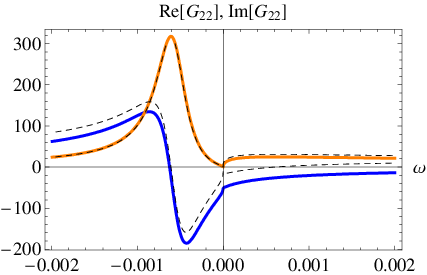
   For $k_{\perp}<0$, we find a sharp quasi-particle-like peak in the region $\omega<0$ and a small “bump” (with a broad maximum) in the region $\omega>0$ (see figure 3). This appears to indicate that there is a quasi-particle-like pole in the left quadrant of the lower-half complex $\omega$-plane. As $k_{\perp}\to 0_{-}$, both the peak and the maximum of the bump approach $\omega=0$, their heights go to infinity, and their widths go to zero. By carefully examining when the peak and the bump meet we are able to determine the accuracy of $k_{F}=0.918528499(1)$ to 10th digit.

2. 2.

   For $k_{\perp}>0$, one does not see a sharp peak along real $\omega$-axis for either sign of $\omega$. Instead one finds a “bump” (with a broad maximum) on the $\omega>0$ side and a smaller bump on the $\omega<0$ side. See figure 5. In the limit $k_{\perp}\to 0_{+}$, both bumps approach $\omega=0$ and their heights go into infinity.

3. 3.

   The quasi-particle-like peak and various bumps can also be studied by plotting $\textrm{Im}\,G_{22}(k,\omega)$ as a function of $k$ for a given $\omega$ (see the left panel of figure 4 for a plot at $\omega=-0.001$). In the limit $\omega\to 0_{-}$, the height of the peak goes to infinity with its width going to zero. At exactly $\omega=0$, however, the functions $\textrm{Im}\,G_{11}$ and $\textrm{Im}\,G_{22}$ become identically zero for $k>{\mu_{q}\over\sqrt{6}}={1\over\sqrt{2}}$ (see the right panel of figure 4). This behavior can be understood from (26) and (24) as follows. For $k\geq{\mu_{q}\over\sqrt{6}}$ (at $m=0$), the boundary conditions (26) become real and since (24) are real equations, $\textrm{Im}\,G_{ii}(\omega=0,k)$ are then identically zero in this region. Note that $k_{F}>{1\over\sqrt{2}}$.

Denoting the location of the maximum of the quasi-particle-like peak as $\omega_{*}(k_{\perp})$ we find that $\omega_{*}(k_{\perp})$ scales with $k_{\perp}\to 0_{-}$ as

$$\omega_{*}(k_{\perp})\sim k_{\perp}^{z},\qquad z=2.09\pm 0.01$$

(32)

and the height of $\textrm{Im}\,G_{22}$ at the maximum scales as

$$\textrm{Im}\,G_{22}(\omega_{*}(k_{\perp}),k_{\perp})\sim k_{\perp}^{-{\alpha}},\qquad{\alpha}=1.00\pm 0.01\$$

(33)

(see figure 6). One finds exactly the same scaling behavior also for the maxima of the other three “bumps”. This strongly suggests that in the limit of small $k_{\perp}$ and $\omega$ $\textrm{Im}\,G_{22}(\omega,k_{\perp})$ has the following scaling form

$$\textrm{Im}\,G_{22}(\lambda^{z}\omega,\lambda k_{\perp})=\lambda^{-{\alpha}}\textrm{Im}\,G_{22}(\omega,k_{\perp})$$

(34)

with the scaling exponents ${\alpha},z$ given by

$$z=2.09\pm 0.01,\qquad{\alpha}=1.00\pm 0.01\ .$$

(35)

The scaling behavior (32)–(35) suggests an underlying sharp Fermi surface with Fermi momentum $k_{F}$. It is, however, not of the form corresponding to a Landau Fermi liquid which would have exponents $z={\alpha}=1$. It is an example of the more general scaling behavior discussed recently by Senthil [23, 24] for a critical Fermi surface occurring at a continuous metal-insulator transition⁹⁹ 9 For early work, see [25, 26].. The system also has a rather curious particle-hole asymmetry; the quasi-particle-like peak at $k_{\perp}<0$ morphs into a “bump” at $k_{\perp}>0$ as the Fermi surface is crossed (compare feature 1 and 2 of previous page). The fact that $\mu_{q}>k_{F}$ suggests that the system has repulsive interactions.

For a given $\omega\neq 0$, $G_{ii}(k,\omega)$ are non-singular for any value of $k$ including $k_{F}$, while for a given value of $k$, $G_{ii}(k,\omega)$ is continuous but non-smooth at $\omega=0$.¹⁰¹⁰ 10 From numerical calculation, it does appear that the functions become smoother for $k\gg\mu_{q}$. This non-smooth behavior at $\omega=0$ for momenta away from the Fermi momentum is puzzling and it would be nice to understand its physical interpretation better. From the gravity side, this is related to the aforementioned singular behavior of equations (20)–(21) and (24) near $\omega\to 0$, as discussed around (26). This can be further attributed to the existence of an AdS₂ region (9) in the bulk geometry at zero temperature.

Further support for the scaling behavior (34) near the Fermi surface can be obtained by fitting the whole curves of $G_{22}(\omega)$ (rather than just the behavior near the maxima) for different $k_{\perp}$ by a scaling function which is analytic in the upper half $\omega$-plane¹¹¹¹ 11 We would like to thank S. Sachdev for a discussion of possible subtleties.:

1. 1.

   For $k_{\perp}<0$, $G_{22}$ can be fitted¹²¹² 12 The function fits well not only along the real $\omega$-axis, but also in the upper half plane. There are numerical instabilities at zero temperature in the lower half complex $\omega$-plane and we have not been able to perform a direct fit there. for both signs of $\omega$, by (see figure 3)

   $$G_{22}(\omega,k_{\perp})\approx{c_{0}(-k_{\perp})^{-{\alpha}}\over\log\left({-\omega\over c_{1}(-k_{\perp})^{z}}\right)-i{{\gamma}}}$$

   (36)

   where ${{\gamma}}\approx 0.34$ and $c_{0},c_{1}$ are positive constants (in the scaling region). The above function has a pole in the lower half $\omega$-plane at

   $$\omega_{c}=-c_{1}(-k_{\perp})^{z}e^{i{{\gamma}}}\ .$$

   (37)

   As $k_{\perp}\to 0_{-}$, $\omega_{c}$ approaches to the origin of the complex plane along a straight line which has an angle ${{\gamma}}-\pi$ with respect to the positive real axis. Since $\textrm{Re}\,\omega_{c}$ gives the location $\omega_{*}(k_{\perp})$ of the peak and $-\textrm{Im}\,\omega_{c}$ gives the width ${{\Gamma}}$ of the peak, for (36),

   $${{\Gamma}}=\tan{{\gamma}}\,|\omega_{*}(k_{\perp})|\ .$$

   (38)

   This linear dependence of the width on $\omega_{\star}$¹³¹³ 13 Recall that for a Landau quasi-particle, ${{\Gamma}}\sim\omega_{*}^{2}$. is reminiscent of the behavior in e.g. [2].

2. 2.

   For $k_{\perp}>0$, we have not found a good global fit for both signs of $\omega$. A reasonable fit for the imaginary part is

   $$G_{22}(\omega,k_{\perp})\approx{a_{0}k_{\perp}^{-{\alpha}}\over a_{1}-i\left({|\omega|\over k_{\perp}^{z}}\right)^{{\alpha}\over z}}~;$$

   (39)

   where $a_{0}$ and $a_{1}$ are positive constants which take different values for $\omega<0$ and $\omega>0$¹⁴¹⁴ 14 Again we are handicapped by a numerical instability the lower half $\omega$-plane which prevents a fit directly around the singularities in the lower half plane..

It is important to note that the functions (36) and (39) are only best numerical fits we could find and should not be taken too seriously as the “genuine” functions which describe the system. Both are consistent with the requirement from figure 4 that $\textrm{Im}\,G_{22}(k_{\perp})=0$ at $\omega=0$. The different fit functions for $k_{\perp}<0$ and $k_{\perp}>0$ may reflect the “particle-hole asymmetry” discussed earlier. Also note that for a nonzero $k_{\perp}$ both (36) and (39) indicate a branch point singularity at $\omega=0$, but have different $k_{\perp}\to 0$ limits. The behavior of $\textrm{Im}\,G_{22}(\omega)$ at exactly $k=k_{F}$ is not completely clear to us at the moment.

In the region $k<{\mu_{q}\over\sqrt{6}}$, where $\textrm{Im}\,G_{ii}(\omega=0,k)$ are nonzero (see figure 4), a new phenomenon occurs in the $\omega\to 0$ limit. One finds that $\textrm{Im}\,G_{ii}(\omega,k)$ become oscillatory with oscillatory peaks periodic in $\log|\omega|$ with constant heights, see fig. 7. More explicitly we find

$$G_{ii}(\omega,k)=G_{ii}(\omega e^{n\xi(k)},k),\qquad n\in{\mathbb{{Z}}},\quad\omega\to 0$$

(40)

where $\xi(k)$ is a ($k$-dependent) positive constant. In other words, $G_{ii}$ is invariant under a discrete scaling in $\omega$. $\xi(k)$ appears to decrease with $k$ and approaches a constant in the limit $k\to 0$. In the limit $k\to{\mu_{q}\over\sqrt{6}}$, $\xi(k)$ approaches infinity. The height of the oscillatory peaks also decreases with $k$, approaching zero as $k\to 0$ (where the whole function approaches unity) and a finite constant as $k\to{\mu_{q}\over\sqrt{6}}$. It would be interesting to understand whether (40) is associated with some kind of complex scaling exponents. Below we will refer to the region $k<{\mu_{q}\over\sqrt{6}}$ as the oscillatory region. Note that the oscillatory region appears to be the counterpart for fermions of the unstable region for a charged boson, where the corresponding bosonic modes have complex energies and want to condense. In the fermion case, the oscillatory region does not appear to indicate an instability, e.g. there is no singularity in the upper half of the complex $\omega$-plane.

Turning on a small temperature $T$ appears to smooth everything out. There is no longer a sharp Fermi surface, i.e. there no longer exists a sharp momentum at which $\textrm{Im}\,G_{22}$ becomes singular for any real $\omega$ and $k$. Going to the lower half $\omega$-plane, one finds that all the singularities are a finite distance away from the real axis, with the closest distance given by $T$ which happens at $k\approx 0.90$ (see figure 8)¹⁵¹⁵ 15 Similar results have also been obtained by Carlos Fuertes. We thank Carlos Fuertes and Subir Sachdev for communicating the results to us.. This behavior is different from the Fermi liquid where the width is quadratic in temperature. Note that for a given small $k_{\perp}<0$, as one turns on the temperature, the corresponding quasi-particle-like pole in the complex $\omega$-plane appears to move down and to the right. It is also interesting to note that at finite $T$, there are now quasi-particle-like poles for momenta $k>k_{F}$. Perhaps they are generated from the branch point at $T=0$.

At finite $T$, the functions $\textrm{Im}\,G_{ii}$ become smooth at $\omega=0$ and in the oscillatory region there are only a finite number of oscillations as the $\omega\to 0$ limit is approached.

When we increase (decrease) $q$ to be greater (smaller) than $1$, the Fermi momentum $k_{F}$ increases (decreases) with $q$ approximately linearly. As $q$ is further increased, new branches of Fermi surfaces appear. These features can be seen in figure 9, which gives the density plots of $\textrm{Im}\,G_{11}$ and $\textrm{Im}\,G_{22}$ in the $q-k$ plane at a fixed value of $\omega=-0.001$.

We have sampled the exponents $z,\alpha$ for a few other values of $q$ for the lowest branch of fermi surface in $\textrm{Im}\,G_{22}$, e.g. for $q=0.6$, $z\approx 5.32,\;\alpha\approx 1.00$, and for $q=1.2$, $z\approx 1.53,\;{\alpha}\approx 1.00$. Compared to the values for $q=1$ described earlier, it then appears that $z$ decreases rapidly with increasing $q$, while ${\alpha}=1$ is independent of $q$. Note that in [23] it was argued that $z\geq{\alpha}$ and $z\geq 1$. Thus it could be that $z$ will asymptote to $1$ for larger values of $q$.¹⁶¹⁶ 16 At larger values of $q$ the convergence of the exponents becomes slower; we leave this for future work. Also note that the value ${\alpha}=1$ is special according to the scaling theory of [23]. We also find that the constant ${{\gamma}}$ in (36) appears to decrease rapidly with $q$. Thus it seems likely that as $q$ is increased, the non-Fermi liquid will become more like a Landau Fermi liquid. Given that $k_{F}$ increases with $q$, this is reminiscent of asymptotic freedom in high-density QCD.

The $q-k$ space in figure 9 is separated into two regions by the (black) $k={\mu_{q}\over\sqrt{6}}$ line. In the region to right (stable region), the locations of the quasi-particle lines (i.e. orange lines in figure 9) stabilize in the limit $\omega\rightarrow 0$ and indicate locations of Fermi surfaces. The region to the left is the oscillatory region discussed earlier, where the log-periodic oscillatory behavior is reflected in a downward motion of the orange lines as $|\omega|$ is decreased; they seem to become infinitely dense in the limit $\omega\rightarrow 0$. Also recall that in the oscillatory region, the heights of the peaks remain finite in the $\omega\to 0$ limit.

As one decreases $q$, a Fermi surface line in figure 9 will intersect the line $k={\mu_{q}\over\sqrt{6}}$, disappear into the oscillatory region, and lose its status as a Fermi surface. Thus the behavior of $\textrm{Im}\,G_{ii}$ in the oscillatory region is strongly correlated with the sprouting of new branches of Fermi surface as $q$ is varied (see figure 10).

We have also studied other values of the mass (with $m<{\frac{1}{2}}$) at $q=1$, and find the Fermi momentum $k_{F}$ decreases linearly with increasing mass. At finite mass, the oscillatory region is now given by $k^{2}+m^{2}<{\mu_{q}^{2}\over 6}$ (see (26)). We find that for $q=1$, the Fermi surface disappears into the oscillatory region at roughly $m\approx 0.4$. For $m>{\mu_{q}\over\sqrt{6}}$, the oscillatory region disappears; we expect the Fermi surface will also disappear beyond this value if not before.

To conclude this section, let us summarize the main features of the spectral functions which we have observed. The system we study is conformally invariant at zero density. Turning on a finite charge density breaks Lorentz and scale invariance. The energy scale of the problem is controlled by the chemical potential $\mu$ which for a charge $q$ particle becomes $\mu_{q}=\mu q$. At $q=1$ the spectral functions also exhibit two other interesting scales. The first is the Fermi momentum $k_{F}<\mu_{q}$ around which we observe a quasi-particle-like peak which suggests an underlying Fermi surface. The scaling behavior and the particle-hole asymmetry around the Fermi surface indicate that this is a non-Fermi liquid. The other scale is $k_{S}\equiv{\mu_{q}\over\sqrt{6}}$, which lies below $k_{F}$. We find that for $k<k_{S}$, the spectral functions have log-periodic oscillatory behavior near $\omega=0$, which indicates some underlying discrete scale invariance. At larger values of $q$ new scales corresponding to more than branches of Fermi surface also appear.

It is important to emphasize that the scaling behavior observed here is not related to the scale invariance of the vacuum, which is broken by the nonzero charge density. It is emergent, arising as a consequence of the collective behavior of many particles. Note that both the scaling behavior around the Fermi surface and the discrete scale invariance involve the small $\omega$ limit, which on the gravity side can be attributed to the AdS₂ region in the near horizon geometry of the black hole at zero temperature. It may be possible that this emergent scaling behavior can be understood from the AdS₂ region¹⁷¹⁷ 17 Work in progress with T. Faulkner [27]..

References

- [1] P. W. Anderson, Phys. Rev. Lett. 64, 1839 (1990).
- [2] C. M. Varma, P. B. Littlewood, S. Schmitt-Rink, E. Abrahams, and A. E. Ruckenstein, Phys. Rev. Lett. 63, 1996 (1989).
- [3] C. M. Varma, Z. Nussinov, and W. van Saarloos, Physics Reports 361, 267 (2002), eprint cond-mat/0103393.
- [4] G. Benfatto and G. Gallavotti, Journal of Statistical Physics 59, 541 (1990).
- [5] R. Shankar, Physica A177, 530 (1991).
- [6] J. Polchinski (1992), eprint hep-th/9210046.
- [7] R. Shankar, Rev. Mod. Phys. 66, 129 (1994).
- [8] J. M. Maldacena, Adv. Theor. Math. Phys. 2, 231 (1998), eprint hep-th/9711200.
- [9] S. S. Gubser, I. R. Klebanov, and A. M. Polyakov, Phys. Lett. B428, 105 (1998), eprint hep-th/9802109.
- [10] E. Witten, Adv. Theor. Math. Phys. 2, 505 (1998), eprint hep-th/9803131.
- [11] J. Bagger and N. Lambert, JHEP 02, 105 (2008), eprint 0712.3738.
- [12] A. Gustavsson, Nucl. Phys. B811, 66 (2009), eprint 0709.1260.
- [13] O. Aharony, O. Bergman, D. L. Jafferis, and J. Maldacena, JHEP 10, 091 (2008), eprint 0806.1218.
- [14] S.-S. Lee (2008), eprint 0809.3402.
- [15] D. T. Son and A. O. Starinets, JHEP 09, 042 (2002), eprint hep-th/0205051.
- [16] N. Iqbal and H. Liu, Phys. Rev. D79, 025023 (2009a), eprint 0809.3808.
- [17] N. Iqbal and H. Liu (2009b), eprint 0903.2596.
- [18] A. Chamblin, R. Emparan, C. V. Johnson, and R. C. Myers, Phys. Rev. D60, 064018 (1999), eprint hep-th/9902170.
- [19] L. J. Romans, Nucl. Phys. B383, 395 (1992), eprint hep-th/9203018.
- [20] J. P. Gauntlett and O. Varela, Phys. Rev. D76, 126007 (2007), eprint 0707.2315.
- [21] M. Henningson and K. Sfetsos, Phys. Lett. B431, 63 (1998), eprint hep-th/9803251.
- [22] W. Mueck and K. S. Viswanathan, Phys. Rev. D58, 106006 (1998), eprint hep-th/9805145.
- [23] T. Senthil (2008a), eprint 0803.4009.
- [24] T. Senthil (2008b), eprint 0804.1555.
- [25] L. Yin and S. Chakravarty, Int. J. Mod. Phys. B10, 805 (1996).
- [26] S. Chakravarty, L. Yin, and E. Abrahams, Phys. Rev. B 58, R559 (1998).
- [27] T. Faulkner, H. Liu, J. McGreevy, and D. Vegh (2009), eprint 0907.2694.
- [28] S. S. Gubser, Phys. Rev. D78, 065034 (2008), eprint 0801.2977.
- [29] S. A. Hartnoll, C. P. Herzog, and G. T. Horowitz, Phys. Rev. Lett. 101, 031601 (2008), eprint 0803.3295.
- [30] F. Denef and S. A. Hartnoll (2009), eprint 0901.1160.
- [31] T. Holstein, R. E. Norton, and P. Pincus, Phys. Rev. B8, 2649 (1973).
- [32] M. Y. Reizer, Phys. Rev. B 40, 11571 (1989).
- [33] J. Polchinski, Nucl. Phys. B422, 617 (1994).
- [34] B. I. Halperin, P. A. Lee, and N. Read, Phys. Rev. B47, 7312 (1993).
- [35] C. Nayak and F. Wilczek, Nucl. Phys. B417, 359 (1994a), eprint cond-mat/9312086.
- [36] C. Nayak and F. Wilczek, Nucl. Phys. B430, 534 (1994b).
- [37] B. L. Altshuler, L. B. Ioffe, and A. J. Millis (1994), eprint cond-mat/9406024.
- [38] D. Boyanovsky and H. J. de Vega, Phys. Rev. D63, 034016 (2001), eprint hep-ph/0009172.
- [39] A. Ipp, A. Gerhold, and A. Rebhan, Phys. Rev. D69, 011901 (2004), eprint hep-ph/0309019.
- [40] T. Schafer and K. Schwenzer, Phys. Rev. D70, 054007 (2004), eprint hep-ph/0405053.