Excited-State Effective Masses in Lattice QCD
Abstract
We apply black-box methods, i.e. where the performance of the method does not depend upon initial guesses, to extract excited-state energies from Euclidean-time hadron correlation functions. In particular, we extend the widely used effective-mass method to incorporate multiple correlation functions and produce effective mass estimates for multiple excited states. In general, these excited-state effective masses will be determined by finding the roots of some polynomial. We demonstrate the method using sample lattice data to determine excited-state energies of the nucleon and compare the results to other energy-level finding techniques.
pacs
11.15.Ha,12.38.Gc,14.20.-c,02.60.-x,05.45.TpI Introduction
Lattice quantum chromodynamics (LQCD) has been used successfully to compute many experimentally observable quantities from first-principles calculation of Euclidean-time hadron correlation functions, even occasionally predicting experimental results before they are measured. However, the successes of LQCD have mostly been restricted to computation of the physical properties of the lowest-energy states in each quantum number channel by focusing on the large-time behavior of correlation functions where uncertainties due to excited-state contributions are exponentially suppressed. Given that signal-to-noise in correlation functions also falls exponentially at large times, success is often dictated by available computational resources.
Both in meson and baryon spectroscopy there are many experimentally observed excited states whose physical properties are poorly understood that could use theoretical input from LQCD to solidify their identification. Other excited-state quantities that could be computed on the lattice, such as form factors and coupling constants, would be useful to groups such as the Excited Baryon Analysis Center (EBAC) at Jefferson Lab, where dynamical reaction models have been developed to interpret experimentally observed properties of excited nucleons in terms of QCD [1, 2]. In certain cases, input from the lattice may be helpful in determining the composition of controversial states, which may be interpreted as ordinary hadrons, tetra- or pentaquarks, hadronic molecules or unbound resonances.
Among the excited nucleon states, the nature of the Roper resonance, , has been the subject of interest since its discovery in the 1960’s. It is quite surprising that the rest energy of the first excited state of the nucleon is less than the ground-state energy of nucleon’s negative-parity partner, the [3], a phenomenon never observed in meson systems. There are several interpretations of the Roper state, for example, as the hybrid state that couples predominantly to QCD currents with some gluonic contribution [4] or as a five-quark (meson-baryon) state [5].
Early LQCD calculations using the quenched approximation [6, 7, 8, 9, 10, 11, 12], found the computed spectrum inverted relative to experiment, with heavier than the . A recent study [7] suggested that qualitative agreement between experiment and LQCD in the quenched approximation could be restored provided other simulation effects due to finite volumes and unphysically heavy quarks were properly addressed. The study strongly suggests the nature of the Roper resonance changes dramatically as the quarks are made physically light in LQCD simulations, as in Fig. 1. Clearly, future LQCD calculations will require improved analysis techniques for extracting multiple excited-state energies, as well as variational wavefunctions, in the nucleon sector to test the validity of this claim.
| Group | (GeV) | (GeV) | (fm) | Method | Extrapolation | ||
|---|---|---|---|---|---|---|---|
| Basak et al. [13] | 0 | Wilson | 6.05 | 0.49 | 2.35 | VM | N/A |
| Burch et al. [12] | 0 | CIDO | 1.68,1.35 | 0.35–1.1 | 2.4 | VM | |
| Sasaki et al. [10] | 0 | Wilson | 2.1 | 0.61–1.22 | 1.5,3.0 | MEM | |
| Guadagnoli et al. [8] | 0 | Clover [14] | 2.55 | 0.51–1.08 | 1.85 | SBBM | |
| Leinweber et al. [9] | 0 | FLIC | 1.6 | 0.50–0.91 | 2.0 | VM | N/A |
| Mathur et al. [7] | 0 | Overlap [15] | 1.0 | 0.18–0.87 | 2.4,3.2 | CCF | |
| Sasaki et al. [6] | 0 | DWF | 2.1 | 0.56–1.43 | 1.5 | VM |

Apart from the vast amount of detail about excited states accessible to LQCD computations with advanced analysis methods, the statistical accuracy of ground-state quantities is also enhanced because correlation functions computed at shorter Euclidean times can be used where the signal-to-noise is greater. As current lattice simulations are performed with ever-greater resolution at short Euclidean times as lattice spacings are decreased toward the continuum limit, simultaneous extraction of ground and excited-state quantities will be essential to extract full value from such large-scale (and expensive) computations.
A variety of analysis techniques have been applied to extracting the excited-state spectrum from correlation functions. The most widely used method is a nonlinear least-squares (NLLS) fit to a model function, such as a sum over two or more exponentials. Operationally, even such a simple nonlinear fit can be fraught with difficulty, from establishing the range of Euclidean times included in the dataset to stabilizing the convergence of minimization algorithms by careful choices of initial guesses or temporarily freezing selected fit parameters during the minimization process, all of which require intervention by a trained expert.
At such times, the expert typically turns to black-box methods for guidance because they do not require intervention to determine initial guesses and fitting ranges: estimates of correlation functions go into the black box and estimates of hadron energies come out. The main detraction of black-box methods are that the produced estimates are expected to have larger uncertainties, making them sub-optimal relative to least squares methods [29]. Marrying the two approaches can effectively combine the best features of both, leading to a highly-automated analysis program producing optimal estimates of energies. Prior to this work, black-box methods were mainly useful for extracting ground-state and, perhaps, first excited-state energies [28, 8]. We believe the method described below will provide the needed black-box method for estimating as many energies from fixed set of correlations functions as are likely to be extracted from a NLLS fit.
The structure of this paper is as follows: Sec. II provides theoretical formulations of the excited-state effective masses for single and multiple correlators; it also explores certain extensions to these techniques: linear prediction and periodic boundary conditions. In Sec. III, we apply the methodology to some characteristic lattice correlators and compare the results with simple fitting and the variational method [23, 24]. Conclusions and future outlook are given in Sec. IV. Numerous details and examples are included in the appendices. Preliminary details of this work were presented in Ref. [30].
II Theoretical Basis
The hadron spectrum can be calculated in LQCD using two-point hadronic correlation functions
| (1) |
where the creation and annihilation operators and transform irreducibly under the symmetries of the lattice space group [31, 32, 33, 34]. After taking momentum (and spin for baryons) projection and inserting a complete set of hadronic eigenstates of the Hamiltonian (ignoring the variety of boundary condition choices possible), this becomes
| (2) |
where contains not only the overlap factor between the eigenstate and states created by the operators but also any kinetic factors that do not depend on Euclidean time separation .
II.1 Effective Masses
In general, a two-point correlation function computed on time-slices will admit an exact algebraic solution having the form of Eq. (2) with energies and amplitudes . The problem to solve is the nonlinear system of equations
| (3) |
for and where . is known as rectangular Vandermonde matrix.
By inspection, it appears the problem is of polynomial degree and thus by the Abel-Ruffini theorem [35, 36] should not admit a general closed form solution in terms of radicals for . The solution is simple to compute and is widely known in the lattice QCD literature as the effective mass solution. Note already that the simple effective mass problem is linear and has only one solution, suggesting that the polynomial degree is actually of order .
The solution was explicitly constructed by one of the authors [28] and was independently constructed some time later by others [8]. It was noted [28] that the problem, when reduced, required only the solution of a quadratic equation and so it was conjectured that the general problem of size could be reduced to a polynomial equation in one variable of degree .
An efficient algorithm has been available for some time for solving square Vandermonde systems [37] by making them upper triangular. This approach works equally well for rectangular Vandermonde systems as in Eq. (3). Furthermore, this approach reveals why the solution for the energies can be found without solving for the amplitudes and why the problem is of polynomial degree .
As a first step toward extracting the energies from our data, we transform the system so that is in upper triangular form [37] by pre-multiplying by the lower bi-diagonal matrices:
| (4) |
where the first on the diagonal appears in the row and column. In the appendices, we demonstrate in detail how the general solutions for , 3 and 4 work.
Finding a general approach for would be a tough challenge. Although Abel’s Impossibility Theorem proves there are no general solutions in radicals for polynomials higher than quartic order, there are numerical methods for finding the roots of polynomials of any order. The general form for the polynomial follows from Eqs. (), (45) and (87) in the appendices:
| (5) |
Prony [38] showed that problems in the form of Eq. (2) implied the following system of equations
| (6) |
where the matrix has the special structure of a Hankel matrix and the components of are the coefficients of a polynomial
| (7) |
The Prony-Yule-Walker method (or just Prony’s method, for short) [38, 39, 40] solves Eq. (6) to find the coefficients and then finds the roots of the polynomial in Eq. (7). The amplitudes are determined by substituting the roots into Eq. (3) and solving it. Note again that using timeslices of correlation function data to determine effective masses is a problem of polynomial order .
The general conditions under which the solutions of the Hankel and Vandermonde systems coincide is presented in Ref. [41]. Here we provide a simple demonstration that both solutions are the same under the assumption that there are no complications like degeneracies in the energy spectrum of Eq. (2). Assuming is invertible, solving Eq. (6) gives
| (8) |
for the polynomial of Eq. (7) and where . Recall that the inverse can be written in terms of the adjoint, or matrix of cofactors, , , where the notation means removing row and column . For Prony’s method, we can rescale and still find the roots by solving
| (9) |
for .
Returning to the Vandermonde method, the determinant of Eq. (5) can be expanded in terms of its cofactors
| (10) |
As usual, each cofactor can be expanded in terms of further cofactors where additional rows and columns are removed:
| (11) |
By eliminating the first row and last row of in Eq. (5) we recover and for the cofactors
| (12) |
so the desired identity is recovered
| (13) |
up to a possible overall minus sign for odd , which is irrelevant for finding roots. There is a unique set of solutions to the Vandermonde and Hankel systems (under the assumption of noise-free correlation functions with non-degenerate energy levels), so other considerations should determine which is the better method to construct the polynomial. It is our experience that computing coefficients from Eq. (5) is preferred to solving Eq. (6) as statistical noise in the correlation functions can lead to nearly singular Hankel matrices which are difficult to invert.
In an earlier work [28], one of the authors showed that Prony’s method (also called linear prediction) could easily be extended to use more than timeslices of a correlation function to extract only masses by constructing an over-constrained system of equations analogous to Eq. (6). It is not obvious how to construct and solve a similar over-constrained system in the Vandermonde case. Thus, Prony’s method has a potential advantage that more time samples of the correlation function can be used to extract the same number of energy levels leading to reduced statistical fluctuations.
II.2 Solutions with multiple correlation functions
When constructing correlation functions in LQCD, care is taken to ensure that the correlation function transforms irreducibly under the symmetries of the lattice space group [31, 32, 33, 34]. For the model function, as in Eq. (2), this implies that the amplitudes depend on the details of the specific correlation function but that the energies depend only on the irreducible representation. Since it is common in lattice QCD simulations to compute at least two distinct correlation functions for each irreducible representation, effective mass solutions which combine data from multiple correlations are also possible.
Assume that there are correlation functions available as in Eq. (2) that differ only in their amplitudes:
| (14) |
Data from the same time slices will be used in the following from each correlation function to construct effective masses. Under this assumption the condition that there will be equal number of data points as unknowns is . In Appendix A are the three solutions that satisfy the condition for , up to quartic order. There are four more solutions (up to quartic order) for : , , and (demonstrated in Appendix B). Relaxing the assumption that the same number of time slices are used from each correlation function will allow for more possibilities up to quartic order. It is straightforward to generalize to these cases if desired.
The general form of the polynomial equation can be inferred by studying the solved examples in Eqs. (), (116), (123) and (129). Define Hankel matrices for each of the correlation functions with the constraints and . Then the general form of the polynomial equation is
| (15) |
As previously discussed, each Hankel matrix is generally of full column rank and, if the correlation functions are linearly independent, then the columns of different Hankel matrices are also linearly independent. So, Eq. (15) will only be satisfied for discrete values of corresponding to the roots of the polynomial.
II.3 Periodic Boundary Conditions
In practical LQCD calculations, the temporal extent is finite so the choice of temporal boundary conditions affects hadronic correlation functions near the boundary. For simplicity, starting from Eq. (2), set and identify the points and which can be done using modular arithmetic, i.e. . For anti-periodic boundary conditions, the typical hadronic Euclidean time correlation function is described by the model function
| (16) |
For periodic boundary conditions, set . For mesons, but more importantly and , which is not true for baryons (). So, baryon correlation functions represent states propagating to the left and different states propagating to the right for a total of states.
Meson correlation functions represent the same states propagating to the right and left. However, time-reversal symmetry requires , up to noise terms, so that only half of the computed timeslices are truly independent. Thus, as was the case with baryons, information about only states in any given quantum number channel can be extracted from a single correlation function computed on timeslices in a finite box. As shown in Ref. [28], this can be made explicit by writing the meson correlation function as
| (17) |
To write this result in the Vandermonde form of Eq. (3), define the variables
| (18) |
When solving Eq. (3), the domain of the solutions will be the real numbers or complex conjugate pairs since real-valued correlation functions are used as input. Complex-valued solutions are clearly unphysical and should be discarded as they are likely due to noise. Real solutions may also be unphysical if they cannot be used to extract a non-negative energy, and this will depend on the details of the model function and hence the boundary conditions. For example, for the basic model of Eq. (2), only the solutions will yield non-negative energies. For mesons in periodic boxes, so only will yield non-negative energies. Finally, for baryons in periodic boxes, the states propagating to the right have and the states propagating to the left have so all solutions are physical and means the state is propagating to the left.
For some lattice fermion actions, e.g. staggered [42, 43, 44] or domain-wall fermions [45, 46], a variation of Eq. (2) is needed as a starting point to account for states which oscillate in time. For example, an appropriate model for staggered mesons on an infinite lattice is
| (19) |
There are two independently ordered sets of states, half of which oscillate as . When solving Eq. (3), such oscillating solutions will have physical solutions if . Similarly, for staggered baryons with periodic boundary conditions, physical solutions with are certainly expected as oscillating states moving to the left.
Generally speaking, model functions appropriate for the common lattice discretizations and choice of boundary conditions can be formulated and rewritten in the Vandermonde form of Eq. (3). The physical interpretation of the solutions depends on the details of the discretization and boundary conditions. In some cases, all real solutions may have a physical interpretation and thus cannot be immediately discarded without further statistical analysis.
III Numerical Results
Although the ground-state effective mass has a long tradition of use in the lattice QCD community, not much work has examined excited states and fewer yet their effective masses. In this section, we will demonstrate the application of these effective-mass techniques to some typical lattice correlation functions. At the end, we compare the results with the ones from variational method.
The data on which we demonstrate these methods is from a study done using the quenched approximation to QCD, i.e. where the effects of quantum fluctuations of quark-antiquark pairs in the vacuum are ignored, greatly reducing the computational cost but leading to an unknown, but hopefully small, systematic error. We generated an ensemble of anisotropic lattices with Wilson gauge action and nonperturbative clover fermion action using Dirichlet boundary condition. The spatial lattice spacing is about 0.125 fm with anisotropy 3 (that is, temporal spacing GeV). The parameters used in the fermion action give a 720-MeV pion. Specifically, our data are proton correlators using 7 Gaussian smearing parameters, 0.5–6.5 in steps of 1.0, including both smeared-point and smeared-smeared source-sink combinations. Fig. 2 shows the single-state effective-mass plots for these smeared-point proton correlators.

III.1 Excited-Effective Masses
We now apply the excited-effective masses to our nucleon data. In Fig. 3 we show the results of applying the single-correlator () excited-effective masses to the nucleon data for all with analytic solutions in terms of radicals. Notice that as the number of states included increases, the amount of early-time contamination is decreased. As the formulae better account for the exact form of the correlator, more of the time range can be reasonably used to determine the states. However, as the number of roots increases, the occurrence of “bad” roots (those that are negative or imaginary) tends to increase as well. Since these have to be thrown out, this causes gaps in the extracted states where the results are unreliable.

In Fig. 4 we show the results of applying the multiple correlator excited-effective masses to the nucleon data for all combinations of and that have solutions in terms of radicals. Notice that as the number of correlators increases, the quality of the extracted masses improves. The gaps in the data where bad roots appear become much less noticeable.

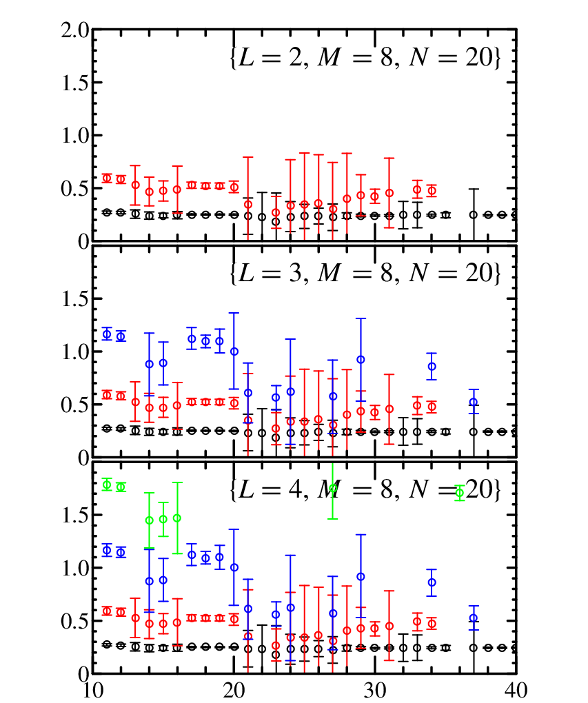
We demonstrate this approach using the smallest smearing parameter (0.5) smeared-point correlator. There are a few parameters in the linear prediction method which we can tune: the number of desired states , the number of time slices used to predict the later time point , and the order of the polynomial . In this work, we will show a selection of the better choices in these degrees of freedom. Figure 5 shows the effective mass plot for from a single Gaussian smeared-point correlator with fixed parameters and . The excited states are consistent with each other as one increases the value of . Since we have used a large value of to form the polynomial, each point uses information extracted from 20 timeslices. Thus, one does not need a large plateau to determine the final mass. One also notes that since we only use a single correlator to extract multiple states, the multiple states will be correlated; that is, large errors on higher-excited states will make the ground state noisy as well. A future improvement would naturally be to extend this approach to multiple correlators.
III.2 Variational Method
Variational method [23, 24] is a powerful tool for extracting multi-excited states in lattice QCD. We construct an spectrum correlation matrix, , where each element of the matrix is a correlator composed from different smeared sources or operators and . Then we consider the generalized eigenvalue problem
| (20) |
where determines the range of validity of our extraction of the lowest eigenstates. If is too large, the highest-lying states will have exponentially decreased too far to have good signal-to-noise ratio; if is too small, many states above the we can determine will contaminate our extraction. Over some intermediate range in , we should find consistent results.
If the eigenvector for this system is , and goes from 1 to . Thus the correlation matrix can be approximated as
| (21) |
with eigenvalues
| (22) |
by solving
| (23) |
Further analysis on the principal correlators, , reveals information on the energy levels, .
The results from the linear prediction approach in Sec. II.1 are compared with the variational method ( with smearing parameter ranging 0.5–3.5), as shown in Fig. 6. Here we shift time with respect to the linear prediction plot by 10 to have a better comparison with the plateau region from the variational method. For the ground state, the numbers are consistent with the result from the variational approach, including the size of the error bar. This is remarkable, given that the amount of input information is a factor of 16 less in the linear prediction approach. The first-excited state is consistent but has larger error bar, which is no surprise. As for the second-excited state, it seems to be consistent with the variational ones but definitely needs more statistics. The third-excited state is much larger than expected from the variational approach, which might be caused by contamination from even higher excited states.

IV Conclusions
The determination of the physical properties of the excited-state hadrons is currently of great interest due to the construction of the 12 GeV upgrade at Jefferson Lab, where such properties will be measured experimentally. Lattice QCD methods have the potential to predict these properties, provided they can be extracted from the exponential time series, called correlation functions, computed in Monte Carlo simulations. In this work, we demonstrate a powerful, yet easy to use, black-box method for analyzing one or more correlation functions and extracting information about excited states. It can easily be adapted to various choices of boundary conditions and discretizations. While the method can be used by itself to estimate physical properties of excited hadrons, we anticipate that it will also be useful as a method for generating initial guesses for nonlinear least-squares minimizers.
Acknowledgments
Computations were performed on clusters at Jefferson Lab with time awarded under the U.S. DOE’s National Computational Infrastructure for Lattice Gauge Theory (USQCD), using the Chroma software suite [47] developed under DOE’s Scientific Discovery through Advanced Computing initiative. This work was supported by U.S. NSF grants PHY-0556243 and PHY-0801068. Authored by Jefferson Science Associates, LLC under U.S. DOE Contract No. DE-AC05-06OR23177. The U.S. Government retains a non-exclusive, paid-up, irrevocable, world-wide license to publish or reproduce this manuscript for U.S. Government purposes.
Appendix A General effective mass solution for , 3, and 4
A.1 General solution for
To reduce the problem, we pre-multiply by two factors of the bi-diagonal matrices of Eq. (4) to find the reduced equation . By introducing the auxiliary quantities:
| (24) | |||||
| (25) |
the reduced system becomes:
| (26) | |||||
| (27) | |||||
| (28) | |||||
| (29) |
The first half of the equations, Eqs. (26) and (27), involve both the amplitudes and the energies but the second half involve only the energies. It will be true for any , in general, that the last equations can be solved first to find all the energies. Once all the energies are known, the first equations form a square upper triangular system that can be solved efficiently by backward substitution to find the amplitudes.
To see that Eqs. (26)–(29) yield the known solution [28], first substitute Eq. (25) and eliminate from Eqs. (28)–(29) to find
| (30) |
where we note that the l.h.s. is the determinant of a Hankel matrix or perhaps the minor of a larger Hankel matrix. After substituting Eq. (24), this gives the known quadratic equation
| (31) |
Note that this can also be written
| (32) |
where the coefficients are not determinants of Hankel matrices but minors of a single Hankel matrix. So, it can be written even more compactly as
| (33) |
where the left block is a Hankel matrix and the right block is a Vandermonde matrix.
A.2 General solution for
Using the auxiliary quantities defined in Eqs. (24) and (25) and a third auxiliary quantity:
| (34) |
the reduced system of equations for is:
| (35) | |||||
| (36) | |||||
| (37) | |||||
| (38) | |||||
| (39) | |||||
| (40) |
Following the procedure of Sec. A.1, substitute Eq. (34) into the last three equations to eliminate and find the (redundant) set of equations
| (41) |
or equivalently
| (42) |
Note the l.h.s. of these three equations are the same as the three coefficients of Eq. (31) after the substitution and thus are minors of a Hankel matrix. Next, substitute Eq. (25) into these equations to eliminate and find the equation
| (43) |
Finally, substituting Eq. (24) will produce a cubic equation in :
| (44) | |||||
The coefficients through are minors of a Hankel matrix and so Eq. (44) can also be written compactly as
| (45) |
The cubic equation can be solved using the method of Scipione del Ferro and Tartaglia [48].
A.3 General solution for
Defining a fourth auxiliary quantity:
| (46) |
the reduced system of equations for is:
| (47) | |||||
| (48) | |||||
| (49) | |||||
| (50) | |||||
| (51) | |||||
| (52) | |||||
| (53) | |||||
| (54) |
Following the now familiar procedure, substitute Eq. (46) into the last four equations to eliminate and find the (redundant) set of equations:
| (55) | |||||
or as minors of a Hankel matrix:
Substitute Eq. (34) and eliminate to find the next set of (redundant) set of equations:
| (70) | |||||
or as minors of a Hankel matrix:
Again, note that the LHS of these four equations are the same as the four coefficients of Eq. (44) after the same substitution . Next, substitute Eq. (25) and eliminate to find the equation
| (84) | |||||
As in Eqs. (30) and (43) the l.h.s. can be written as a determinant of a Hankel matrix of ’s:
| (85) |
Finally, substituting Eq. (24) produces a quartic equation in :
| (86) | |||||
As before, the coefficients though are minors of a Hankel matrix of ’s, so this equation can be written:
| (87) |
The quartic equation can be solved using the method of Ferrari [48].
Appendix B Solution for examples of
B.1 Solution for
The nonlinear equations to solve has a block structure:
| (88) |
Here, the indices for , and are in the ranges , and . To reduce the system we extend Eq. (4) to block form with identical blocks on the diagonal. The reduced equations are
| (89) | |||||
| (90) | |||||
| (91) | |||||
where we have added an additional index to the auxiliary quantities defined in Eqs. (24) and (25). Substituting for in Eqs. (91) and eliminating gives the equation:
| (92) |
where we’ve written the equation as a minor of some matrix, following our experience in Appendix A, yet whose structure is not yet clear. Substituting for gives a quadratic equation in in determinant form:
| (93) |
B.2 Solution for
The reduced system of equations for correlation functions measured on equally spaced time slices to be solved to extract model parameters for states is:
| (94) | |||||
| (95) | |||||
| (96) | |||||
| (97) | |||||
| (98) | |||||
| (99) | |||||
Substituting for and eliminating gives a set of equations in :
Substituting for and eliminating gives a set of equations in :
| (114) |
Substituting for and eliminating gives an equation in :
| (115) |
Substituting for gives a quartic equation in :
| (116) |
B.3 Solution for (K,M,N) = (3,3,4)
The reduced system of equations for correlation functions measured on equally spaced time slices to be solved to extract model parameters for states is:
| (117) | |||||
| (118) | |||||
| (119) | |||||
| (120) | |||||
Substituting for and eliminating gives a set of equations in :
| (121) |
Substituting for and eliminating gives an equation in :
| (122) |
Substituting for gives a cubic equation in :
| (123) |
B.4 Solution for
The reduced system of equations for correlation functions measured on equally spaced time slices to be solved to extract model parameters for states is:
| (124) | |||||
| (125) | |||||
| (126) | |||||
| (127) | |||||
| (128) | |||||
The determinant form of the quartic equation in is
| (129) |
References
- [1] T.-S. H. Lee and L. C. Smith (2006), eprint nucl-th/0611034.
- [2] A. Matsuyama, T. Sato, and T.-S. H. Lee (2006), eprint nucl-th/0608051.
- [3] W. M. Yao et al. (Particle Data Group), J. Phys. G33, 1 (2006).
- [4] C. E. Carlson and N. C. Mukhopadhyay, Phys. Rev. Lett. 67, 3745 (1991).
- [5] O. Krehl, C. Hanhart, S. Krewald, and J. Speth, Phys. Rev. C62, 025207 (2000), eprint nucl-th/9911080.
- [6] S. Sasaki, T. Blum, and S. Ohta, Phys. Rev. D65, 074503 (2002), eprint hep-lat/0102010.
- [7] N. Mathur et al., Phys. Lett. B605, 137 (2005), eprint hep-ph/0306199.
- [8] D. Guadagnoli, M. Papinutto, and S. Simula, Phys. Lett. B604, 74 (2004), eprint hep-lat/0409011.
- [9] D. B. Leinweber, W. Melnitchouk, D. G. Richards, A. G. Williams, and J. M. Zanotti, Lect. Notes Phys. 663, 71 (2005), eprint nucl-th/0406032.
- [10] K. Sasaki, S. Sasaki, and T. Hatsuda, Phys. Lett. B623, 208 (2005), eprint hep-lat/0504020.
- [11] K. Sasaki and S. Sasaki, Phys. Rev. D72, 034502 (2005), eprint hep-lat/0503026.
- [12] T. Burch et al., Phys. Rev. D74, 014504 (2006), eprint hep-lat/0604019.
- [13] S. Basak et al. (2006), eprint hep-lat/0609052.
- [14] B. Sheikholeslami and R. Wohlert, Nucl. Phys. B259, 572 (1985).
- [15] H. Neuberger, Phys. Lett. B417, 141 (1998), eprint hep-lat/9707022.
- [16] D. B. Kaplan, Phys. Lett. B288, 342 (1992), eprint hep-lat/9206013.
- [17] D. B. Kaplan, Nucl. Phys. Proc. Suppl. 30, 597 (1993).
- [18] Y. Shamir, Nucl. Phys. B406, 90 (1993), eprint hep-lat/9303005.
- [19] V. Furman and Y. Shamir, Nucl. Phys. B439, 54 (1995), eprint hep-lat/9405004.
- [20] C. Gattringer, Phys. Rev. D63, 114501 (2001), eprint hep-lat/0003005.
- [21] C. Gattringer, I. Hip, and C. B. Lang, Nucl. Phys. B597, 451 (2001), eprint hep-lat/0007042.
- [22] J. M. Zanotti et al. (CSSM Lattice), Phys. Rev. D65, 074507 (2002), eprint hep-lat/0110216.
- [23] C. Michael, Nucl. Phys. B259, 58 (1985).
- [24] M. Luscher and U. Wolff, Nucl. Phys. B339, 222 (1990).
- [25] G. P. Lepage et al., Nucl. Phys. Proc. Suppl. 106, 12 (2002), eprint hep-lat/0110175.
- [26] Y. Nakahara, M. Asakawa, and T. Hatsuda, Phys. Rev. D60, 091503 (1999), eprint hep-lat/9905034.
- [27] M. Asakawa, T. Hatsuda, and Y. Nakahara, Prog. Part. Nucl. Phys. 46, 459 (2001), eprint hep-lat/0011040.
- [28] G. T. Fleming, in QCD and Numerical Analysis III, edited by A. Boriçi, A. Frommer, B. Joó, A. Kennedy, and B. Pendleton (Springer-Verlag, 2005), no. 47 in Lecture Notes in Computational Science and Engineering, pp. 143–152, ISBN 3-540-21257-4, eprint hep-lat/0403023.
- [29] K. F. Gauss, Comment. Soc. Reg. Sci. Gotten. Recent. 5, 33 (1823).
- [30] G. T. Fleming, S. D. Cohen, H.-W. Lin, and V. Pereyra, PoS LAT2007, 096 (2007).
- [31] S. Basak et al. (Lattice Hadron Physics (LHP)), Phys. Rev. D72, 094506 (2005a), eprint hep-lat/0506029.
- [32] S. Basak et al. (Lattice Hadron Physics (LHP)), Phys. Rev. D72, 074501 (2005b), eprint hep-lat/0508018.
- [33] D. C. Moore and G. T. Fleming, Phys. Rev. D73, 014504 (2006a), eprint hep-lat/0507018.
- [34] D. C. Moore and G. T. Fleming, Phys. Rev. D74, 054504 (2006b), eprint hep-lat/0607004.
- [35] P. Ruffini, Teoria generale delle equazioni, in cui si dimostra impossibile la soluzione algebraica delle equazioni generali di grad superiore al quarto, di Paolo Ruffini (Nella stamperia di S. Tommaso d’Aquino, Bologna, 1799).
- [36] N. H. Abel, J. reine angew. Math. 1, 65 (1826).
- [37] Å. Björck and V. Pereyra, Math. Comput. 24, 893 (1970).
- [38] G. C. F. M. R. de Prony, J. Ecole Poly. 1, 24 (1795), partial translation available in [41].
- [39] G. U. Yule, Phil. Trans. Roy. Soc. Lond. A226, 267 (1927).
- [40] G. Walker, Proc. Roy. Soc. Lond. A131, 518 (1931).
- [41] D. Vandevoorde, Ph.D. thesis, Rensselaer Polytechnic Institute, Troy, New York, USA (1996), http://wwwlib.umi.com/dissertations/fullcit/9806112.
- [42] H. S. Sharatchandra, H. J. Thun, and P. Weisz, Nucl. Phys. B192, 205 (1981).
- [43] C. van den Doel and J. Smit, Nucl. Phys. B228, 122 (1983).
- [44] M. Creutz, Phys. Rev. D35, 1460 (1987).
- [45] S. Syritsyn and J. W. Negele, PoS LAT2007, 078 (2007), eprint 0710.0425.
- [46] A. Walker-Loud et al. (2008), eprint 0806.4549.
- [47] R. G. Edwards and B. Joo (SciDAC), Nucl. Phys. Proc. Suppl. 140, 832 (2005), eprint hep-lat/0409003.
- [48] G. Cardano, Ars Magna (1545), http://en.wikipedia.org/wiki/Cubic_equation.