\numberofauthors

Multiagent Learning in Large Anonymous Games

\alignauthorIan A. Kash
\affaddrComputer Science Dept.
\affaddrCornell University
\alignauthorEric J. Friedman
\affaddrSchool of Operations Research and Information Engineering
\affaddrCornell University
\alignauthorJoseph Y. Halpern
\affaddrComputer Science Dept.
\affaddrCornell University email: kash@cs.cornell.edu email: ejf27@cornell.edu email: halpern@cs.cornell.edu

Abstract.

In large systems, it is important for agents to learn to act effectively, but sophisticated multi-agent learning algorithms generally do not scale. An alternative approach is to find restricted classes of games where simple, efficient algorithms converge. It is shown that stage learning efficiently converges to Nash equilibria in large anonymous games if best-reply dynamics converge. Two features are identified that improve convergence. First, rather than making learning more difficult, more agents are actually beneficial in many settings. Second, providing agents with statistical information about the behavior of others can significantly reduce the number of observations needed.

Keywords:

Multiagent Learning, Game Theory, Large Games, Anonymous Games, Best-Reply Dynamics

\category

I.2.11Artificial IntelligenceDistributed Artificial Intelligence[Multiagent systems] \categoryJ.4Social and Behavioral SciencesEconomics

1. Introduction

Designers of distributed systems are frequently unable to determine how an agent in the system should behave, because optimal behavior depends on the user’s preferences and the actions of others. A natural approach is to have agents use a learning algorithm. Many multiagent learning algorithms have been proposed including simple strategy update procedures such as fictitious play (10), multiagent versions of Q-learning (25), and no-regret algorithms (5).

However, as we discuss in Section 2, existing algorithms are generally unsuitable for large distributed systems. In a distributed system, each agent has a limited view of the actions of other agents. Algorithms that require knowing, for example, the strategy chosen by every agent cannot be implemented. Furthermore, the size of distributed systems requires fast convergence. Users may use the system for short periods of time and conditions in the system change over time, so a practical algorithm for a system with thousands or millions of users needs to have a convergence rate that is sublinear in the number of agents. Existing algorithms tend to provide performance guarantees that are polynomial or even exponential. Finally, the large number of agents in the system guarantees that there will be noise. Agents will make mistakes and will behave in unexpectedly. Even if no agent changes his strategy, there can still be noise in agent payoffs. For example, a gossip protocol will match different agents from round to round; congestion in the underlying network may effect message delays between agents. A learning algorithm needs to be robust to this noise.

While finding an algorithm that satisfies these requirements for arbitrary games may be difficult, distributed systems have characteristics that make the problem easier. First, they involve a large number of agents. Having more agents may seem to make learning harder—after all, there are more possible interactions. However, it has the advantage that the outcome of an action typically depends only weakly on what other agents do. This makes outcomes robust to noise. Having a large number of agents also make it less useful for an agent to try to influence others; it becomes a better policy to try to learn an optimal response. In contrast, with a small number of agents, an agent can attempt to guide learning agents into an outcome that is beneficial for him.

Second, distributed systems are often anonymous (1); it does not matter who does something, but rather how many agents do it. For example, when there is congestion on a link, the experience of a single agent does not depend on who is sending the packets, but on how many are being sent.

Finally, and perhaps most importantly, in a distributed system the system designer controls the game agents are playing. This gives us a somewhat different perspective than most work, which takes the game as given. We do not need to solve the hard problem of finding an efficient algorithm for all games. Instead, we can find algorithms that work efficiently for interesting classes of games, where for us “interesting” means “the type of games a system designer might wish agents to play.” Such games should be “well behaved,” since it would be strange to design a system where an agent’s decisions can influence other agents in pathological ways.

In Section 3, we show that stage learning (9) is robust, implementable with minimal information, and converges efficiently for an interesting class of games. In this algorithm, agents divide the rounds of the game into a series of stages. In each stage, the agent uses a fixed strategy except that he occasionally explores. At the end of a stage, the agent chooses as his strategy for the next stage whatever strategy had the highest average reward in the current stage. We prove that, under appropriate conditions, a large system of stage learners will follow (approximate) best-reply dynamics despite errors and exploration.

For games where best-reply dynamics converge, our theorem guarantees that learners will play an approximate Nash equilibrium. In contrast to previous results where the convergence guarantee scales poorly with the number of agents, our theorem guarantees convergence in a finite amount of time with an infinite number of agents. While the assumption that best-reply dynamics converge is a strong one, many interesting games converge under best-reply dynamics, including dominance solvable games and games with monotone best replies. Marden et al. (17) have observed that convergence of best-reply dynamics is often a property of games that humans design. Moreover, convergence of best-reply dynamics is a weaker assumption than a common assumption made in the mechanism design literature, that the games of interest have dominant strategies (each agent has a strategy that is optimal no matter what other agents do).

Simulation results, presented in Section 4, show that convergence is fast in practice: a system with thousands of agents can converge in a few thousand rounds. Furthermore, we identify two factors that determine the rate and quality of convergence. One is the number of agents: having more agents makes the noise in the systen more consistent so agents can learn using fewer observations. The other is giving agents statistical information about the behavior of other agents; this can speed convergence by an order of magnitude. Indeed, even noisy statistical information about agent behavior, which should be relatively easy to obtain and disseminate, can significantly improve performance.

2. Related Work

One approach to learning to play games is to generalize reinforcement learning algorithms such as Q-learning (25). One nice feature of this approach is that it can handle games with state, which is important in distributed systems. In Q-learning, an agent associates a value with each state-action pair. When he chooses action $a$ in state $s$ , he updates the value $Q(s,a)$ based on the reward he received and the best value he can achieve in the resulting state $s^{\prime}$ ( $\max_{a^{\prime}}Q(s^{\prime},a^{\prime})$ ). When generalizing to multiple agents, $s$ and $a$ become vectors of the state and action of every agent and the $\max$ is replaced by a prediction of the behavior of other agents. Different algorithms use different predictions; for example, Nash-Q uses a Nash equilibrium calculation (15). See (22) for a survey.

Unfortunately, these algorithms converge too slowly for a large distributed system. The algorithm needs to experience each possible action profile many times to guarantee convergence. So, with $n$ agents and $k$ strategies, the naive convergence time is $O(k^{n}$ ). Even with a better representation for anonymous games, the convergence time is still $O(n^{k})$ (typically $k\ll n$ ). There is also a more fundamental problem with this approach: it assumes information that an agent is unlikely to have. In order to know which value to update, the agent must learn the action chosen by every other agent. In practice, an agent will learn something about the actions of the agents with whom he directly interacts, but is unlikely to gain much information about the actions of other agents.

Another approach is no-regret learning, where agents choose a strategy for each round that guarantees that the regret of their choices will be low. Hart and Mas-Colell (13) present such a learning procedure that converges to a correlated equilibrium (21) given knowledge of what the payoffs of every action would have been in each round. They also provide a variant of their algorithm that requires only information about the agent’s actual payoffs (14). However, to guarantee convergence to within $\epsilon$ of a correlated equilibrium requires $O(kn/\epsilon^{2}\log kn)$ , still too slow for large systems. Furthermore, the convergence guarantee is that the distribution of play converges to equilibrium; the strategies of individual learners will not converge. Better results can be achieved in restricted settings. For example, Blum et al. (2) showed that in routing games a continuum of no-regret learners will approximate Nash equilibrium in a finite amount of time.

Foster and Young (7) use a stage-learning procedure that converges to Nash equilibrium for two-player games. Germano and Lugosi (11) showed that it converges for generic $n$ -player games (games where best replies are unique). Young (26) uses a similar algorithm without explicit stages that also converges for generic $n$ -player games. Rather than selecting best replies, in these algorithms agents choose new actions randomly when not in equilibrium. Unfortunately, these algorithms involve searching the whole strategy space, so their convergence time is exponential. Another algorithm that uses stages to provide a stable learning environment is the ESRL algorithm for coordinated exploration (24).

Marden et al. (18, 19) use an algorithm with experimentation and best replies but without explicit stages that converges for weakly acyclic games, where best-reply dynamics converge when agents move one at a time, rather than moving all at once, as we assume here. Convergence is based on the existence of a sequence of exploration moves that lead to equilibrium. With $n$ agents who explore with probability $\epsilon$ , this analysis gives a convergence time of $O(1/\epsilon^{n})$ . Furthermore, the guarantee requires $\epsilon$ to be sufficiently small that agents essentially explore one at a time, so $\epsilon$ needs to be $O(1/n)$ .

There is a long history of work examining simple learning procedures such as fictitious play (10), where each agent makes a best response assuming that each other player’s strategy is characterized by the empirical frequency of his observed moves. In contrast to algorithms with convergence guarantees for general games, these algorithms fail to converge in many games. But for classes of games where they do converge, they tend to do so rapidly. However, most work in this area assumes that the actions of agents are observed by all agents, agents know the payoff matrix, and payoffs are deterministic. A recent approach in this tradition is based on the Win or Learn Fast principle, which has limited convergence guarantees but often performs well in practice (4).

There is also a body of empirical work on the convergence of learning algorithms in multiagent settings. Q-learning has had empirical success in pricing games (23), $n$ -player cooperative games (6), and grid world games (3). Greenwald at al. (12) showed that a number of algorithms, including stage learning, converge in a variety of simple games. Marden et al. (19) found that their algorithm converged must faster in a congestion game than the theoretical analysis would suggest. Our theorem suggests an explanation for these empirical observations: best-reply dynamics converge in all these games. While our theorem applies directly only to stage learning, it provides intuition as to why algorithms that learn “quickly enough” and change their behavior “slowly enough” rapidly converge to Nash equilibrium in practice.

3. Theoretical Results

3.1. Large Anonymous Games

We are interested in anonymous games with countably many agents. Assuming that there are countably many agents simplifies the proofs; it is straightforward to extend our results to games with a large finite number of agents. Our model is adapted from that of (1). Formally, a large anonymous game is characterized by a tuple $\Gamma=(\mathbb{N},A,P,\Pr)$ .

•

$\mathbb{N}$ is the countably infinite set of agents.
•

$A$ is a finite set of actions from which each agent can choose (for simplicity, we assume that each agent can choose from the same set of actions).
•

$\Delta(A)$ , the set of probability distributions over $A$ , has two useful interpretations. The first is as the set of mixed actions. For $a\in A$ we will abuse notation and denote the mixed action that is $a$ with probability 1 as $a$ . In each round each agent chooses one of these mixed actions. The second interpretation of $\rho\in\Delta(A)$ is as the fraction of agents choosing each action $a\in A$ . This is important for our notion of anonymity, which says an agent’s utility should depend only on how many agents choose each action rather than who chooses it.
•

$G=\{g:\mathbb{N}\rightarrow\Delta(A)\}$ is the set of (mixed) action profiles (i.e. which action each agent chooses). Given the mixed action of every agent, we want to know the fraction of agents that end up choosing action $a$ . For $g\in G$ , let $g(i)(a)$ denote the probability with which agent $i$ plays $a$ according to $g(i)\in\Delta(A)$ . We can then express the fraction of agents in $g$ that choose action $a$ as $\lim_{n\rightarrow\infty}(1/n)\sum_{i=0}^{n}g(i)(a)$ , if this limit exists. If the limit exists for all actions $a\in A$ , let $\rho_{g}\in\Delta(A)$ give the value of the limit for each $a$ . The profiles $g$ that we use are all determined by a simple random process. For such profiles $g$ , the strong law of large numbers (SLLN) guarantees that with probability 1 $\rho_{g}$ is well defined. Thus it will typically be well defined (using similar limits) for us to talk about the fraction of agents who do something.
•

$P\subset\mathbb{R}$ is a finite set of payoffs agents can receive.
•

$\Pr:A\times\Delta(A)\rightarrow\Delta(P)$ denotes the distribution over payoffs that results when the agent performs action $a$ and other agents follow action profile $\rho$ . We use a probability distribution over payoffs rather than a payoff to model the fact that agent payoffs may change even if no agent changes his strategy. The expected utility of an agent who performs mixed action $s$ when other agents follow action distribution $\rho$ is $u(s,\rho)=\sum_{a\in A}\sum_{p\in P}ps(a)\Pr_{a,\rho}(p)$ . Our definition of $\Pr$ in terms of $\Delta(A)$ rather than $G$ ensures the the game is anonymous. We further require that $\Pr$ (and thus $u$ ) be Lipschitz continuous.¹¹ 1 Lipschitz continuity imposes the additional constraint that there is some constant $K$ such that $|\Pr(a,\rho)-\Pr(a,\rho^{\prime})|/||\rho-\rho^{\prime}||_{1}\leq K$ for all $\rho$ and $\rho^{\prime}$ . Intuitively, this ensures that the distribution of outcomes doesn’t change “too fast.” This is a standard assumption that is easily seen to hold in the games that have typically been considered in the literature. For definiteness, we use the L1 norm as our notion of distance when specifying continuity (the L1 distance between two vectors is the sum of the absolute values of the differences in each component). Note that this formulation assumes all agents share a common utility function.

An example of a large anonymous game is one where, in each round, each agent plays a two-player game against an opponent chosen at random. Then $A$ is the set of actions of the two-player game and $P$ is the set of payoffs of the game. Once every agent chooses an action, the distribution over actions is characterized by some $\rho\in\Delta(A)$ . Let $p_{a,a^{\prime}}$ denote the payoff for the agent if he plays $a$ and the other agent plays $a^{\prime}$ . Then the utility of mixed action $s$ given distribution $\rho$ is

u(s,\rho)=\sum_{a,a^{\prime}\in A^{2}}s(a)\rho(a^{\prime})p_{a,a^{\prime}}.

3.2. Best-Reply Dynamics

Given a game $\Gamma$ and an action distribution $\rho$ , a natural goal for an agent is to play the action that maximizes his expected utility with respect to $\rho$ : $\argmax_{a\in A}u(a,\rho)$ . We call such an action a best reply to $\rho$ . In a practical amount of time, an agent may have difficulty determining which of two actions with close expected utilities is better, so we will allow agents to choose actions that are close to best replies. If $a$ is a best reply to $\rho$ , then $a^{\prime}$ is an $\eta$ -best reply to $\rho$ if $u(a^{\prime},\rho)+\eta\geq u(a,\rho)$ . There may be more than one $\eta$ -best reply; we denote the set of $\eta$ -best replies $\mathit{ABR}_{\eta}(\rho)$ .

We do not have a single agent looking for a best reply; every agent is trying to find a one at the same time. If agents start off with some action distribution $\rho_{0}$ , after they all find a best reply there will be a new action distribution $\rho_{1}$ . We assume that $\rho_{0}(a)=1/|A|$ (agents choose their initial strategy uniformly at random), but our results apply to any distribution used to determine the initial strategy. We say that a sequence $(\rho_{0},\rho_{1},\ldots)$ is an $\eta$ -best-reply sequence if the support of $\rho_{i+1}$ is a subset of $\mathit{ABR}_{\eta}(\rho_{i})$ ; that is $\rho_{i+1}$ gives positive probability only to approximate best replies to $\rho_{i}$ . A $\eta$ best-reply sequence converges if there exists some $t$ such that for all $t^{\prime}>t$ , $\rho_{t^{\prime}}=\rho_{t}$ . Note that this is a particularly strong notion of convergence because we require the $\rho_{t}$ to converge in finite time and not merely in the limit. A game may have infinitely many best-reply sequences, so we say that approximate best-reply dynamics converge if there exists some $\eta>0$ such that every $\eta$ -best-reply sequence converges. The limit distribution $\rho_{t}$ determines a mixed strategy that is an $\eta$ -Nash equilibrium.

Our theorem shows that learners can successfully learn in large anonymous games where approximate best-reply dynamics converge. The number of stages needed to converge is determined by the number of best replies needed before the sequence converges. It is possibly to design games that have long best-reply sequences, but it practice most games have short sequences. One condition that guarantees this is if $\rho_{0}$ and all the degenerate action distributions $a\in A$ (i.e., distributions that assign probability 1 to some $a\in A$ ) have unique best replies. In this case, there can be at most $|A|$ best replies before equilibrium is reached. Furthermore, in such games the distinction between $\eta$ -best replies and best replies is irrelevant; for sufficiently small $\eta$ , a $\eta$ -best reply is a best reply. It is not hard to show that the property that degenerate strategies have unique best replies is generic; it holds for almost every game.

3.3. Stage Learners

An agent who wants to find a best reply may not know the set of payoffs $P$ , the mapping from actions to distributions over payoffs $\Pr$ , or the action distribution $\rho$ (and, indeed, $\rho$ may be changing over time), so he will have to use some type of learning algorithm to learn it. Our approach is to divide the play of the game into a sequence of stages. In each stage, the agent almost always plays some fixed action $a$ , but also explores other actions. At the end of the stage, he chooses a new $a^{\prime}$ for the next stage based on what he has learned. An important feature of this approach is that agents maintain their actions for the entire stage, so each stage provides a stable environment in which agents can learn. To simplify our results, we specify a way of exploring and learning within a stage (originally described in (9)), but our results should generalize to any “reasonable” learning algorithm used to learn within a stage. (We discuss what is “reasonable” in Section 5.) In this section, we show that, given a suitable parameter, at the each stage most agents will have learned a best reply to the environment of that stage.

Given a game $\Gamma$ , in each round $t$ agent $i$ needs to select a mixed action $s_{i,t}$ . Our agents use strategies that we denote $a_{\epsilon}$ , for $a\in A$ , where $a_{\epsilon}(a)=1-\epsilon$ and $a_{\epsilon}(a^{\prime}\neq a)=\epsilon/(|A|-1)$ . Thus, with $a_{\epsilon}$ , an agent almost always plays $a$ , but with probability $\epsilon$ explores other strategies uniformly at random. Thus far we have not specified what information an agent can use to choose $s_{i,t}$ . Different games may provide different information. All that we require is that an agent know all of his previous actions and his previous payoffs. More precisely, for all $t^{\prime}<t$ , he knows his action $a_{t^{\prime}}(i)$ (which is determined by $s_{i,t^{\prime}}$ ) and his payoffs $p_{t^{\prime}}(i)$ (which is determined by $\Pr(a_{i,t^{\prime}},\rho_{t^{\prime}})$ , where $\rho_{t^{\prime}}$ is the action distribution for round $t^{\prime}$ ; note that we do not assume that the agent knows $\rho_{t^{\prime}}$ .) Using this information, we can express the average value of an action over the previous $\tau=\lceil 1/\epsilon^{2}\rceil$ rounds (the length of a stage).²² 2 The use of the exponent 2 is arbitrary. We require only that the expected number of times a strategy is explored increases as $\epsilon$ decreases. Let $H(a,i,t)=\{t-\tau\leq t^{\prime}<t~|~a_{t^{\prime}}(i)=a\}$ be the set of recent rounds in which $a$ was played by $i$ . Then the average value is $V(a,i,t)=\sum_{t^{\prime}\in H(a,i,t)}p_{t^{\prime}}(i)/|H(a,i,t)|$ if $|H(a,i,t)|>0$ and 0 otherwise. While we need the value of $H$ only at times that are multiples of $\tau$ , for convenience we define it for arbitrary times $t$ .

We say that an agent is an $\epsilon$ -stage learner if he chooses his actions as follows. If $t=0$ , $s_{t}$ is chosen at random from $\{a_{\epsilon}~|~a\in A\}$ . If $t$ is a nonzero multiple of $\tau$ , $s_{i,t}=a(i,t)_{\epsilon}$ where $a(i,t)=\argmax_{a\in A}V(a,i,t)$ . Otherwise, $s_{i,t}=s_{i,t-1}$ . Thus, within a stage, his mixed action is fixed and at the end of a stage he updates it to use the action with the highest average value during the previous stage.

The evolution of a game played by stage learners is not deterministic; each agent chooses a random $s_{i,0}$ and the sequence of $a_{t}(i)$ and $p_{t}(i)$ he observes is also random. However, with a countably infinite set of agents, we can use the SLLN to make statements about the overall behavior of the game. Let $g_{t}(i)=s_{i,t}$ . A run of the game consists of a sequence of triples $(g_{t},a_{t},p_{t})$ . The SLLN guarantees that with probability 1 the fraction of agents who choose a strategy $a$ in $a_{t}$ is $\rho_{g_{t}}(a)$ . Similarly, the fraction of agents who chose $a$ in $a_{t}$ that receive payoff $p$ will be $\Pr(a,\rho_{g_{t}})(p)$ with probability 1.

To make our notion of a stage precise, we refer to the sequence of tuples $(g_{n\tau},a_{n\tau},p_{n\tau})\ldots(g_{(n+1)\tau-1},a_{(n+1)\tau-1},p_{(n+1)\tau-1})$ as stage $n$ of the run. During stage $n$ there is a stationary action distribution that we denote $\rho_{g_{n\tau}}$ . If $s_{i,(n+1)\tau}=a_{\epsilon}$ and $a\in\mathit{ABR}_{\eta}(g_{n\tau})$ , then we say that agent $i$ has learned an $\eta$ -best reply during stage $n$ of the run. As the following lemma shows, for sufficiently small $\epsilon$ , most agents will learn an $\eta$ -best reply.

Lemma 3.1.

For all large anonymous games $\Gamma$ , action profiles, approximations $\eta>0$ , and probabilities of error $e>0$ , there exists an $\epsilon^{*}>0$ such that for $\epsilon<\epsilon^{*}$ and all $n$ , if all agents are $\epsilon$ -stage learners, then at least a $1-e$ fraction of agents will learn an $\eta$ -best reply during stage $n$ .

Proof.

(Sketch) On average, an agent using strategy $a_{\epsilon}$ plays action $a$ $(1-\epsilon)\tau$ times during a stage and plays all other actions $\epsilon\tau/(n-1)$ times each. For $\tau$ large, the realized number of times played will be close to the expectation value with high probability. Thus, if $\epsilon\tau$ is sufficiently large, then the average payoff from each action will be exponentially close to the true expected value (via a standard Hoeffding bound on sums of i.i.d. random variables), and thus each the learner will correctly identify an action with approximately the highest expected payoff with probability at least $1-e$ . By the SLLN, at least a $1-e$ fraction of agents will learn an $\eta$ -best reply. A detailed version of this proof in a more general setting can be found in (9). ∎

3.4. Convergence Theorem

Thus far we have defined large anonymous games where approximate best-reply dynamics converge. If all agents in the game are $\epsilon$ -stage learners, then the sequence $\hat{\rho}_{0},\hat{\rho}_{1},\ldots$ of action distributions in a run of the game is not a best-reply sequence, but it is close. The action used by most agents most of the time in each $\hat{\rho}_{n}$ is the action used in $\rho_{n}$ for some approximate best reply sequence.

In order to prove this, we need to define “close.” Our definition is based on the error rate $e$ and exploration rate $\epsilon$ that introduces noise into $\hat{\rho}_{n}$ . Intuitively, distribution $\hat{\rho}$ is close to $\rho$ if, by changing the strategies of an $e$ fraction of agents and having all agents explore an $\epsilon$ fraction of the time, we can go from an action profile with corresponding action distribution $\rho$ to one with corresponding distribution $\hat{\rho}$ . Note that this definition will not be symmetric.

In this definition, $g$ identifies what (pure) action each agent is using that leads to $\rho$ , $g^{\prime}$ allows an $e$ fraction of agents to use some other action, and $\hat{g}$ incorporates the fact that each agent is exploring, so each strategy is an $a_{\epsilon}$ (the agent usually plays $a$ but explores with probability $\epsilon$ ).

Definition 3.2.

Action distribution $\hat{\rho}$ $(e,\epsilon)$ -close to $\rho$ if there exist $g$ , $g^{\prime}$ , and $\hat{g}\in G$ such that:

•

$\rho=\rho_{g}$ and $\hat{\rho}=\rho_{\hat{g}}$ ;
•

$g(i)\in A$ for all $i\in\mathbb{N}$ ;
•

$||\rho_{g}-\rho_{g^{\prime}}||_{1}\leq 2e$ (this allows an $e$ fraction of agents in $g^{\prime}$ to play a different strategy from $g$ );
•

for some $\epsilon^{\prime}\leq\epsilon$ , if $g^{\prime}(i)=a$ then $\hat{g}(i)=a_{\epsilon^{\prime}}$ .

The use of $\epsilon^{\prime}$ in the final requirement ensures that if two distributions are $(e,\epsilon)$ -close then they are also $(e^{\prime},\epsilon^{\prime})$ -close for all $e^{\prime}\geq e$ and $\epsilon^{\prime}\geq\epsilon$ . As an example of the asymmetry of this definition, $a_{\epsilon}$ is $(0,\epsilon)$ close to $a$ , but the reverse is not true. While $(e,\epsilon)$ -closeness is a useful distance measure for our analysis, it is an unnatural notion of distance for specifying the continuity of $u$ , where we used the L1 norm. The following simple lemma shows that this distinction is unimportant; if $\hat{\rho}$ is sufficiently $(e,\epsilon)$ -close to $\rho$ then it is close according to the L1 measure as well.

Lemma 3.3.

If $\hat{\rho}$ is $(e,\epsilon)$ -close to $\rho$ , then $||\hat{\rho}-\rho||_{1}\leq 2(e+\epsilon)$ .

Proof.

Since $\hat{\rho}$ is $(e,\epsilon)$ -close to $\rho$ , there exist $g$ , $g^{\prime}$ , and $\hat{g}$ as in Definition 3.2. Consider the distributions $\rho_{g}=\rho$ , $\rho_{g^{\prime}}$ , and $\rho_{\hat{g}}=\hat{\rho}$ . We can view these three distributions as vectors, and calculate their L1 distances. By Definition 3.2, $||\rho_{g}-\rho_{g^{\prime}}||_{1}\leq 2e$ . $||\rho_{g^{\prime}}-\rho_{\hat{g}}||_{1}\leq 2\epsilon$ because an $\epsilon$ fraction of agents explore. Thus by the triangle inequality, the L1 distance between $\rho$ and $\hat{\rho}$ is at most $2(e+\epsilon)$ . ∎

We have assumed that approximate best reply sequences of $\rho_{n}$ converge, but during a run of the game agents will actually be learning approximate best replies to $\hat{\rho}_{n}$ . The following lemma shows that this distinction does not matter if $\rho$ and $\hat{\rho}$ are sufficiently close.

Lemma 3.4.

For all $\eta$ there exists a $d_{\eta}$ such that if $\hat{\rho}$ is $(e,\epsilon)$ -close to $\rho$ , $e>0$ , $\epsilon>0$ , and $e+\epsilon<d_{\eta}$ then $\mathit{ABR}_{(\eta/2)}(\hat{\rho})\subseteq\mathit{ABR}_{\eta}(\rho)$ .

Proof.

Let $K$ be the maximum of the Lipschitz constants for all $u(a,\cdot)$ and $d_{\eta}=\eta/(8K)$ . Then for all $\hat{\rho}$ that are $(e,\epsilon)$ -close to $\rho$ and all $a$ , $|u(a,\hat{\rho}-u(a,\rho)|\leq||\hat{\rho}-\rho||_{1}K\leq 2\eta/(8K)K=\eta/4$ by Lemma 3.3.

Let $a\notin\mathit{ABR}_{\eta}(\rho)$ and $a^{\prime}\in\argmax_{a^{\prime}\in\mathit{ABR}_{\eta}(\rho)}u(a^{\prime},\hat{\rho})$ . Then $u(a,\rho)+\eta<u(a^{\prime},\rho)$ . Combining this with the above gives $u(a,\hat{\rho})+\eta/2<u(a^{\prime},\hat{\rho})$ . Thus $a\notin\mathit{ABR}_{\eta/2}(\hat{\rho})$ . ∎

Lemmas 3.1 and 3.4 give requirements on $(e,\epsilon)$ . In the statement of the theorem, we call $(e,\epsilon)$ $\eta$ -acceptable if they satisfy the requirements of both lemmas for $\eta/2$ and all $\eta$ -best-reply sequences converge in $\Gamma$ .

Theorem 3.5.

Let $\Gamma$ be a large anonymous game where approximate best-reply dynamics converge and let $(e,\epsilon)$ be $\eta$ -acceptable for $\Gamma$ . If all agents are $\epsilon$ -stage learners then, for all runs, there exists an $\eta$ -best-reply sequence $\rho_{0},\rho_{1},\ldots$ such that in stage $n$ at least a $1-e$ fraction will learn a best reply to $\rho_{n}$ with probability 1.

Proof.

$\rho_{0}=\hat{\rho_{0}}$ , so $\hat{\rho_{0}}$ is $(e,\epsilon)$ -close to $\rho$ . Assume $\hat{\rho}_{n}$ is $(e,\epsilon)$ -close to $\rho$ . By Lemma 3.1 at least a $1-e$ fraction will learn a $\eta/2$ -best reply to $\hat{\rho}_{n}$ . By Lemma 3.4, this is a $\eta$ -best reply to $\rho_{n}$ . Thus $\hat{\rho}_{n+1}$ will be $(e,\epsilon)$ -close to $\rho_{n+1}$ . ∎

Theorem 3.5 guarantees that after a finite number of stages, agents will be close to an approximate Nash equilibrium profile. Specifically, $\hat{\rho}_{n}$ will be $(e,\epsilon)$ -close to an $\eta$ -Nash equilibrium profile $\rho_{n}$ . Note that this means that $\hat{\rho}_{n}$ is actually an $\eta^{\prime}$ -Nash equilibrium for a larger $\eta^{\prime}$ that depends on $\eta$ , $e$ , $\epsilon$ , and the Lipschitz constant $K$ .

Our three requirements for a practical learning algorithm were that it require minimal information, converge quickly in a large system, and be robust to noise. Stage learning requires only that an agent know his own payoffs, so the first condition is satisfied. Theorem 3.5 shows that it satisfies the other two requirements. Convergence is guaranteed in a finite number of stages. While the number of stages depends on the game, in Section 3.2 we argued that in many cases it will be quite small. Finally, robustness comes from tolerating an $e$ fraction of errors. While in our proofs we assumed these errors were due to learning, the analysis is the same if some of this noise is from other sources such as churn (agents entering and leaving the system) or agents making errors. We discuss this issue more in Section 5.

4. Simulation Results

Theorem 3.5 guarantees convergence for a sufficiently small exploration probability $\epsilon$ , but decreasing $\epsilon$ also increases $\tau$ , the length of a stage. Increasing the length of a stage means that agents take longer to reach equilibrium, so for stage learning to be practical, $\epsilon$ needs to be relatively large. To show that $\epsilon$ can be large in practice, we tested populations of stage learners in a number of games where best reply dynamics converge and experienced convergence with $\epsilon$ between $0.01$ and $0.05$ . This allows convergence within a few thousand rounds in many games. While our theorem applies only to stage learning, the analysis provides intuition as to why a reasonable algorithm that changes slowly enough that other learners have a chance to learn best replies should converge as well. To test a very different type of algorithm, we also implemented the no-regret learning algorithm of Hart and Mas-Collell (14). This algorithm also quickly converged close to Nash equilibrium, although in many games it did not converge as closely as stage learning.

Our theoretical results make two significant predictions about factors that influence the rate of convergence. Lemma 3.1 tells us that the length of a stage is determined by the number of times each strategy needs to be explored to get an accurate estimate of its value. Thus the amount of information provided by each observation has a large effect on the rate of convergence. For example, in a random matching game, an agents payoff provides information about the strategy of one other agent. On the other hand, if he receives his expected payoff for being matched, a single observation provides information about the entire distribution of strategies. In the latter case the agent can learn with many fewer observations.

A related prediction is that having more agents will lead to faster convergence, particularly in games where payoffs are determined by the average behavior of other agents, because variance in payoffs due to exploration and mistakes decreases as the number of agents increases. Our experimental results illustrate both of these phenomena.

We tested the learning behavior of stage learners and no-regret learners in a number of games, including prisoner’s dilemma, a climbing game (6), the congestion game described in (12) with both ACP and serial mechanisms, and two different contribution games (called a Diamond-type search model in (20)). We implemented payoffs both by randomly matching players and by giving each player what his expected payoff would have been had he been randomly matched (some payoffs were adjusted to make the games symmetric). Results were similar across the different games, so we report only the results for a contribution game.

In the contribution game, agents choose strategies from 0 to 19, indicating how much effort they contribute to a collective enterprise. The value to an agent depends on how much he contributes, as well as how much other agents contribute. If he contributes $x$ and the contribution of the other agents is $y$ , then his utility is $2xy-c(x)$ , where $c(0)=0$ , $c(1)=1$ , $c(x)=(x-1)^{2}$ for $x\in 2,\ldots,8$ and $c(x)=x^{2}+2n$ for $x>8$ . We considered two versions of this game. In the first, $y$ is determined by the average strategy of the other agents. In the second, $y$ is determined by randomly matching the agent with another agent.

Our implementation of stage learners is as described in Section 3.3, with $\epsilon=0.05$ when $y$ is determined by the average and $\epsilon=0.01$ when $y$ is determined by random matching. Rather than taking the length of stage $\tau$ as $1/\epsilon^{2}$ , we set $\tau=250$ and $2000$ , respectively; this gives better performance. Our implementation of no-regret learners is based on that of Hart and Mas-Colell (14), with improvements suggested by Greenwald et al. (12).

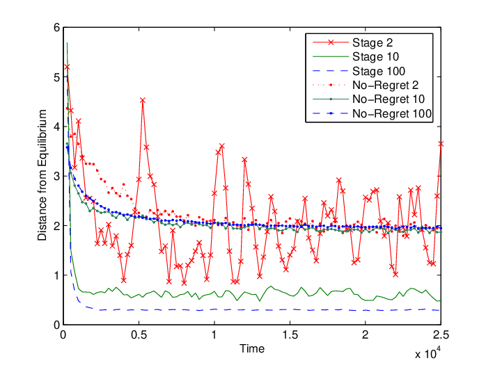
Refer to caption — Figure 1. Convergence with the average

Figure 1 shows the results for learners in the version of the game where $y$ is the average strategy of other agents. Each curve shows the distance from equilibrium as a function of the number of rounds of a population of agents of a given size using a given learning algorithm. The results were averaged over 10 runs. Since the payoffs for nearby strategies are close, we want our notion of distance to take into account that agents playing 7 are closer to equilibrium (8) than those playing zero. Therefore, we consider the expected distance of $\rho$ from equilibrium: $\sum_{a}\rho(a)|a-8|$ . To determine $\rho$ , we counted the number of times each action was over the length of a stage, so in practice the distance will never be zero due to mistakes and exploration. For ease of presentation, the graph shows only populations of size up to 100; similar results were obtained for populations up to 5000 agents.

For stage learning, increasing the population size has a dramatic impact. With two agents, mistakes and best replies to the results of these mistakes cause behavior to be quite chaotic. With ten agents, agents successfully learn, although mistakes and suboptimal strategies are quite frequent. With one hundred agents, all the agents converge quickly to equilibrium strategies and mistakes are rare; almost all of the distance from equilibrium is due to exploration.

No-regret learning also converges quickly, but the “quality” of convergence (how close we get to equilibrium) is not as high. The major problem is that a significant fraction of agents play near-optimal actions rather than optimal action. This may have a number of causes. First, the guarantee is that the asymptotic value of $\rho$ will be an equilibrium, which allows the short periods that we consider to be far from equilibrium. Second, the quality of convergence depends on $\epsilon$ , so tight convergence may require a much lower rate of exploration and thus a much longer convergence time. Finally, this algorithm is guaranteed to converge only to a correlated equilibrium, which may not be a Nash equilibrium.

Figure 2 shows the results when agent payoffs are determined by randomly matching agents. Even for large numbers of stage learners, convergence is not as tight and takes on the order of ten times longer. This is a result of the information available to agents. When payoffs were determined by the average strategy, a single observation was sufficient to evaluate a strategy, so we could use very short stages. To deal with the noise introduced by random matching we need much longer stages. The number of stages to convergence is similar. Even with longer stages and a large number of agents, mistakes are quite common. Nevertheless agents do successfully learn. The performance of no-regret learners is less affected because they use payoff information from the entire run of the game, while stage learners discard payoff information at the end of each stage.

Convergence in the random-matching game takes approximately 20,000 rounds, which is too slow for many applications. If a system design requires this type of matching, this makes learning problematic. However, the results of Figure 1 suggest that the learning could be done much faster if the system designer could supply agents with more information. This suggests that collecting statistical information about the behavior of agents may be a critical feature for ensuring fast convergence. If agents know enough about the game to determine their expected payoffs from this statistical information, then they can directly learn, as in Figure 1. Even with less knowledge about the game, statistical information can still speed learning, for example, by helping an agent determine whether the results of exploring an action were typical or due to the other agent using a rare action.

5. Discussion

While our results show that a natural learning algorithm can learn efficiently in an interesting class of games, there are many further issues that merit exploration.

Other Learning Algorithms

Our theorem assumes that agents use a simple rule for learing within each stage: they average the value of payoffs received. However, there are certainly other rules for estimating the value of an action; any of these can be used as long as the rule guarantees that errors can be made arbitrarily rare given sufficient time. It is also not necessary to restrict agents to stage learning. Stage learning guarantees a stationary environment for a period of time, but such strict behavior may not be needed or practical. Other approaches, such as exponentially discounting the weight of observations (12, 19) or Win or Learn Fast (4) allow an algorithm to focus its learning on recent observations and provide a stable environment in which other agents can learn.

Other Update Rules

In addition to using different algorithms to estimate the values of actions, a learner could also change the way he uses those values to update his behavior. For example, rather than basing his new strategy on only the last stage, he could base it on the entire history of stages and use a rule in the spirit of fictitious play. Since there are games where fictitious play converges but best-reply dynamics do not, this could extend our results to another interesting class of games, as long as the errors in each period do not accumulate over time. Another possibility is to update probabilistically or use a tolerance to determine whether to update (see e.g. (7, 14)). This could allow convergence in games where best-reply dynamics oscillate or decrease the fraction of agents who make mistakes once the system reaches equilibrium.

Model Assumptions

Our model makes several unrealistic assumptions, most notably that there are countably many agents who all share the same utility function. Essentially the same results holds with a large, finite number of agents, adding a few more “error terms”. In particular, since there is always a small probability that every agent makes a mistake at the same time, we can prove only that no more than a $1-e$ fraction of the agents make errors in most rounds, and that agents spending most of their time playing equilibrium strategies.

We have also implicitly assumed that the set of agents is fixed. We could easily allow for churn: agents entering and leaving the system. A reasonable policy for newly-arriving agents is to pick a random $a_{\epsilon}$ to use in the next stage. If all agents do this, it follows that convergence is unaffected: we can treat the new agents as part of the $e$ fraction that made a mistake in the last stage. Furthermore, this tells us that newly arriving agents “catch up” very quickly. After a single stage, new agents are guaranteed to have learned a best reply with probability at least $1-e$ .

Finally, we have assumed that all agents have the same utility function. Our results can easily be extended to include a finite number of different types of agents, each with their own utility function, since the SLLN can be applied to each type of agent. We believe that our results hold even if the set of possible types is infinite. This can happen, for example, if an agent’s utility depends on a valuation drawn from some interval. However, some care is needed to define best-reply sequences in this case.

State

One common feature of distributed systems not addressed in this work is state. For example, in a scrip system where agents pay each other for service using an internal currency or scrip, whether an agent should seek to provide service depends on the amount of money he currently has (8).

In principle, we could extend our framework to games with state: in each stage each agent chooses a policy to usually follow and explores other actions with probability $\epsilon$ . Each agent could then use some off-policy algorithm (one where the agent can learn without controlling the sequence of observations; see (16) for examples) to learn an optimal policy to use in the next stage. One major problem with this approach is that standard algorithms learn too slowly for our purposes. For example, Q-learning (25) typically needs to observe each state-action pair hundreds of times in practice. The low exploration probability means that the expected $|S||A|/\epsilon$ rounds needed to explore each even once for each pair is large. Efficient learning requires more specialized algorithms that can make better use of the structure of a problem, but this also makes providing a general guarantee of convergence more difficult. Another problem is that, even if an agent explores each action for each of his possible local states, the payoff he receives will depend on the states of the other agents and thus the actions they chose. We need some property of the game to guarantees this distribution of states is in some sense “well behaved.”

Despite these concerns, preliminary results suggest that simple learning algorithms work well for games with state. In experiments on a game using the model of a scrip system from (8), we found that a stage-learning algorithm that uses a specialized algorithm for determining the value of actions in each stage converges to equilibrium quickly despite churn and agents learning at different rates.

Mixed Equilibria

Another restriction of our results is that our agents only learn pure strategies. One way to address this is to discretize the mixed strategy space (see e.g. (7)). If one of the resulting strategies is sufficiently close to an equilibrium strategy and best-reply dynamics converge with the discretized strategies, then we expect agents to converge to a near-equilibrium distribution of strategies. We have had empirical success using this approach to learn to play rock-paper-scissors.

Unexpected and Byzantine Behavior

In practice, we expect that not all agents will be trying to learn optimal behavior in a large system. Some agents may simply play some particular (possibly mixed) strategy that they are comfortable with, without trying to learn a better strategy. Others may be learning but with an unanticipated utility function. Whatever their reasons, if these sufficiently few such agents are choosing their strategies i.i.d. from fixed distribtions (or at least fixed for each stage), then our results hold without change. This is because we already allow an $e$ fraction of agents to make arbitrary mistakes, so we can treat these agents as simply mistaken.

Byzantine agents, who might wish to disrupt learning as much as possible, do not fit as neatly into our framework; they need not play the same strategy for an entire stage. However, we expect that since correct agents are randomizing their decisions, a small number of Byzantine agents should not be able to cause many agents to make mistakes.

6. Conclusion

Learning in distributed systems requires algorithms that are scalable to thousands of agents and can be implemented with minimal information about the actions of other agents. Most general-purpose multiagent learning algorithms fail one or both of these requirements. We have shown here that stage learning can be an efficient solution in large anonymous games where approximate best-reply dynamics lead to approximate pure strategy Nash equilibria. Many interesting classes of games have this property, and it is frequently found in designed games. In contrast to previous work, the time to convergence guaranteed by the theorem does not increase with the number of agents. If system designers can find an appropriate game satisfying these properties on which to base their systems, they can be confident that nodes can efficiently learn appropriate behavior.

Our results also highlight two factors that aid convergence. First, having more learners often improves performance. With more learners, the noise introduced into payoffs by exploration and mistakes becomes more consistent. Second, having more information typically improves performance. Publicly available statistics about the observed behavior of agents can allow an agent to learn effectively while making fewer local observations.

Acknowledgements

EF, IK, and JH are supported in part by NSF grant ITR-0325453. JH is also supported in part by NSF grant IIS-0812045 and by AFOSR grants FA9550-08-1-0438 and FA9550-05-1-0055. EF is also supported in part by NSF grant CDI-0835706.

References

[1] M. Blonski. Equilibrium characterization in large anonymous games. Technical report, U. Mannheim, 2001.
[2] A. Blum, E. Even-Dar, and K. Ligett. Routing without regret: on convergence to Nash equilibria of regret-minimizing algorithms in routing games. In Proc 25th ACM Symp. on Principles of Distributed Computing (PODC), pages 45–52, 2006.
[3] M. H. Bowling. Convergence problems of general-sum multiagent reinforcement learning. In 17th Int. Conf. on Machine Learning (ICML 2000), pages 89–94, 2000.
[4] M. H. Bowling and M. M. Veloso. Rational and convergent learning in stochastic games. In 17th Int. Joint Conference on Artificial Intelligence (IJCAI 2001), pages 1021–1026, 2001.
[5] N. Cesa-Bianchi and G. Lugosi. Prediction, Learning and Games. Cambridge University Press, 2006.
[6] C. Claus and C. Boutilier. The dynamics of reinforcement learning in cooperative multiagent systems. In AAAI-97 Workshop on Multiagent Learning, pages 746–752, 1998.
[7] D. P. Foster and P. Young. Regret testing: Learning to play Nash equilibrium without knowing you have an opponent. Theoretical Economics, 1:341–367, 2006.
[8] E. J. Friedman, J. Y. Halpern, and I. A. Kash. Efficiency and Nash equilibria in a scrip system for P2P networks. In Proc. Seventh ACM Conference on Electronic Commerce (EC), pages 140–149, 2006.
[9] E. J. Friedman and S. Shenker. Learning and implementation on the internet. 1998.
[10] D. Fudenberg and D. Levine. Theory of Learning in Games. MIT Press, 1998.
[11] F. Germano and G. Lugosi. Global Nash convergence of Foster and Young’s regret testing. Games and Economic Behavior, 60(1):135–154, July 2007.
[12] A. Greenwald, E. J. Friedman, and S. Shenker. Learning in networks contexts: Experimental results from simulations. Games and Economic Behavior, 35(1-2):80–123, 2001.
[13] S. Hart and A. Mas-Colell. A simple adaptive procedure leading to correlated equilibrium. Econometrica, 68(5):1127–1150, 2000.
[14] S. Hart and A. Mas-Colell. A reinforecement learning procedure leading to correlated equilibrium. In G. Debreu, W. Neuefeind, and W. Trockel, editors, Economic Essays, pages 181–200. Springer, 2001.
[15] J. Hu and M. P. Wellman. Nash Q-learning for general-sum stochastic games. Journal of Machine Learning Research, 4:1039–1069, 2003.
[16] L. P. Kaelbling, M. L. Littman, and A. P. Moore. Reinforcement learning: A survey. J. Artif. Intell. Res. (JAIR), 4:237–285, 1996.
[17] J. R. Marden, G. Arslan, and J. S. Shamma. Connections between cooperative control and potential games. In Proceedings of the 2007 European Control Conference (ECC), 2007.
[18] J. R. Marden, G. Arslan, and J. S. Shamma. Regret based dynamics: convergence in weakly acyclic games. In 6th Int. Joint Conf. on Autonomous Agents and Multiagent Systems (AAMAS), pages 42–49, 2007.
[19] J. R. Marden, H. P. Young, G. Arslan, and J. S. Shamma. Payoff-based dynamics for multi-player weakly acyclic games. SIAM Journal on Control and Optimization, 2008. To appear.
[20] P. Milgrom and J. Roberts. Rationalizability, learning, and equilibrium in games with strategic complement- arities. Econometrica, 58(6):1255–1277, 1900.
[21] M. Osborne and A. Rubenstein. A Course in Game Theory. MIT Press, 1994.
[22] Y. Shoham, R. Powers, and T. Grenager. Multi-agent reinforcement learning: a critical survey. Technical report, Stanford, 2003.
[23] G. Tesauro and J. O. Kephart. Pricing in agent economies using multi-agent Q-learning. Autonomous Agents and Multi-Agent Systems, 5(3):289–304, 2002.
[24] K. Verbeeck, A. Nowé, J. Parent, and K. Tuyls. Exploring selfish reinforcement learning in repeated games with stochastic rewards. Journal of Autonomous Agents and Multi-agent Systems, 14:239–269, 2007.
[25] C. J. Watkins and P. Dayan. Technical note Q-learning. Machine Learning, 8:279–292, 1992.
[26] H. P. Young. Learning by trial and error. Games and Economic Behavior, forthcoming.