Black/White hole radiation from dispersive theories
Abstract
We study the fluxes emitted by black holes when using dispersive field theories. We work with stationary one dimensional backgrounds which are asymptotically flat on both sides of the horizon. The asymptotic fluxes are governed by a Bogoliubov transformation. The fluxes emitted by the corresponding white holes are regular and governed by the inverse transformation. We numerically compute the spectral properties of these fluxes for both sub- and superluminal quartic dispersion. The leading deviations with respect to the dispersionless flux are computed and shown to be governed by a critical frequency above which there is no radiation. Unlike the UV scale governing dispersion, its value critically depends on the asymptotic properties of the background. We also study the flux outside the robust regime. In particular we show that its low-frequency part remains almost thermal but with a temperature which significantly differs from the standard one. Application to four dimensional black holes and Bose Einstein condensates are in preparation.
pacs
04.70.Dy, 04.60.Bc, 43.35.+dI Introduction
In 1981, Unruh showed [1] that the phonon field equation in a nonhomogeneous flow is analogous to that of a relativistic field propagating in a four dimensional curved space-time. He also suggested that this analogy could be used to experiment black hole (BH) radiation in the lab. However, as pointed out in [2], this analogy is limited by the fact that in condensed matter the phonon field becomes dispersive above a certain wave vector, say . Motivated by this remark, Unruh numerically showed that the fluxes emitted by an acoustic black hole are not significantly affected by the dispersive properties of the phonons, at least when , where is the gradient of the fluid velocity at the sonic horizon. [3] Since then, this robustness of the fluxes has been confirmed both by algebraic [4, 5, 6, 7, 8, 9] and numerical [10, 11] techniques.
However, many open questions remain. In particular, little is known about
- •
the exact nature and the precise range of the parameters delimiting the robust regime,
- •
the scaling properties of the leading deviations in the robust regime,
- •
the properties of the fluxes outside this regime, and
- •
the comparison of sub- and superluminal dispersion.
In view of the possibility to detect Hawking radiation in the lab, [12] it is important to provide quantitative estimates of the modifications of the fluxes induced by dispersion. Besides this reason, answering the above questions is also relevant when exploring the consequences on black hole physics due to violations of Lorentz invariance [2, 13, 14, 15, 16] that could stem from (or be related to) quantum gravity. This could be true in particular when considering the signals emitted during the evaporation of light black holes ( Planck mass) that could be produced at the LHC [17].
In this paper, we aim to answer these questions by a two step analysis. First we provide a complete description of the quantum propagation of a dispersive field in stationary black hole geometries. (To our knowledge, this has not been presented anywhere.) Secondly, focussing on quartic dispersion and using numerical methods, we study both the small modifications of the fluxes induced by dispersion when , and the larger modifications when this inequality is not satisfied.
We are planning to extend this work in two directions. First, to Bose condensates, where the phonon field obeys the Bogoliubov-de-Gennes equation which differs from the “scalar” field equation we consider below (this program has been completed during the publication process of the present work [18]) and secondly to 4D black holes, where the gravitational potential induces grey body factors which could play a critical role.
In Sec. II, we present the class of velocity profiles and the stationary mode equation. In Sec. III, we study the algebraic properties of the modes and the Bogoliubov transformation one is dealing with. In Sec. IV, we present our numerical treatment. In Secs. V and VI, we numerically solve the mode equation and interpret the results for sub- and superluminal quartic dispersion respectively. We conclude in Sec. VII.
II The settings
II.1 Velocity profiles
We work in two space-time dimensions and consider stationary black hole geometries. These shall be characterized by the velocity profile :
| (1) |
This expression appears [1] when considering the propagation of low-frequency phonons in a moving fluid whose velocity field is measured in the Galilean frame (not necessarily the lab frame) where only depends on . The sound velocity is assumed to be constant and has been set to . A more general case will be considered in [18]. The above metric possesses an event horizon where the flow becomes supersonic.
When the fluid flows to the left, , and when increases toward the left, one obtains a future (black hole BH) horizon. Had we considered the flow , we would have obtained a white hole (WH) geometry. As we shall see, the spectral properties (in terms of the conserved frequency ) of fluxes emitted by this WH are in one-to-one correspondence with those of the fluxes emitted by the BH governed by . However they differ slightly. It should also be pointed out that, since we only consider dispersive mode equations, see e.g. Eq. (5), in Eq. (1) represents the whole space-time [19], and not only a part of it as would have been the case when using relativistic fields.
We shall also assume that becomes asymptotically constant on both sides of the horizon. The existence of two asymptotic regions is important because one then has well-defined asymptotic modes on both sides, and therefore well-defined particle fluxes. This is particularly relevant for the proposal [20, 21] based on measurements of the long distance correlations [22, 23] between Hawking quanta and their partners propagating on the other side of the horizon.
In order to determine the generic consequences of dispersion, we shall consider a large class of flows. In contrast with the nondispersive case where they play no role, we shall see that the asymptotic properties of are crucial when using nonlinear dispersion relations. This will imply in particular that the inequality is not sufficient to guarantee no significant deviation from the standard fluxes.
The class we shall use generalizes that of [10] and contains profiles of the form
| (2) |
When changing and , , the slope of at the horizon, is fixed, as is the location of the horizon at . When using the 2D massless relativistic theory, the emitted spectrum only depends on . Instead, when using dispersive theories, together with the ratio , both and also affect the properties of the fluxes. Figure 1 shows for several values of and , as a function of .

The power controls the sharpness of the transition from the linear behavior of near the horizon to the asymptotic flat region. For , the transition becomes sharp. When using dispersive theories, sharp transitions give rise to nonadiabatic effects which produce superimposed oscillations [10]. Unless said otherwise, is equal to in the following.
The parameter fixes the asymptotic values of the velocities,
| (3) |
for respectively. When using nonlinear dispersion relations, fixes the critical frequency above which the radiation vanishes. This is relevant because is constrained to be much smaller than in some proposals of experiments [24]. More generally, we shall find that is the most relevant parameter, in that the corrections induced by dispersion are essentially governed by , and not by as one might have expected.
II.2 Dispersive wave equation
In Nature of course, various dispersion relations are found depending on the condensed material used. However, when imposing analyticity in , quartic dispersion relations represent the first two possible deviations from the linear case. (Dissipative theories constitute another class that should be considered separately [25, 26].) In this paper, we shall thus restrict our numerical analysis to
| (4) |
where and are the energy and momentum measured in the frame comoving with the flow.
When working with the metric of Eq. (1) the corresponding wave equation for the velocity potential reads [3]
| (5) |
when assuming that the fluid density is constant. (This restriction will also be removed in [18].) The upper (lower) sign corresponds to super- (sub-) luminal dispersion. The conserved scalar product takes the form
| (6) |
It is independent of the dispersion and it coincides with the standard Klein-Gordon (KG) product evaluated on the preferred time slices specified by dispersion (here ).
Since the flow is stationary, we shall work at fixed (Killing) frequency . Setting in the wave equation yields
| (7) |
As usual, the scalar product is block diagonal in . Therefore, when working with stationary states, all observables will be expressed as sums of observables defined at fixed . More precisely, one should consider the couple of frequencies since opposite values of mix in stationary Bogoliubov transformations. In what follows, to avoid any confusion, is always positive definite.
Before numerically studying the solutions of Eq. (7), it is worth analyzing the enlarged set of solutions and the Bogoliubov transformation one obtains.
We remind the reader that the oscillatory solutions to Eq. (7) can be classified according to the sign of their group velocity in the comoving frame, . In the following we call the modes with left movers and those with the opposite sign right movers. In the absence of dispersion (and for 2D massless fields), these two sectors are decoupled, and the Bogoliubov transformation is particularly simple. When introducing (quartic) dispersion, four independent solutions to Eq. (7) exist. The classification between left and right movers can still be done, but the left-right decoupling is lost. It is worth mentioning that, when considering a varying speed of sound rather than a varying flow-velocity, see e.g. [21], this decoupling is lost even in the long wavelength approximation (i.e. without dispersion). Notice also that one can introduce dispersion in a way that preserves this factorization [4, 27], but these models do not seem to govern condensed matter systems.
III Analytic study
In several aspects, the material presented below closely follows what has been presented in [10]. The novelties are related to the fact that we treated both asymptotic regions on an equal footing. In particular, we establish the complete character of the “in” and “out” mode bases, and we write the unitary Bogoliubov transformation which governs the general case (for stationary, one dimensional, single horizon geometries). Finally, we show how to relate the fluxes emitted by black and white holes.
III.1 Asymptotic solutions
Given our velocity profile, is asymptotically constant in both regions . There, the solutions of Eq. (7) are superpositions of plane waves with constant amplitudes. To characterize a solution, one needs the roots of the asymptotic wave vectors and the amplitudes of the corresponding waves. Owing to the nonlinearity of the dispersion relation, in addition to the oscillatory modes, exponentially growing/decaying modes exist, governed by complex values of .
We first study how to handle these extra modes in the present settings, paying attention to the completeness of the mode basis. To be specific, we concentrate on superluminal cases, and only indicate the (small) differences that arise in subluminal cases.

Let us thus analyze the roots of
| (8) |
for , and for an arbitrary value of the integer . We work with a polynomial form so as to know the number of complex roots of Eq. (8). For everything concerning the real roots, nothing changes if one uses any strictly convex function with a slope equal to 1 for low .
In the subsonic region, , as can be seen in Fig. 2, two real roots exist: and which correspond to a right and a left mover respectively. (Whenever an ambiguity could exist, we shall add a superscript or to designate right or left movers.) pairs of complex conjugated roots also exist, since the equation is real. One thus has roots with a positive imaginary part (which correspond to growing modes to the right) and solutions with a negative imaginary part (decaying modes).
In the supersonic region , for smaller than a critical frequency (we shall compute its value below) there exist four real roots (see Fig. 2), and thus only pairs of complex solutions. In other words, when comparing this with what prevailed in the subsonic region, a pair of growing and decaying modes has been replaced by a couple of oscillatory modes. Such replacements of pairs of modes is a generic feature of QFT in external fields, see the Appendix of [28]. In the present hydrodynamical settings it will occur at all horizons (for both black and white holes). For flows to the left, , the two new real roots both correspond to right movers. Notice that for subluminal dispersion, the replacement occurs the other way around since the four real roots are found where the flow is subsonic.
Now, given that there are roots, the general solution is a superposition of modes. However, when considering the Fourier transform of the field operator, , only a subclass of these should be used. And this subclass is complete in a precise sense we explain below. (To our knowledge, this crucial aspect has not been discussed in the context of acoustic black holes.) To establish the completeness of the mode basis we first need to compute the frequency which is introduced by both sub- and superluminal dispersion, and which will cut off Hawking radiation.
III.2 Maximal frequency

The frequency is the value of where the two extra real roots merge into each other. It is thus reached when the straight line is tangent to , as illustrated in Fig. 3, or equally when is tangent to , where is the square root of the rhs of Eq. (8).
Restricting attention to quartic dispersion, the corresponding value of is
| (9) |
The frequency is then obtained from Eq. (8). It is thus of the form
| (10) |
For , one has . This means that, whatever the value of the dispersion scale , can be arbitrarily small, and in particular it could be even smaller than the temperature one would get in a dispersionless theory.
For subluminal dispersion, the maximal frequency is again defined by the merging of the two extra real roots. In this case it occurs where . In the quartic case the corresponding value of is
| (11) |
Thus is also of the form . For , we again obtain .

Fig. 4 shows the contours of constant in the plane , for sub- and superluminal dispersion. The same value of can be obtained with very different combinations of . As we shall see in Sec. V, the fluxes are highly degenerate on these contours, which means that the corrections with respect to the standard fluxes are essentially governed by .
III.3 Mode orthonormality and mode completeness
To proceed to the canonical quantization, one should use mode bases that are orthonormal and complete. When the background geometry is homogeneous, this is rather easy, even in the presence of dispersion. However, when of Eq. (1) varies and in particular when it characterizes a horizon, it becomes trickier. Let us thus first consider situations where is constant both in space and time.
III.3.1 Homogeneous metrics, -representation
In this case one should exploit the homogeneity and express the field operator in terms of exponentials and creation/destruction operators labelled by (real)
| (12) |
where with given in Eq. (8). In this representation, creation/destruction operators obey the usual commutators . In addition, the modes which multiply these operators in Eq. (12) are orthonormal: their norm, Eq. (6), is , irrespectively of both whether is sub- or supersonic, and the choice of the dispersion relation (8).11 1 In the case of subluminal dispersion, there could exist a maximal value of associated with the vanishing of . In this case, the mode basis is no longer complete in a Fourier sense. To deal with this, one can either work [29] with “regularized” dispersion relations which do not develop imaginary values of , or with a “Bloch waves” perspective [30] where is periodic in -space.
The completeness of the mode basis is needed to verify that the equal time commutator
| (13) |
is satisfied when is given in Eq. (12) and where . In the present representation, the proof is easily obtained by making use of the completeness (in the sense of Fourier analysis) of the exponentials , with real from . It should be stressed that the proof applies to all dispersion relations and to all (constant) values of , both sub- and supersonic.
When considering nonhomogeneous stationary flows one must use the conserved frequency in place of the wave vector to label modes and operators. So, in preparation for this case, let us study the change of representation from to in homogeneous flows.
III.3.2 Homogeneous metrics, the -representation
The above conclusion concerning the completeness character of the modes implies that, in any homogeneous flow, the “extra” (growing and decaying) solutions of the mode equation at fixed must be discarded when quantizing . When the flow is subsonic, using the dispersion relation (8), one should thus discard the growing/decaying modes, whereas when the flow is supersonic, one should discard only modes. Because of this, the change of representation from to should be done separately in sub- and supersonic regions.
Let us first consider the subsonic case where only two real roots exist. For each , one has two modes:
| (14) |
where , , are the two real roots of Eq. (8) describing the right- and left-moving modes. These modes obey Eq. (7) and are orthonormal for the KG product, in the sense of a Dirac distribution . Correspondingly, one has the rescaled annihilation operators:
| (15) |
which verify . Using these modes, the integral in Eq. (12) can be rewritten as
| (16) | |||||
| (17) |
The family of modes (14) is complete, because the exponentials are.
When the flow is supersonic, the situation is trickier because the jacobian crosses zero for right movers. Nevertheless, similar results are obtained. Namely, as above, one first separates the integral in Eq. (12) into two integrals over a and a sector. When considering the sector () in left-moving flows , nothing changes because does not cross zero. Therefore, all left-moving (positive norm) modes can still be uniquely described by belonging to , and the change of variable can be made without further precaution.
The same is no longer true for the right-moving sector. In fact, the integral over the right movers splits into an integral over belonging to plus another piece over negative frequencies belonging to . In addition, for a given value of in this interval, two real roots exist. It ends when the two roots merge into each other when is reached.
Thus, for , one has only one (positive norm) -root and reads as in Eq. (17). Instead, when , three real roots exist: the continuation (in ) of the former positive norm one, and two new roots with negative , and thus negative norm, see Fig. 3. In this case, must be decomposed as
| (18) |
When compared with Eq. (17), the last two terms describe the two new roots. A complex conjugate and a subscript have been used to characterize the modes which multiply the creation operators . This means that the modes have a positive norm and obey the mode equation with a frequency .
III.3.3 Inhomogeneous metrics
In metrics which contain a transition from a subsonic to a supersonic flow, the decomposition of is modified: because of the scattering on , the asymptotic modes used above mix into each other, and with the growing and decaying modes. As explained in Appendix A, when excluding the growing modes, there is a change in the dimensionality of the mode bases. Indeed, instead of Eq. (18), for , now reads
| (19) |
We have introduced only one extra mode, and not two, because the combination of the former two that is orthogonal to the above in the asymptotic supersonic region is unbounded in the subsonic region. This is very similar to what is found with the Airy function: only one combination of two oscillatory modes in the allowed region remains bounded in the forbidden region.
For instead, nothing changes and should still be decomposed as in Eq. (17) because one has two (positive norm) real roots for all .
When considering subluminal dispersion, the situation is similar but with several changes. For , there are four real roots in the asymptotic subsonic part of the flow, and the mode operator should be decomposed again as in Eq. (19). The difference with superluminal dispersion is that the two additional roots are associated with the first term and no longer with the third one.
III.4 Bogoliubov transformation
For stationary flows and stationary states, the properties of the fluxes are all encoded in a (-block-diagonal) Bogoliubov transformation. This relates the in modes , which are associated with the destruction operators annihilating the initial vacuum state, to the out modes which characterize the asymptotic particle content of the fluxes.
To obtain the asymptotic temporal behavior of the modes from their asymptotic spatial behavior, it suffices (see e.g. section 1.3. in [23]) to consider wave-packets centered about the value of under examination. In what follows we shall not distinguish single frequency modes from the corresponding broad wave-packet. Therefore when discussing the initial (or final) behavior of a mode, it should be understood as that of the corresponding wave packet.
Given that the flow becomes asymptotically constant for large , the identification of in and out modes is free of ambiguity. The in (resp. out) modes are defined as the modes with positive comoving frequency in the asymptotic past (resp. future) and in the regions where the flow is homogeneous. They are separated into modes (resp. modes) with in the asymptotic past (resp. future), and (resp. ) modes with . These conditions fix uniquely the complete set of 3 in (resp. out) modes. In this work, the state of the field is taken to be the in-vacuum, annihilated by the associated with the in-modes. Physically, it corresponds to a state devoid of particles propagating toward the horizon in the regions where is constant. Notice finally that this definition of the in vacuum does not coincide with that of the “Unruh-vacuum” [31] which rests on the use of relativistic fields, and of an affine null parameter on the past horizon.
III.4.1 Simplified case
To see what the new aspects brought in by dispersive effects are, let us briefly describe the Bogoliubov transformation when assuming that the left-moving piece in Eqs. (17, 19) decouples from the right-moving sector. In this case it is sufficient to consider only one relation amongst modes, for instance that with
| (20) |
Indeed, the norm of is given by both overlaps
| (21) |
This square fixes the mean occupation number of phonons (found in the in vacuum) for both positive and negative frequency: . In fact, since each produced pair contains one quantum of frequency and its partner of frequency , there is no need to differentiate between these two occupation numbers. We emphasize this simple property because it will be lost when the coupling to -modes is no longer neglected.
A significant difference due to dispersion is that for because there is no bounded mode for superluminal dispersion (no for subluminal dispersion).
III.4.2 General case with mixing
Taking into account the coupling between right and left-moving modes, the above situation changes as follows.
For , one still has . However, the remaining two modes are scattered by the potential, and this is described by a single equation
| (22) |
where . One thus has an elastic scattering of and modes, without spontaneous pair creation.
For , unlike what was found in Eq. (20), three equations are now needed to characterize the Bogoliubov transformation between in and out modes
| (23) |
As usual, the coefficients are given by the KG overlap of the corresponding (normalized) in and out modes, e.g. . Using the mode orthonormality, their normalization immediately follows, e.g. for the first equation one gets . In these expressions, the minus signs come from complex conjugated, negative norm, modes.
When working in the in vacuum, the occupation numbers of out quanta, are respectively
| (24) |
To obtain these expressions one needs to compute the expectation value of the corresponding out occupation number operator. The three expressions follow when decomposing the out operators in terms of in ones, and using relations amongst Bogoliubov coefficients.
Several remarks should be made. First, to get these expressions we have treated the quanta emitted to the right, which correspond to the outgoing Hawking radiation and which are described by , on the same footing as those emitted to the left which are described by and . When is asymptotically constant on both sides, there is no reason to treat them differently.
Secondly, because of the coupling, the numbers of quanta in general differ: . In fact the meaning of is clear. It tells us that two channels exist to spontaneously produce -quanta of frequency : either through the usual channel where the partner is a Hawking quantum reaching , or through the new channel where the partner is a mode. When this channel is negligible, i.e. when , one recovers the former situation where .
The channel was first described in [10], where it was also claimed that “this particle creation has absolutely nothing to do with black holes.” We do not agree because, in our settings, there is no reason either to treat differently the production of pairs weighted by from Hawking radiation, i.e. the production of pairs weighted by . Indeed, both and are generically non zero when (and only when) the negative frequency -modes exist.22 2 It is appropriate to raise the question whether the existence of the negative frequency modes implies that the background is similar to that of a “black hole”. In this respect it should first be pointed out that the definition of a black hole is inherently ambiguous in the presence of dispersion. Nevertheless, what is always true [in a metric as in Eq. (1)] is that whenever exists, its group velocity is smaller than in some region of space, as it is the case in the inside region of a black hole when using relativistic fields. More precisely, unless one deals with a 2D massless relativistic field, the coefficients do not vanish. In fact, one generically has even when using the dispersionless mode equation of phonons in a Eulerian fluid [9, 21, 18].
Thirdly, there is a linear scattering between and modes of positive which is characterized by the coefficients and for and by for . This is reminiscent of the “grey body factors” which are found when considering four dimensional black holes. However the latter are computed on one side only of the horizon, whereas here the coefficients relate asymptotic modes defined on both sides.
Finally, we emphasize the fact that Eq. (23) describes the scattering whenever a stationary background contains a single horizon surrounded by two asymptotic homogeneous regions. It applies indeed to all dispersive mode equations, both for sub- and superluminal relations. It is only when the mixing identically vanishes that Eq. (23) reduces to Eq. (20).
III.5 Wave-packet propagation
It is useful to represent the above in modes. The description of out modes follows without difficulty. Let us start with in the superluminal case. This mode has the following space-time stucture, see Fig. 5.

Initially, one only has the incoming branch which possesses a unit norm, and whose initial wave vector is , the largest additional real root when the flow is supersonic. At late time, one has three branches: the “reflected” negative frequency mode described by whose amplitude is and whose wave vector is , the smallest new root; the produced mode described by , and the produced mode described by . We leave the description of the other in modes and of the out modes up to the reader.
From the above we can already conclude that the emission of radiation stops for . Indeed, in the absence of negative frequency partners, both and identically vanish above . The same is not true for the subluminal case. It is thus worth describing the in mode in this case, see Fig. 6.

Initially, one still has only the incoming branch which possesses a unit norm and which has the largest positive wave vector . At late time, one has again three branches: the transmitted negative frequency mode described by whose amplitude is , the produced mode described by , and the produced mode described by . When , the production of positive frequency modes vanishes () but the ‘new’ channel is still open. Thus, in the case of subluminal dispersion, one exactly has for , and no longer as for superluminal dispersion.
From a conceptual point of view, this completes the analysis of the black hole case. What remains to be done is to compute the coefficients of Eqs. (23). If one is only interested in the flux in the in vacuum, the knowledge of the norm of and is sufficient as they fix the three occupation numbers of Eq. (24).
Before performing their calculation, it is interesting to consider flows that engender white holes (WH). Given that describes a WH geometry when described a BH geometry, the fluxes emitted by a WH can be algebraically related to those of the corresponding BH.
III.6 White holes
We first notice that the mode equation (5) is left unchanged under the double replacement and . Then, in Fourier transform, the left-moving positive norm modes with fixed in the WH geometry are the complex conjugate of the right movers found in the corresponding BH geometry. This means that each mode has a group velocity opposite that of the corresponding BH mode, so that the BH in modes become out modes and vice versa.
When working in the in vacuum (defined in the same way as in the former subsections), and when neglecting the coupling to the -modes, this implies no change in the occupation numbers:
| (25) |
where is given by obeying Eq. (21).
Before discussing the physical consequences of this result, let us see how it gets modified when taking into account the mixing. In this case the occupation numbers differ. To obtain them, it suffices to write the inverse Bogoliubov transformation of Eq. (23), and relate the coefficients of the inverse transformation to those of Eq. (23). One finds that the occupation numbers in the WH geometry governed by are exactly given by
| (26) |
where the Bogoliubov coefficients are computed in the BH geometry described by and where the superscript indicates that corresponds to the occupation number of the right movers in the WH geometry.
The equality expresses that the (total) pair creation rate is unchanged, as it must be the case because it governs the norm of the overlap between the in and out vacua. The inequality means that their internal repartition does not coincide. However, when , one has . In this case, the WH fluxes are essentially the same as those of the corresponding BH fluxes.
Besides this close agreement, the important consequence of Eq. (26) is that dispersive theories predict that WH emit fluxes with well-defined asymptotic properties (when starting with the asymptotic in vacuum, which is well-defined when is asymptotically constant). When using relativistic theories instead, one obtains an endless focusing of null geodesics toward the (past) horizon which prevents one from getting any outgoing radiation. (It should be nevertheless noticed that in the equilibrium state, in the so called Hartle-Hawking vacuum, the stress tensor of a relativistic field is regular and the spectrum of the particles “emitted” by the past horizon is thermal with the usual temperature, in virtue of the stationarity.)
In spite of the near equality of occupation numbers in Eq. (26), there is a major physical difference between the WH and the BH cases, which furthermore explains why dispersionless and dispersive theories behave so differently. In the WH geometry, the final values of the comoving (“proper”) frequencies are of the order of the UV scale , whereas, in the BH case, they are of the order of . This directly follows from the fact that the values of and of WH quanta are those of the ancestors of Hawking quanta. Because of this when taking the limit , i.e. the dispersionless limit, the BH fluxes are asymptotically unchanged whereas the WH ones become singular (and ill-defined). This shows once more [32] that the relativistic (dispersionless) case constitutes an isolated and unstable case, as far as UV properties are concerned.
In brief, we have shown that the ill-definedness of WH fluxes in relativistic theories, which is due to the unbounded character of the blue shifting effect, is properly regularized by the use of dispersion. (In this we disagree with the conclusion reached in [33].)
III.7 CJ modes
We now address the question of the numerical analysis of the solutions of Eq. (7). To this end, one needs to introduce yet another type of mode. We shall call them the “CJ” modes, since their usefulness for numerical analysis was first recognized in [10]. The basic reason to introduce these modes has to do with the control of the growing modes. Whereas conceptually we have demonstrated that the growing modes should be discarded from the field operator, when performing a numerical integration of Eq. (7), they will be systematically generated and will thus completely mask the physical modes. To avoid this nuisance, one should use the CJ modes. Even though they are defined essentially in the same way for sub- and superluminal dispersion, we analyze them separately because the information they carry differs.
III.7.1 Subluminal dispersion
Consider the integration from left to right of Eq. (7) starting deep in the supersonic region, i.e. on the left of the horizon, where the complex- modes live. When reaching the horizon region, the solution is completely dominated by the mode that grows when going toward the horizon (in our terminology, we called it the decaying mode, see the Appendix). Therefore, one is effectively left with a well-defined mode, up to an overall normalization. The CJ mode is the mode which has a unit positive KG norm, and such that only the coefficient of the decaying mode is non zero in the asymptotic region . For it contains four oscillatory asymptotic modes, see Fig. 7. It should be noticed that this is only true for quartic dispersion. Indeed for higher order dispersion, see Eq. (8), there will still be growing modes which complicate obtaining a stable numerical analysis.

By direct inspection, one verifies that the CJ mode corresponds to the out mode . Using the conventions of Eqs. (23), one has indeed
| (27) |
Thus one can read off the occupation number of Hawking quanta . However, using the CJ mode, one has no access to the number of quanta . To have access to we shall use other modes, when the growth toward the horizon is not too strong. 33 3 For high values of the growth of the CJ mode is so strong that we were not able to extract information about the other modes. Instead, for , the growth is sufficiently mild that we could compute accurately the two oscillatory solutions and thus extract the complete Bogoliubov transformation.
III.7.2 Superluminal dispersion

In the superluminal case, the situation is symmetrical with respect to the horizon, but also more complicated. The difficulty arises from the fact that the CJ mode does not correspond to an in nor an out mode, since it possesses two incoming and two outgoing waves as shown in Fig. 8. Nevertheless it is still defined as the unit positive norm solution that is purely decaying (growing toward the horizon) in the region where complex- modes live. To have a positive norm, it must have a negative frequency. Hence we shall denote it . It possesses four branches for with well-defined asymptotic properties: a wave packet made out of CJ modes has, at early times, the following behavior
| (28) |
At late times, it behaves instead as
| (29) |
The coefficients obey .
We now have to establish the link between these coefficients and the occupation numbers of out quanta in the in vacuum. Using the above equations, one can deduce
| (30) |
and
| (31) |
In the sequel we shall make the approximation (already used in [5]) to compute the modifications induced by superluminal dispersion. This approximation shall be validated by showing that is verified in the whole region of the parameter space where we could compute it, and that is decreasing toward the inaccessible region.
IV Numerical procedure
IV.1 Initial conditions
As explained above, the presence of complex roots imposes the direction of integration and the way the initial conditions are fixed. Indeed, when integrating Eq. (7) numerically, the mode growing in the direction of integration will dominate at some point the oscillatory modes. In the subluminal case, to get the CJ mode one must integrate from left to right starting from deep inside the supersonic region. For the same reason, to get the CJ mode in the superluminal case, the integration must be performed from right to left.
In addition, the imaginary part of characterizing the CJ mode is generically large (in units of ) even for moderate values of and . For instance, for , , and , and for subluminal dispersion, . This constrains how far from the horizon the initial conditions can actually be set.
In practice, the initial conditions are thus fixed as follows. At a point deep into the supersonic (subsonic for superluminal dispersion) region, so that is equal to its asymptotic value up to the machine precision ( with the double precision type), the value of the mode, its first, second and third derivatives are imposed using the fact that in this asymptotic region it is equal to
| (32) |
is taken very small so that the initial exponential growth of the mode does not cause an overflow (the double precision type is limited to the range ). Since cannot be smaller than , is limited by the imaginary part of . This limitation causes no problem since, as we saw, the bigger the growth of the CJ mode, the less important the precision of the initial conditions, the growth itself ensuring that any trace of unwanted excitation of the other modes quickly becomes smaller than the numerical noise.
In brief we have two regimes, either in which case the growth is strong and we have only access to the CJ mode, or and the growth is weak and we can compute all modes, see Footnote 3. Luckily, in the first case, the leading deviations wrt to the standard flux can be deduced from the CJ mode.
IV.2 Extraction of the asymptotic coefficients

The integration is carried out from to some on the other side of the horizon, by an embedded 8th order Runge-Kutta-Prince-Dormand algorithm, with a relative precision of . The real and imaginary part of the numerical solution to Eq. (7) thus obtained are stored between some and . is chosen so that it sits in the region where has reached its asymptotic value. It is typically taken equal to . is then chosen so that is equal to the period of the component with the smallest , which on Fig. 2 is seen to be , the wave vector of the -mode. There is thus no limitation on the accessible domain of frequencies , besides the fact that for very low , one needs a lot of memory to store enough data to keep track of the component with the smallest wavelength, of order . For strongly dispersive cases, we could reliably access frequencies as low as , where is the Hawking temperature.
On the interval , the mode is a sum of the four asymptotic solutions:
| (33) |
Knowing the four roots , we extract the coefficients by a least-square fitting procedure, tolerating relative errors on the various coefficients of less than . In practice the relative precision was usually much better, typically . We are nevertheless limited by the precision of the numerical integration: the fit fails when the smallest coefficient is smaller than about times the largest coefficient, which means that the smallest component in Eq. (33) is at the level of the numerical error. This forbids one to approach arbitrarily close to since, as we shall see, the occupation number quickly drops when . In the robust regime, this sets an absolute higher bound for the explorable values of . Indeed in this regime, , so is reached for , i.e. .
The numerical solution to the wave equation is not normalized, and neither are the asymptotic solutions . It does not matter since one only needs the relative norm of each component. Taking into account the normalization of modes when is constant, see Eq. (14), we define
| (34) |
for the positive norm, low momentum component characterized by the root . In the subluminal case, the Bogoliubov coefficients are thus given by
| (35) | ||||
| (36) |
The same equations hold for superluminal dispersion, with replaced by , and by , and with the normalization given by
| (37) | |||||
since the CJ mode is given by Eq. (29) at late times.
V Results for subluminal dispersion
V.1 General properties of the spectra
V.1.1 Asymptotic energy flux
The energy flux per and in units of , emitted to the right far from the horizon is equal to (denoting by the total energy flux)
| (38) |
The factor is added for convenience, so that for in the standard case since . This flux is represented in Fig. 9 for fixed to , for values of from to (left plot), and for fixed to and varying from to (right plot).
All curves exhibit a similar shape. When , reaches an asymptotic constant value, that differs from , the dispersionless value, but that becomes very close to it whenever . When is comparable to or smaller than , the asymptotic energy flux can be either smaller or greater than the standard one. In addition, its variation with at fixed , or with at fixed , is not monotonic. When approaches , the energy flux quickly drops to zero, in agreement with the theoretical prediction that it vanishes for .
V.1.2 Mixing between right- and left-moving modes


In Fig. 10, the norm that measures the amount of elastic scattering between right-moving and left-moving modes, is represented as a function of . The parameters for the left and right plots are the same as in Fig. 9. The curves display a characteristic shape, with a plateau at frequencies much smaller than , a smooth increase as nears , that gets more pronounced as increases. Then, as for the energy flux, there is a sudden fall-off when reaching .
These properties can be qualitatively understood by considering the propagation backwards in time of the wave-packet of Fig. 7. As long as the evolution is adiabatic, there is no scattering into left-movers. The scattering must occur in the relatively well localized region of space near the turning point, where the WKB approximation breaks down. Its position depends on : when , it is very close to the horizon, and as increases, it moves away from the horizon. When it is located in the region where exits the linear regime with slope , reaches its maximal value. When , the turning point enters into the flat region, and goes to zero, as expected.
In the right plot of Fig. 10, the height of the low-frequency plateau significantly grows when gets smaller. It is therefore interesting to further explore the behavior of for lower values of . In Fig. 11, this height is shown as a function of the cut-off frequency . The growth seen in Fig. 10 saturates when for both values of . We also notice that remains smaller than .
V.1.3 Nonadiabatic effects

The power appearing in Eq. (2) controls the sharpness of the transition between the linearly increasing flow velocity near the horizon and the constant velocity far from it. It thus governs the adiabaticity of the wave propagation at the transition. The qualitative reasoning above suggests that an increase of should lead to an enhancement of and short before . Fig. 12 shows that it is indeed the case.
From the upper plot in Fig. 12, we see that the modified contains a small contribution ( for ) that shows up when the thermal, exponentially decreasing part of is sufficiently suppressed [10]. Moreover, we see that this contribution is directly related to the nonadiabaticity since it increases with . Instead, the low-frequency part of the flux is only slightly affected, as is the rapid fall-off for . For , a similar enhancement is observed, but it affects all values of . This is not surprising, since is entirely due to nonadiabatic effects.
V.1.4 Detailed Analysis
In the next sections we successively want to
- •
identify the region of the parameter space where the outgoing flux is robust, i.e., where its value at , differs little from the standard value .
- •
determine, in the robust regime, the behavior of both the leading corrections to the thermal flux, and of the coefficient .
- •
analyze the spectral properties away from the robust regime.
- •
analyze when the growth of the CJ mode is mild.
- •
investigate the properties of the fall-off near .
- •
analyze the integrated energy flux.
V.2 Robust regime
We define the robustness of the outgoing radiation by the fact that the energy flux, Eq. (38), differs little when evaluated around , from the thermal flux obtained without dispersion:
| (39) |
Our aim is twofold. First we wish to characterize the region of the parameter space where of Eq. (38) hardly differs from . Then we want to determine the scaling properties of the modifications.
To quantitatively study these aspects, we define to be the relative difference between the modified and standard energy flux at :
| (40) |
It should be clear that the criterium is local in that it is only concerned with what happens for frequencies near the Hawking temperature. The smallness of does not imply that remains small for all , as can be seen from the upper plot in Fig. 12.
V.2.1 is the most relevant parameter

In Fig. 13, is represented as a function of for and . Although the two values of differ by a factor of , both curves stay very close to each other even outside the robust regime. This confirms that does not govern the robustness of the radiation. is nevertheless relevant since . Hence is not a sufficient condition for the robustness, but is.
With more details, starting from the right of Fig. 13 where , we find as expected that asymptotically vanishes. It stays much smaller than up to of the order of 2. For smaller values of , becomes positive and reaches its maximal value, , for . Finally, when (and thus ), , which means that the flux vanishes, as already discussed.
V.2.2 Leading corrections in the robust regime

To determine the scaling properties of the corrections, we have represented in Fig. 14, as a function of for several fixed values of , That is, for each curve, varies along the curve. The minimum value of is such that is already in the region where it is small and negative (see Fig. 13).
We see that, whatever the value of , for (), is a monotonic linearly decreasing function of . The fact that, for different values of , the linear regime starts almost at the same is a further illustration of its relevance. Had we chosen instead, the linear regime would start at very different abscissa for each value of .
In the linear regime, the slope is of the order of , but slightly varies with . The precise values of the slopes are , , for , respectively, so the slope gets closer to for a higher . Suprisingly, a similar behavior is observed for . The slope is slightly less sensitive to , as it is equal to respectively.
The fact that the robust regime, , is already reached for , together with the fact that the slope of is of the order of (and not or as one might have expected, and as was found for the power spectrum in inflationary cosmology [29]) demonstrate in a precise and quantitative manner that the thermal properties of Hawking radiation are hardly affected by dispersion.
V.2.3 Role of the asymptotic velocity .

Figure 15 shows the same quantities, but now with a fixed value of for each curve, while varies along the curves. Linear regimes starting at are again obtained but the slope is of the order of for , whereas it is only for . (More precisely, the slope for is for and for , whereas, for , it is and respectively.) thus affects very differently the pair creation rate and the elastic scattering. This can be understood as follows. Since fixes the size of the near horizon region where the gradient of can be approximated by a constant, governs the amount of redshift suffered by right movers from their turning point to infinity. One thus expects that the deviations from thermality are highly sensitive to , and this is indeed the case since the log-log power is near to . On the contrary, the scattering between right and left movers is not related to the size of the near horizon region. Therefore one does not expect that be strongly dependent on . The numerical result confirms this expectation.
V.2.4 Conclusion and comparison with former work

Since the slopes obtained in Fig. 14 and Fig. 15 differ, does not scale as a power of alone. Remembering that , we conclude that deep in the robust regime, the first corrections to the thermal spectrum can be written as:
| (41) |
where is positive and varies only slowly with the parameters.
This result differs from what was reported in [10]. In that paper, was fixed to , and the scaling of with respect to was reported to be characterized by a power close to . However there is no real contradiction as can be understood from Fig. 16, where the same quantities are represented as in the previous figures, for , and several values of . We see that, as increases, the superimposed oscillations become more pronounced and last until higher values of . In fact we see two regimes. When is smaller than about 4, the linear regime with a slope close to remains. Instead, for the nonadiabatic effects dominate and the linear regime is lost. In this sense, the low values of correspond to a superrobust regime, with well-defined first corrections to thermality and with a clear scaling in the parameters. In [10], the scaling was estimated for a kinked velocity profile, which corresponds to the limit . In this limit, the nonadiabatic effects largely dominate and this probably explains why the authors missed the scaling as .
It is also interesting to note that the behavior of is more robust to changes in since the linear regime exists longer, and the slope and intercept are not significantly modified.
V.3 Black hole radiation outside the robust regime

In the strongly dispersive regime, if one can expect large deviations, i.e. , wrt to the standard flux of Eq. (39), one has a priori no idea of what the properties of these deviations could be, nor how generic they are. Moreover, we do not think that they can be computed analytically. However with our code we were able to compute them when , and, to our surprise, we found that thermality is preserved in the low frequency part of the spectrum. In addition, because of the smallness of , the growth of the CJ mode is moderate, and this allowed us to compute the observable which we could not have access to in the robust regime.
V.3.1 Right-moving flux
To characterize the modified properties of the flux we found a posteriori that it is convenient to use the effective temperature defined by:
| (42) |
In Fig. 17, is represented as a function of for and different values of . Besides the expected quick drop of the power when , two remarkable features emerge: first, for all values of , is nearly constant for . Secondly, the asymptotic temperature strongly differs from when is small.
These two properties suggest studying two types of corrections: a (global) temperature shift, characterized by , and a deviation from thermality, characterized by the running of in . To sort out these two effects, we fit the curves with
| (43) |
The fits are shown as dotted lines in Fig. 17. They coincide perfectly with the curves at low frequencies and start to depart only around . The fit parameters are found to be:
| 200 | 3.4 | 0.99987 | ||
| 140 | 2.4 | 0.9995 | ||
| 50 | 0.85 | 1.187 | ||
| 10 | 0.17 | 0.6337 | 2.01 | |
| 5 | 0.085 | 0.3360 | 2.01 | |
| 1 | 0.017 | 0.06857 | 2.01 |
As expected, when is large, becomes very close to . In all cases, the power is close to , and the coefficient is much smaller than 1.
We are now in a position to determine to what extent the modified spectrum can be considered thermal. To this end, let us compare the temperature shift
| (44) |
with the running of , that we characterize by
| (45) |
( is the value given by the true curve, not the fit.) We find:
| 3.4 | num. prec. | |
| 2.4 | ||
| 0.85 | -0.19 | |
| 0.17 | 0.37 | 0.061 |
| 0.085 | 0.66 | 0.077 |
| 0.017 | 0.93 | 0.083 |
When is large, these numbers make more precise the statement made before that we recover a Planck spectrum with the standard temperature, truncated when . Indeed, both the temperature shift and the running in are extremely small.
When becomes small enough, as it is the case for values in the table, the departure from the standard flux becomes significant. Nevertheless, there is a clear ordering between the temperature shift and the running, the former being always much bigger than the latter. Thus, as a first approximation, the modified spectrum can be seen as a Planckian spectrum with a nonstandard temperature, and truncated for , and this even far away from the robust regime.

To complete our analysis, in Fig. 18, is shown for several couples , such that remain fixed to . slightly varies () from one curve to another, and is thus not controlled only by . However, the relative variations of are much smaller than the changes in . This shows what we had announced, namely that the modification of the spectra is essentially governed by and almost degenerate along the contours of constant in the plane. In fact, when becomes high, saturates at a maximum value () which is truly fixed by alone.
In the lower plot of Fig. 18, the effect of on is investigated, for and . The higher , the higher . The value of saturates at a maximum value when becomes high. We have also checked that the dependence of on is smaller when is higher, as could be expected by looking at Fig. 12.
To conclude this subsection, we point out that the fact that the temperature shift of Eq. (44) is much larger than the running governed by of Eq. (45) for the entire class of metrics we considered severely limits the possibility, raised in [27], that “The -dependence of the Hawking temperature can be explained by the fact that high-energy wave-packets have a different group velocity than those at low energy and hence the various modes ‘see’ different horizons and thus other values for the surface gravity”. Were this picture valid, the shift would vanish since low-frequency wave-packets travel at the speed and thus see the standard surface gravity .
V.3.2 Left-moving flux


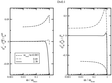
When , the CJ mode grows only slowly toward the horizon. It is thus possible to compute the other modes, see Footnote 3. With three independent modes at hand, we can compute the nine coefficients of the Bogoliubov transformation. Here, we present (for the first time in the literature) quantitative results concerning the production of left-moving particles, governed by . It is represented in the left panel of Fig. 19 as a function of for fixed to and for three values of , namely , and . We note that is, to a good approximation, linear in . Hence it does not go to zero when , in agreement with the fact that both and , and thus the coefficient in Eq. (23), remain well-defined above in the subluminal case.
In the right panel of Figure 19 the influence of the nonadiabatic parameter is investigated. As expected, the production of left-movers is more important when is higher. However the dependence on is weak and saturates when becomes high.
V.3.3 WH vs BH fluxes
Having access to the full Bogoliubov transformation of Eq. (23), we can also compute the difference between the fluxes emitted by WH and BH. From the algebraic treatment, we can assert (using the unitarity of Eq. (23)) that the difference of fluxes obeys
| (46) |
However, to actually compute this difference, a numerical treatment is required. The relative difference is represented in Fig. 20 for and and . This difference stays below . Moreover it decreases when increases, i.e. when going toward the robust regime, as one expected since it must vanish when the - mixing itself vanishes.
For the larger value of one can see that the relative difference changes sign. This can be understood from Eq. (46) and Fig. 19, where we have seen that is proportional to while , shown in the right plot in Fig. 20, is constant at low frequencies. Thus one always has at low enough frequencies. Notice also that contrary to the occupation numbers, and , neither of the ’s vanishes at , but they become equal, ensuring that at all frequencies Eq. (46) is satisfied.
Finally we notice that the relative difference does not diverge for , which implies that goes to zero near as quickly as .
V.4 Near region
To complete our study of the spectrum, we investigate the quick fall-off near . We find that, both for the energy flux and for , the fall-off presents a universal behavior (for the class of velocity profiles considered), independent of , and . Indeed we find that
| (47) |
where , and similarly for , with replaced by a different function of and , .
Fig. 21 shows and versus , near . is fixed to 50 and each curve corresponds to a different value of . Both quantities are linear when is close enough to , with a slope precisely equal to , independently of the value of . We verified that this behavior is also independent of . Finally we have also verified that the value of , which strongly affects the behavior of the spectrum near , as can be seen from Fig. 12, does not affect Eq. (47).

V.5 Integrated energy flux

In this section, we present the main features of the integrated energy flux obtained by integrating over the differential flux . It is computed as a Riemann sum and depends on , , and . The sum is computed from , where the asymptotic value of is reached to a good precision, until . The step in is , so that the relative variation between two successive points is small. Under these conditions, the Riemann sum gives a very good estimate of the integral.
The upper plot in Fig. 22 shows the integrated flux as a function of for several values of , and fixed to 2. Like and , the integrated flux converges rapidly to its standard value for , even though the flux density differs from the standard one for high frequencies. In other words, the nonlocal robustness criterium, that the integrated flux be close to standard, agrees with the local one defined in Sec. V.2. This is because the exponential tail of the standard contributes only marginally to the integral, so that the cut-off at in the modified flux does not cause noticeable differences in the integrated flux.
The lower plot of Fig. 22 shows that when increases, the amplitude of the oscillations in the integrated flux is more important, and they last until higher values of . This reflects the fact that the nonthermal part of yields a nonnegligible contribution to the integrated flux, and can be understood looking at Fig. 12 where the enhancement of the high frequency part of the spectrum through nonadiabatic effects was shown.
VI Results for superluminal dispersion
VI.1 General properties of the spectra
VI.1.1 Smallness of - mixing.

As can be seen from Eq. (30), is not exactly equal to . In the following we make the approximation , whose validity requires . To justify this, we first show that the inequality is indeed verified everywhere we can compute . is shown in Fig. 23 for different values of . At fixed , on the left plot, it strongly decreases when increases. For instance, it remains smaller than for . At fixed , on the right plot, it becomes monotonically decreasing only for high enough values of , but stays always smaller than for . These results strongly suggest that it must be even smaller in the region of the parameter space where it is inaccessible to our code. As we shall see in the next subsection, the important result is that it is always much smaller than both the modifications wrt the standard flux, and the relative difference between the super- and subluminal fluxes. The approximation thus induces only a negligible error.
VI.1.2 Comparison between super- and subluminal dispersion

In analogy with Eq. (38), we define the flux
| (48) |
To our surprise, we found that is extremely close to of Eq. (38) when working with the same background geometry (i.e. the same value of and ) and the same value of . This unexpected similarity shows once more that is the relevant parameter for characterizing the departure from the dispersionless case.
Although of Eq. (38) and belong to two different models, it does make sense to study their difference when one works with the same velocity profile , so as to have the same behavior in the dispersionless regime, and the same value of . (Under these conditions, the two values of cannot be exactly the same, but are close to one another.) In Fig. 24, the relative difference is represented versus for a fixed , and a series of increasing values of . The chosen values of correspond to respectively for subluminal dispersion, and slightly different values for superluminal dispersion, tuned to get the same . The relative differences are of about when , but are extremely small for and , except in a thin region near .
The right plot in Fig. 24 also represents the relative difference between and the standard energy flux. When the spectrum is not robust, as is the case for , the modifications with respect to the standard spectrum are much larger than the differences between the super- and subluminal spectra. In this sense, the modifications are controlled essentially by the value of , and seem to depend only marginally on the precise nature of the dispersion relation.
This point can be made more precise with the help of Fig. 25, where the same quantities as in Fig. 24 are represented, but this time with held fixed, equal to , and a varying . The values of corresponding to are respectively, for subluminal dispersion (and of course slightly different for superluminal dispersion). From the right plot in that figure, it is clear that for this fixed value of , large variations of cause only small variations in the corrections to the standard flux. In fact, as expected, the greater the scale separation between and , the more precise the statement that essentially only matters and not the precise nature of the dispersion relation. This is illustrated by the left plot, where we see that as decreases (and thus as increases to maintain fixed), the relative difference between and becomes smaller and smaller.
The smallness of the differences in the energy flux between sub- and superluminal dispersion teaches us several lessons. First, as soon as , the quantitative agreement, to a fraction of a percent, of the superluminal results with the subluminal ones (at least for frequencies not too close to ) means that the global properties for a given of the spectra for sub- and superluminal dispersion, such as the modified temperature, the running of the temperature, and the total energy flux, are the same to a very good approximation. Thus, we do not repeat in the case of superluminal dispersion the study performed in Sec. V.3 and Sec. V.5, since the results are qualitatively and quantitatively the same. Secondly, the robustness criterium and the range of robustness are the same for both types of dispersion. That is, the radiation is robust for in both cases.
VI.2 First corrections to HR in the robust regime

The above agreement between and suggests that the scaling of the leading corrections with respect to the standard spectrum are also similar for sub- and superluminal dispersion. This point is investigated in Fig. 26, where the logarithm of
| (49) |
is represented versus the logarithm of for several fixed values of and .
Like in the subluminal case, a “superrobust” regime is reached for . The slopes differ also slightly from the subluminal case. In the upper plot, we find for , , respectively. In the lower plot, the slopes are and for and respectively. The scaling in , at fixed , of the first corrections is still with a power close to in the superluminal case, while the scaling in at fixed is with a power between 2 and 3. It is also worth mentioning that is negative in the superrobust regime, as was . This is opposed to the first corrections to the inflationary spectra, that have different signs for sub- and superluminal dispersion (see [29]).
VI.3 Production of left-movers

Figure 27 shows the occupation number for superluminal dispersion for and the same values of as in Fig. 19. As in the subluminal case, it decreases when increases. It is proportional to for , but contrary to the subluminal case, it goes to zero when approaches . This is as expected since the negative frequency partners of these -quanta exist only for .
VI.4 Near region.
Finally, we have investigated the behavior of the fluxes near the maximum frequency. We find that both and decrease like near , as and did (see Eq. (47)).
VI.5 Comparison with Ref. [34]
In Ref. [34], when considering a time-dependent collapsing background metric, the authors reached the conclusion that Hawking radiation is no longer stationary when dealing with a quartic superluminal dispersion relation. We believe this conclusion is not due to the time-dependent character of the geometry, but is rather due to the use of a geometric optic approximation, in Eq. (4.14), in a regime where it is not valid, as indicated by the numerical results of [21]. However a detailed calculation of the fluxes remains to be done.
VII Conclusions
We have studied the properties of the fluxes emitted by acoustic black holes when taking into account the effects induced by sub- and superluminal dispersion relations. We focused on one dimensional stationary flows which possess two asymptotic regions. In this case, unlike what is found for gravitational black holes, the fluxes emitted on both sides of the horizon are well-defined observables.
At the theoretical level, we showed that the dimensionality of the space of asymptotically bounded stationary modes is three, and that this space is complete. This guarantees that the Bogoliubov transformation of Eq. (23) relating in and out modes is unitary. It reduces to a matrix only if left and right-moving modes completely decouple, which is a degenerate case, probably never found in condensed matter systems. We then showed that because of dispersion, there exists a critical frequency above which no radiation is emitted, and the transformation simplifies into Eq. (22). This frequency depends both on the UV scale characterizing the dispersion, and on the asymptotic properties of the background geometry. Because of the dispersion as well, the fluxes emitted by white holes are well-defined and regular. Moreover we established how they are related to those of the corresponding black hole, see Eq. (26) and Fig. 20.
We have computed numerically the fluxes in the case of quartic sub- and superluminal dispersion. The main result of our analysis is the following. The deviations wrt the standard dispersionless fluxes are highly degenerate along the lines of constant frequency , see Figs. 13 and 18, and, as a corollary, are essentially governed by .
Our second result concerns the characterization of the range of the robustness, i.e. the range of the parameters within which the deviations are small. We first found that for , there is a superrobust regime in which the leading deviations rapidly decrease as a power law in , where the power is equal to or depending on which parameter is held fixed, see Figs. 15 and 14. We also showed that for , the deviations are already smaller than a percent.
Our third important result concerns the absence of a significant running of the effective temperature, Eq. (42), even when leaving the robust regime. The low-frequency part of the fluxes, i.e. , is indeed well characterized by a common temperature that significantly differs, for , from the standard temperature but that hardly changes with , see the table after Eq. (42). This implies that the effective temperature is probably not related in a universal manner to the gradient of the flow velocity evaluated at some -dependent horizon, in agreement with the remarks made in [10].
Fourthly, we have also presented quantitative results concerning the production of -quanta in the domain . We found numerically that , is proportional to at low frequencies, see Figs. 19 and 27.
Finally we showed in Sec. VI that the deviations obtained using sub- and superluminal dispersion are unexpectedly similar when using theories having the same . This means that the deviations wrt to the standard fluxes obtained with each theory are much larger than the difference between these deviations, typically by a factor of more than , see Fig. 25. However these conclusions are probably related to the fact that our velocity profiles are symmetrical wrt the horizon, and possess two asymptotic regions. When considering profiles describing gravitational black holes, we expect that the deviations due to sub- and superluminal dispersion will differ more significantly. We also expect our results for subluminal dispersion to apply to gravitational black holes because the CJ modes essentially live in the outside region, as can be seen in Fig. 7.
Acknowledgements.
We would like to thank the organizers and the participants of the workshop “Towards the observation of Hawking radiation in condensed matter systems” (http://www.uv.es/workshopEHR/) held at IFIC in Valencia in February 2009, where the extension of this work to Bose-Einstein condensates was presented, for many interesting remarks. We are grateful to Jihad Mourad for discussions about the asymptotic bounded character of physical modes, and to Roberto Balbinot and Ted Jacobson for useful comments.Appendix A Role of decaying modes
In this appendix, our goals are, first, to show that in the black hole metric of Eq. (1), when using the dispersion relation Eq. (8) and for , the space of spatially bounded modes has dimension three, and secondly, to understand the physical roles of the decaying modes. In Sec. III.3, when considering homogeneous flows, we saw that both growing and decaying modes should be discarded from the field operator. When the flow is only asymptotically constant, as it is the case in Eq. (1), the symmetry between growing and decaying modes is broken because a mode that grows toward the horizon (we called this a ‘decaying’ mode) does not necessarily grow in the other asymptotic region.
In the asymptotic supersonic region of Eq. (1), the wave equation reduces to the same form as in an homogeneous flow with velocity . Thus, in this region, the general solution is a combination of all the exponential solutions that were present in the homogeneous case: four oscillatory solutions, decaying solutions, and growing solutions. This set defines the mathematically complete basis of modes (thereafter called the “left” basis), where labels the roots of Eq. (8) and stands for “left”, such that each has only one exponential component in the asymptotic supersonic region. When restricting ourselves to spatially bounded modes, the that correspond to growing components must be of course discarded. So one is left with independent modes bounded for , numbered by , .
In the subsonic asymptotic region, in general, these modes are not bounded because they are combinations of all exponential components, solutions of Eq. (8) with velocity . On that side, one has growing and decaying modes, and only two oscillatory modes. In order to get modes that are everywhere bounded, one must consider combinations of the form
| (50) |
The condition that the coefficients of the growing components in the subsonic region be all zero yields constraints on the coefficients . Therefore only three linearly independent bounded combinations exist. In other words, the dimensionality of the space of spatially bounded solutions is three for . This explains why only one extra-mode was added in Eq. (19). It is also important to note that the constraints in no way impose that the coefficients of the decaying modes be zero, and in fact the bounded modes, and in particular the ones constituting the in and out bases, generically contain decaying modes.
The physical role of these decaying modes is to ‘dress’ the in and out modes in the region where varies, in a way similar to the dressing of atoms by a local and nonpropagating polarization cloud when these are coupled to a radiation field [35]. Thus this dressing by decaying modes affects the properties of local observables (such as correlation functions) in the region where varies.
For completeness, a word on the construction of the in and out bases is in order. Just as we constructed the “left” basis, we can construct a “right” basis , from the asymptotic exponential solutions in the subsonic region. Looking at the space-time properties of wavepackets made out of the asymptotically oscillatory modes in both and , one can reclassify them into a group of three in modes and one of three out modes (still unbounded at this point). Each of these two groups mixes “left” and “right” modes. The dimensionality three of the space of bounded modes then ensures that we can find bounded combinations with only one in (respectively out) mode with a nonzero coefficient. These combinations, suitably normalized and possibly complex conjugated to get a positive norm mode, yield the in (resp. out) basis used in the text. Note also that since there are only two oscillatory solutions in the subsonic region, there exists one (and only one, up to an overall factor) bounded mode that is purely decaying in this region. This mode, correctly normalized, is the CJ mode, here generalized to arbitrary (polynomial) dispersion.
References
- [1] W. G. Unruh, Phys. Rev. Lett. 46, 1351 (1981).
- [2] T. Jacobson, Phys. Rev. D 44, 1731 (1991).
- [3] W. G. Unruh, Phys. Rev. D 51, 2827 (1995).
- [4] R. Brout, S. Massar, R. Parentani, and P. Spindel, Phys. Rev. D 52, 4559 (1995a), eprint hep-th/9506121.
- [5] S. Corley, Phys. Rev. D 57, 6280 (1998).
- [6] Y. Himemoto and T. Tanaka, Phys. Rev. D 61, 064004 (2000).
- [7] H. Saida and M.-A. Sakagami, Phys. Rev. D 61, 084023 (2000), eprint gr-qc/9905034.
- [8] W. G. Unruh and R. Schutzhold, Phys. Rev. D 71, 024028 (2005), eprint gr-qc/0408009.
- [9] R. Balbinot, A. Fabbri, S. Fagnocchi, and R. Parentani, Riv. Nuovo Cim. 28, 1 (2005), eprint gr-qc/0601079.
- [10] S. Corley and T. Jacobson, Phys. Rev. D 54, 1568 (1996), eprint hep-th/9601073.
- [11] W. G. Unruh, in proc. of the conf. “From Quantum to Emergent Gravity: Theory and Phenomenology”, PoS(QG-Ph)039 (2007).
- [12] C. Barcelo, S. Liberati, and M. Visser, Living Rev. Rel. 8, 12 (2005), eprint gr-qc/0505065.
- [13] T. Jacobson, S. Liberati, and D. Mattingly, Annals Phys. 321, 150 (2006), eprint astro-ph/0505267.
- [14] R. Parentani, Phys. Rev. D 63, 041503 (2001), eprint gr-qc/0009011.
- [15] R. Parentani, Int. J. Theor. Phys. 41, 2175 (2002a), eprint 0704.2563.
- [16] P. Horava, Phys. Rev. D 79, 084008 (2009), eprint 0901.3775.
- [17] H. Yoshino and V. S. Rychkov, Phys. Rev. D71, 104028 (2005), eprint hep-th/0503171.
- [18] J. Macher and R. Parentani (2009), eprint 0905.3634.
- [19] T. A. Jacobson and G. E. Volovik, Pisma Zh. Eksp. Teor. Fiz. 68, 833 (1998), eprint gr-qc/9811014.
- [20] R. Balbinot, A. Fabbri, S. Fagnocchi, A. Recati, and I. Carusotto, Phys. Rev. A 78, 021603(R) (2008), eprint 0711.4520.
- [21] I. Carusotto, S. Fagnocchi, A. Recati, R. Balbinot, and A. Fabbri, New J. Phys. 10, 103001 (2008), eprint 0803.0507.
- [22] S. Massar and R. Parentani, Phys. Rev. D 54, 7444 (1996).
- [23] R. Brout, S. Massar, R. Parentani, and P. Spindel, Phys. Rept. 260, 329 (1995b), eprint arXiv:0710.4345 [gr-qc].
- [24] T. G. Philbin et al., Science 319, 1367 (2008), eprint 0711.4796.
- [25] R. Parentani, Class. Quant. Grav. 25, 154015 (2008), eprint 0710.4664.
- [26] J. Adamek, D. Campo, J. C. Niemeyer, and R. Parentani, Phys. Rev. D 78, 103507 (2008), eprint 0806.4118.
- [27] R. Schutzhold and W. G. Unruh, Phys. Rev. D 78, 041504(R) (2008), eprint 0804.1686.
- [28] S. A. Fulling, Aspects of Quantum Field Theory in Curved Space-Time (Cambridge University Press, 1989).
- [29] J. Macher and R. Parentani, Phys. Rev. D 78, 043522 (2008), eprint 0804.1920.
- [30] T. Jacobson and D. Mattingly, Phys. Rev. D 61, 024017 (1999), eprint hep-th/9908099.
- [31] W. G. Unruh, Phys. Rev. D 14, 870 (1976).
- [32] R. Parentani, Int. J. Mod. Phys. A 17, 2721 (2002b), eprint gr-qc/0204079.
- [33] U. Leonhardt, T. Kiss, and P. Ohberg (2002), eprint gr-qc/0211069.
- [34] C. Barcelo, L. J. Garay, and G. Jannes, Phys. Rev. D 79, 024016 (2009).
- [35] S. Massar, R. Parentani, and R. Brout, Class. Quant. Grav. 10, 385 (1993).