Adaptive Mesh Approach for Predicting Algorithm Behavior
with Application to Visibility Culling in Computer Graphics

Matthias Fischer Affiliation: Heinz Nixdorf Institute and Department of Computer Science, University of Paderborn, GERMANY Claudius Jähn ^†^†thanks: Supported by DFG grants Me 872/12-1 within SPP 1307 and Research Training Group GK-693 of the Paderborn Institute for Scientific Computation (PaSCo), contact author Affiliation: Heinz Nixdorf Institute and Department of Computer Science, University of Paderborn, GERMANY Martin Ziegler ^†^†thanks: Supported by Zi 1009/2-1 Affiliation: Institute for Theoretical Physics, Vienna University of Technology, AUSTRIA

Abstract

We propose a concise approximate description, and a method for efficiently obtaining this description, via adaptive random sampling of the performance (running time, memory consumption, or any other profileable numerical quantity) of a given algorithm on some low-dimensional rectangular grid of inputs. The formal correctness is proven under reasonable assumptions on the algorithm under consideration; and the approach’s practical benefit is demonstrated by predicting for which observer positions and viewing directions an occlusion culling algorithm yields a net performance benefit or loss compared to a simple brute force renderer.

1 Introduction

Although it is possible to give bounds for different aspects of many algorithms’ runtime behaviors (like for running time or memory consumption) by formal analysis, the input can heavily influence the actual behavior (e.g. algorithms for real-time rendering of virtual 3d-scenes). To evaluate algorithms for practical applications, in which the input (or the characteristics of the input) is known, a more detailed estimation of the algorithm’s behavior s necessary in order to

•

select the appropriate algorithm for the given setting (hardware, application and input).
•

find suitable parameters to adapt the selected algorithm to the setting.
•

identify bottlenecks and starting points for further improvements of the algorithm.

If the number of possible inputs is sufficiently small, it may be possible to evaluate the observed property of the algorithm (e.g. the running time) for every input and use this as basis for the evaluation. But in most cases the input space is too big (e.g. all possible positions inside a virtual scene), so that only a few samples can be evaluated experimentally. For a simple uniform sampling approach, it is difficult to capture the structures the input may exhibit. Another common way in computer graphics is e.g. to select a camera path covering all relevant inputs manually.

But if small changes in the input mostly lead to small changes in the behavior of the algorithm only, we can apply our adaptive sampling method. Thereby the input space is subdivided into regions, in which the algorithm behaves similarly. This subdivision can then represent an easy-to-handle model of the algorithm.

In the following, we

i)

present the method that creates this subdivision of the input.
ii)

prove that, if the function, which describes the behavior of the algorithm is Lipschitz-continuous, it can be approximated by this method.
iii)

evaluate the method in the domain of real-time 3d rendering, in which we can make use of the distinct local coherence of many rendering algorithms.

The goal of our approach is to preprocess a given algorithm via blackbox queries at certain inputs, in order to quickly and approximately predict its behavior on other inputs. The data structure constructed during preprocessing is a hierarchical subdivision described in Section 2 and gives a kind of global picture of the algorithm under consideration with many applications to Algorithm Engineering (Section 2.1). The success of our approach is both proven formally in Section 3 (under reasonable analytical assumptions) and^§^§ § Note that we do not claim Occlusion Culling to behave Lipschitz-continuously, but rather consider ii) and iii) as two classes of scenarios that benefit from i) demonstrated empirically on the Occlusion Culling problem in Computer graphics: see Sections 4, 5, 6 and 7.

2 Randomized Adaptive Hierarchical Subdivision

Consider a $d$ -dimensional cuboid $C=[a_{1},b_{1}]\times[a_{2},b_{2}]\cdots[a_{d},b_{d}]\subseteq\mathbb{R}^{d}$ . We want to approximate an unknown function $f:C\to\mathbb{R}$ , accessable through blackbox queries for its values $f(\vec{x})$ at given arguments $\vec{x}$ , by a piece-constant function consisting of ‘few and simple’ pieces.

Algorithm 2.1

Fix dimension $d\in\mathbb{N}$ , sample size $k$ , so-called splitting threshold $s>0$ , and the unknown $f:C\subseteq\mathbb{R}^{d}\to\mathbb{R}$ .

•

Sample $k$ arguments $\vec{x}_{1},\ldots,\vec{x}_{k}\in C$ independently uniformly at random.
•

Query values $y_{i}:=f(\vec{x}_{i})$ , $1\leq i\leq k$ .
•

If $|y_{i}-y_{j}|\leq s$ holds for all $1\leq i,j\leq k$ ,
replace $f$ on $C$ by the constant function $g\equiv z:=\operatorname{avrg}(y_{1},\ldots,y_{k})$ .
•

Otherwise cut $C$ into $2^{d}$ subcuboids of equal size
and recurse to (the restrictions of $f$ to) each of them.

The underlying idea is simple: If values $f(\vec{x}_{i})$ and $f(\vec{x}_{j})$ deviate too much, then the cuboid cannot be accurately described by a constant function on entire $C$ .

Refer to caption — Figure 1: Example piecewise constant approximation $g$ of a function $f:[a_{1},b_{1}]\times[a_{2},b_{2}]\to\mathbb{R}$ as output by Algorithm 2.1: Shades of gray indicate the values of $g$ .

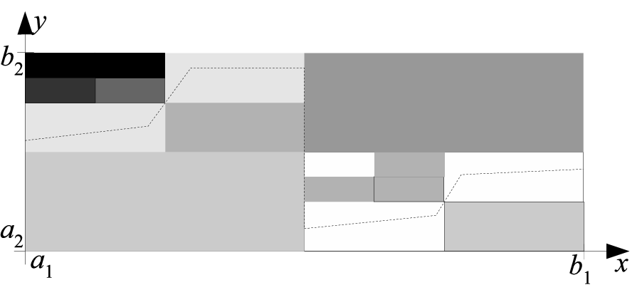
Note that the recursive process of Algorithm 2.1 yields a piecewise constant function $g$ , in which the locally constant parts constitute a hierarchical subdivision known in 2D as quadtree (indicated in Figure 1) and in 3D as octree. In particular, this $g$ naturally comes with a very practical and efficient representation as a data structure: a hierarchical subdivision. That is, Algorithm 2.1 can be considered as preprocessing $f$ for the following interpolation:

Algorithm 2.2

Fix a $d$ -dimensional octree $T$ over $C$ as produced by Algorithm 2.1.
Given $\vec{x}\in C$ , iteratively

•

determine which of the $2^{d}$ subcuboids $C^{\prime}$ of $C$ this input $\vec{x}$ lies in;
•

proceed to this $C^{\prime}$ (i.e. to the corresponding subtree of $T$ )
•

unless $C$ is already a leaf of $T$ .
•

In the latter case, return the constant value $z$ of $g$ on $C$ .

Because of the exponential term $2^{d}$ , this approach can be efficient only for small values of $d$ . (In Section 4 we will apply it for $d=2\tfrac{1}{2}$ : two spatial dimensions and a discrete directional one.) The piecewise constant function $g$ , output by Algorithm 2.1 (and thus also the extrapolated values produced by Algorithm 2.2) can of course not be expected to approximate the given $f$ in general. But Section 3 asserts that it does so for Lipschitz-continuous $f$ and sufficiently large sample sizes.

2.1 Applications of the Hierarchical Subdivision to Algorithm Engineering

Consider some algorithm $A$ operating on (integral or continuous) inputs $\vec{x}$ from the cuboid $C$ . Let $f(\vec{x})$ denote the value at input $\vec{x}$ of some profileable quantitative property of $A$ . This may for instance be running time, memory consumption, number of instructions etc. (Section 4 will for example consider the number of occlusion queries.) Then Algorithm 2.1 produces a hierarchical subdivision of $C$ and piecewise constant approximation $g$ to $f$ from profiled values $f(\vec{x})$ at ‘few’ adaptively sampled inputs $\vec{x}$ ; and Algorithm 2.2 uses this data structure to approximately predict the value $f(\vec{x})$ (i.e. the quantitative property of algorithm $A$ ) on other inputs $\vec{x}\in C$ .

Now this approach cannot be expected to succeed all the time and for every $A$ . On the other hand many practical algorithms (in particular those operating on continuous, e.g. floating point data) do exhibit some sort of continuity—if not strictly, then in the mollified sense of local averages. In fact such kind of benignity is analogous to the temporal and spatial locality hypotheses which both, caching (data) and instruction prefetch / branch prediction (control) techniques successfully do rely on. And if Algorithm 2.1 does yield a good approximation of the behavior of $A$ , this can be employed in various ways:

Realistic Rating and Comparison of Algorithms: A picture as in Figure 1 summarizes the behavior of the underlying algorithm $A$ rather nicely. One can easily read off regions of inputs, in which $A$ takes long (dark) or little time (bright). A similar one for another algorithm $B$ permits to decide for which regions $A$ may succeed over $B$ and by how much.

Average-Case Performance Estimation for Generic Input Distributions: Worst-case running times often suffer from few, but practically rare ‘bad’ inputs. An average case statement is restricted to one specific input distribution and may be useless to another. The hierarchical decomposition produced by Algorithm 2.1 on the other hand allows to estimate average case properties for many distributions on input space. In fact the octree needs to be determined only once: a distribution then amounts to assigning weights to the sub(sub)cuboids and the induced average case property to a mere (re-)calculation of their weighted average. The worst-case can be read off as well.

Empirical Algorithm Evaluation on Generic Hardware: Algorithm 2.1 can be applied to the same $A$ in order to determine various profileable quantities $f_{i}$ separately, for instance to count how often it performs operation $a_{1}$ , , $a_{2}$ , etc. . Now suppose that on some specific hardware $H$ , $a_{i}$ takes time $t_{i}$ : Then the total time used by $A$ can be estimated as $\sum_{i}f_{i}\cdot t_{i}$ (for sequential execution; $\max_{i}f_{i}\cdot t_{i}$ for parallel, and similarly for mixed execution) by mere calculation, i.e. without actually having to execute $A$ on $H$ .

Parameter Optimization: Suppose some algorithm $A$ has $d$ input dimensions and $k$ parameters. A common topic in algorithm engineering is how to choose these parameters (in dependence of the specific inputs and hardware) in order to to gain optimum performance. For example, many tree-based algorithms behave much better when collapsing all ‘small’ subtrees of size below a certain threshold into simple arrays. This threshold value is the parameter to be optimized. Again, this is a problem which the data structure generated by Algorithm 2.1 can help solving. In Figure 1 for instance, $y$ as a parameter would be chosen in dependence of input $x$ as indicated by the dashed line because that yields an overall performance below the 10% grey level.

Automatic Adaption to Computational Environments combines parameter optimization with the performance prediction from generic to specific hardware.

2.2 Applications of the Subdivision to the Rendering of Virtual Scenes

In this section, we transfer the proposed applications to Algorithm Engineering in the field of real-time rendering of 3d-scenes. We give an introduction to the problems and the algorithms we use for the examples and give an overview over the covered applications of the subdivision method in this domain.

Our field of interest is the occlusion culling problem in computer graphics: Interactive display of highly complex scenes like landscapes with extensive vegetation, large city models, or highly detailed datasets in scientific visualization are a major challenge for rendering algorithms. Although the capabilities of computer graphics hardware have dramatically increased in the past decades, the handling of scene complexity is still one of the most fundamental problems in computer graphics. A large number of approaches have been proposed to handle high scene complexity in interactive applications [MH99, LRC+03]. In this paper we focus on occlusion culling: trying to avoid bothering with rendering parts of the scene which are not visible to the observer anyway. A multitude of algorithms has been suggested and is being employed for this purpose [CCSD03, Dur00]. This raises even more questions of whether and under which circumstances, one algorithm may be superior to the other.

We apply and evaluate the approach of Section 2.1 as a means to solve this problem. Specifically we consider two fundamentally different rendering algorithms: the brute-force way of sending all triangles of the scene to the graphics pipeline and a recent one [BWPP04]. The latter algorithm uses a feature of modern graphic adapters, which allows counting an object’s number of pixels , which pass the depth test of the rendering pipeline and are therefore not occluded by a previous object. In order to make use of this feature, the virtual scene is organized in a tree that represents a bounding volume hierarchy, in which the axis aligned bounding box of a node encloses the boxes and geometrical objects of all children (here we use an octree). The rendering algorithm traverses the nodes of the tree (the nodes are thereby ordered front-to-back from the observer’s position) and before a node is rendered, it’s bounding box is tested for if it does contribute at least one pixel to the frame buffer. If it’s bounding box is not fully occluded, all associated objects are rendered and the traversal continues with the child nodes. If the box is hidden, the corresponding subtree is skipped for this frame since all children can only lie inside this box, as well and are completely occluded. As the visibility test itself needs to pass the rendering pipeline, it takes some time for it’s result to be available. To hide this delay, the algorithm continues with the rendering of the scene and updates the visibility information when the result arrives. This can result in the futile rendering of some hidden nodes, but is still faster than locked waiting.

In the evaluation we apply the presented applications (Section 2.1) to these rendering algorithms in the field of computer graphics.

1.

We use hierarchical subdivisions to globally compare the algorithms according to their running time and evaluate the occlusion culling efficiency (in Section 4).
2.

We use the average values of subdivisions according to running time in order to identify the optimal value for the maximum octree-depth in the example setting (In Section 5).
3.

Section 6 gives an overview on how the running time can be predicted with subdivisions according to the components of a cost function for generic hardware.
4.

In Section 7 we present how subdivisions in this area can be extended to include additional information about the viewing direction in order to online select the best rendering algorithm depending on the position and the viewing direction.

2.3 Related Work

There is a vast literature on algorithmic methods for adaptively and hierarchically approximating an unknown function $f$ piecewise by simpler ones.

i) Numerical treatment of a function $f$ on some smooth manifold $\mathcal{M}$ (e.g. the solution to a partial differential equation using the Finite Elements Method FEM) generally proceeds by first triangulating $\mathcal{M}$ and replacing $f$ on each such triangle by a linear function. For reasons of accuracy, the thus considered mesh on $\mathcal{M}$ is usually desired to be finer on regions of high curvature (corresponding to large variations of $f$ ) and coarse on ‘flat’ parts of $\mathcal{M}$ ; cf. e.g. [PLW05].

ii) Also well-known are various methods of approximately ‘learning’ an unknown function $f$ by querying its values $f(\vec{x})$ on appropriately chosen arguments $\vec{x}_{i}$ . This is in fact the essence of information-based complexity [TWW88], e.g. for numerically integrating $f$ . Again, the evaluation points are preferably chosen adaptively: more densely if, and where, $f$ exhibits strong variations.

A synthesis of i) and ii) concerning Lipschitz-continuous functions (cf. Section 3 below), the work [BDK08] is concerned with 1D integration; and [Coop95, Beli06] focus on deterministic uniform approximation of $f$ by piecewise linear functions. We point out that i+ii) can also be considered as lossy function compression problems: replacing a (possibly complicated) $f$ by some simple $g$ resembling $f$ . ‘Simple’, here means, piecewise constant or linear; for other classes of simple functions (like, e.g., sines and cosines) one arrives at wavelets and Fourier compression with famous applications such as mp3 and jpeg.

The main idea of the present work is to apply these methods to a seemingly unrelated but notorious problem in Algorithm Engineering in general and especially in computer graphics:

iii) Predicting the behavior of an algorithm, e.g., runtime. This has been a major topic particularly in parallel and distributed computing—compare e.g. [FRW96, BMW02, BGLR04]—and to computer graphics [FS93, WiWo03].

iv) Evaluating the efficiency (runtime, frames) of a rendering algorithm. Typically, the target function is measured along a chosen camera path [FS93] or with an increasing scene complexity (number of polygons) [CDL+96] or for some fixed chosen viewing points [PZvBG00].

v) To maintain an adaptive rendering algorithm. This has been applied to real-time rendering systems to adaptively adjust image quality in oder to maintain a uniform, user-specified target frame rate [FS93].

3 Asymptotic Analysis and Correctness of the Approach

As already mentioned, Algorithms 2.1 and 2.2 cannot be expected to succeed on an arbitrary unknown function. We now prove that they do approximate such $f:C\to\mathbb{R}$ with high probability, if $f$ is Lipschitz-continuous, provided that the sample size is large enough. More precisely Theorem 3.1 asserts successful approximation up to given absolute error

•

uniformly for sample size roughly proportional to the volume of $C$
•

in the least squares-sense for sample size roughly proportional to the diameter of $C$ .

Both are shown asymptotically best possible.

3.1 Reminder and Properties of Lipschitz-continuous Functions

For $c>0$ , a classical notion in calculus calls a function $f:\operatorname{dom}(f)\subseteq\mathbb{R}^{d}\to\mathbb{R}$ $c$ -Lipschitz if $|f(\vec{x})-f(\vec{y})|\leq c\cdot\|\vec{x}-\vec{y}\|$ holds for all $\vec{x},\vec{y}\in\operatorname{dom}(f)$ . For instance any differentiable $f$ with derivative bound $\|f^{\prime}(\vec{x})\|^{\prime}\leq c$ is $c$ -Lipschitz. Here $(\|\,\cdot\,\|,\|\,\cdot\,\|^{\prime})$ denotes a dual pair of norms, which is satisfying the Hölder Inequality $|\langle\vec{x},\vec{y}\rangle|\leq\|\vec{x}\|\cdot\|\vec{y}\|^{\prime}$ for all $\vec{x},\vec{y}\in\mathbb{R}^{d}$ ; e.g. Euclidean norms, or $\|\vec{x}\|=(\sum_{i}|x_{i}|^{p})^{1/p}$ and $\|\vec{y}\|^{\prime}=(\sum_{i}|y_{i}|^{q})^{1/q}$ with $1=1/p+1/q$ .

We also remark that any continuous function on $C$ is $c$ -Lipschitz for some (but possibly very large) $c$ , because $C$ is compact.

Lemma 1

Let $\mu$ denote a probability measure on $C=[a_{1},b_{1}]\times[a_{2},b_{2}]\cdots[a_{d},b_{d}]\subseteq\mathbb{R}^{d}$ , i.e. with $1=\mu(C)=\int_{C}1\,d\mu$ . Moreover write $\operatorname{diam}(C):=\sup\{\|\vec{x}-\vec{y}\|:\vec{x},\vec{y}\in C\}$ and $B(\vec{x},r):=\{\vec{y}\in C:\|\vec{x}-\vec{y}\|\leq r\}$ . Finally consider a $c$ -Lipschitz function $f:C\to\mathbb{R}$ .

a)

For $s>0$ and $\vec{y}\in C$ , it holds: $\displaystyle\big\{\vec{x}\in C:|f(\vec{x})-f(\vec{y})|\leq s\big\}\supseteq B(\vec{y},s/c)$ .
b)

Let $\lambda:=\min_{\vec{y}\in C}\mu\big(B(\vec{y},s/c)\big)$ and suppose $\sup_{C}f-\inf_{C}f>4s$ . Then $k:=1/\lambda$ points $\vec{x}$ , sampled from $C$ according to the distribution $\mu$ , contain with constant probability some $\vec{x}_{i},\vec{x}_{j}$ such that $|f(\vec{x}_{i})-f(\vec{x}_{j})|>s$ .

For any $\vec{y}\in C$ and $s>0$ and measurable $C^{\prime}\subseteq C$ , it holds

\int\nolimits_{C^{\prime}}|f(\vec{x})-f(\vec{y})|\>d\mu(\vec{x})\quad\leq\quad s\;\;+\;\;c\cdot\operatorname{diam}(C)\cdot\mu\{\vec{x}\in C^{\prime}:|f(\vec{x})-f(\vec{y})|>s\}\kern 5.0pt.

Let $\mu$ either be the normalized Lebesgues measure on $C$ or the normalized integer counting measure on $C$ , i.e. $\mu(C^{\prime})=\operatorname{Card}(C^{\prime}\cap\mathbb{Z}^{d})/\operatorname{Card}(C\cap\mathbb{Z}^{d})$ . Then it holds

\int\nolimits_{C}f(\vec{x})^{2}\,d\mu(\vec{x})\quad\leq\quad\mathcal{O}(\sqrt{\operatorname{diam}C})\cdot\Big(\int\nolimits_{C}|f(\vec{x})|\,d\mu(\vec{x})\Big)^{2}\quad+\quad\mathcal{O}(c^{2})\kern 5.0pt.

Concerning d) remember that, without Lipschitz-condition, $\int_{0}^{1}f(x)^{2}\,dx$ in general cannot be bounded in terms of $\int_{0}^{1}|f(x)|\,dx$ : consider $x\mapsto 1/\sqrt{x}$ . Also, $\sqrt{\operatorname{diam}C}$ is asymptotically best possible in 1D, since the 1-Lipschitz function on $[0,n]$ depicted in Figure 2b) has, for the normalized Lebesgues measure $d\mu=dx/n$ , $\int|f|\,d\mu=\theta(1)$ and $\int|f|^{2}\,d\mu=\Theta(n^{1/2})$ . Similarly, the sample size of Lemma 1b) is asymptotically best possible for the function depicted in Figure 2a).

Proof (Lemma 1)

a) Since $f$ is $c$ -Lipschitz, $\|\vec{x}-\vec{y}\|\leq s/c$ implies $|f(\vec{x})-f(\vec{y})|\leq s$ .

b)

Let $z:=(\sup f+\inf f)/2$ , $\vec{y}_{+},\vec{y}_{-}\in C$ with $f(\vec{y}_{+})=\sup f$ and $f(\vec{y}_{-})=\inf f$ , exploiting that $f$ is continuous on compact $C$ . Then $C_{+}:=\{\vec{x}\in C:f(\vec{x})>z+s\}\supseteq\{\vec{x}:|f(\vec{x})-f(\vec{y}_{+})|\leq s\}$ and $C_{-}:=\{\vec{x}:f(\vec{x})<z-s\}$ both have $\mu(C_{+}),\mu(C_{-})\geq\lambda$ by a). Hence $1/\lambda$ points $\vec{x}$ sampled from $C$ have probability $1-(1-\lambda)^{1/\lambda}\geq 1-1/e$ of hitting some $\vec{x}_{i}\in C_{+}$ ; similarly for hitting some $\vec{x}_{j}\in C_{-}$ : and since $C_{+}\cap C_{-}=\emptyset$ are independent, a constant probability $\geq(1-1/e)^{2}$ for both. These satisfy $|f(\vec{x}_{i})-f(\vec{x}_{j})|>s$ .

Observe that probability measure satisfies $\mu\{\vec{x}\in C^{\prime}:|f(\vec{x})-f(\vec{y})|\leq s\}\leq\mu(C)=1$ and

\int\limits_{C^{\prime}}|f(\vec{x})-f(\vec{y})|\>d\mu(\vec{x})\quad\leq\quad\int\limits_{\makebox[31.88898pt][l]{$\scriptscriptstyle\vec{x}\in C^{\prime}:|f(\vec{x})-f(\vec{y})|\leq s$}}s\,d\mu(\vec{x})\quad+\quad\int\limits_{\makebox[31.88898pt][l]{$\scriptscriptstyle\vec{x}\in C^{\prime}:|f(\vec{x})-f(\vec{y})|>s$}}c\cdot\|\vec{x}-\vec{y}\|\,d\mu(\vec{x})

W.l.o.g. suppose $f:[0,N)\to\mathbb{R}$ is nonnegative and $1$ -Lipschitz; otherwise consider $|f|/c$ . Consider the real sequence $\vec{y}$ defined by $y_{0}:=\max\{1,f(0)\}$ , $y_{1}:=\max\{1,f(y_{0})\}$ , $y_{2}:=\max\{1,f(y_{0}+y_{1})\}$ , $y_{i+1}:=\max\{1,f(y_{0}+y_{1}+\cdots+y_{i})\}$ . Since $y_{i}\geq 1$ , it holds $\sum_{i\leq n}y_{i}\geq N$ for some $n\leq N$ ; truncate $y_{n}$ such that $\sum_{i<n}<\sum_{i\leq n}y_{i}=N$ . Moreover let $I\subseteq\{1,\ldots,n\}$ denote the set of those $i$ with $y_{i}>1$ and in particular $y_{i}=f(\sum_{j<i}y_{j})$ . Because of the Lipschitz condition, it holds

y_{i}-x\leq f(\sum_{j<i}y_{j}+x)\overset{(*)}{\leq}y_{i}+x\quad\text{ for all $0\leq x<y_{i}$ and all $i\in I$; \quad(*) even for all $i$.}

Thus, $\int_{0}^{y_{i}}f(\sum_{j<i}y_{j}+x)\,dx\geq y_{i}^{2}/2$ for $i\in I$ and $\int_{0}^{y_{i}}f(\sum_{j<i}y_{j}+x)^{2}\,dx\leq y_{i}^{3}\cdot 7/3$ for all $i$ ; in particular $\leq 7/3$ for $i\not\in I$ . Therefore,

1/N\cdot\int_{0}^{N}|f|\,dx\;\;=\;\;1/N\cdot\sum\limits_{i}\int_{\sum_{j<i}y_{j}}^{\sum_{j\leq i}y_{j}}|f|\,dx\;\;\geq\;\;\tfrac{1}{2}\cdot\sum\limits_{i\in I}y_{i}^{2}/\sum\limits_{i\in I}y_{i}\;\;=\;\;\tfrac{1}{2}\|\vec{y}\|_{2}^{2}/\|\vec{y}\|_{1}

with the abbreviation $\vec{y}:=(y_{i})_{{}_{i\in I}}$ . Similarly,

	$\displaystyle 1/N\cdot\int_{0}^{N}\|f\|^{2}\,dx$	$\displaystyle\leq$	$\displaystyle 1/N\cdot\sum_{i\in I}\int_{\sum_{j<i}y_{j}}^{\sum_{j\leq i}y_{j}}\|f\|^{2}\,dx\;+\;1/N\cdot\sum_{i\not\in I}7/3$
		$\displaystyle\leq$	$\displaystyle\tfrac{7}{3}\\|\vec{y}\\|_{3}^{3}/\\|\vec{y}\\|_{1}\;+\;7/3\;\overset{(**)}{\;\leq\;}\;\tfrac{7}{3}\sqrt{N}\cdot\\|\vec{y}\\|_{2}^{4}/\\|\vec{y}\\|_{1}^{2}\;+\;7/3$

where at (**) we have employed Jensen’s Inequality $\|\vec{y}\|_{3}\leq\|\vec{y}\|_{2}$ as well as the bound $\|(y_{1},\ldots,y_{k})\|_{1}\leq\sqrt{k}\|(y_{1},\ldots,y_{k})\|_{2}$ . ∎

3.2 Sample Sizes for Uniform and for Residual Sum-of-Squares Approximation

First note that Algorithm 2.1 terminates for $c$ -Lipschitz continuous functions $f:C\to\mathbb{R}$ : If $c\cdot\operatorname{diam}(C)\leq s$ holds, then line 3 strikes; and this happens latest at a recursion depth of order $\log\big(c\cdot\operatorname{diam}(C)/s)$ .

Theorem 3.1

Let $\mu$ denote either the normalized Lebesgues measure or the normalized integer counting measure on $C$ .

i)

Consider $k^{\prime}:=\operatorname{vol}(C)\cdot c^{d}/s^{d}$ with $\operatorname{vol}(\mathop{\times}_{i}[a_{i},b_{i}]):=\prod_{i=1}^{d}(b_{i}-a_{i})$ . Then Algorithm 2.1 with $k:=k^{\prime}\cdot\log^{2}(k^{\prime})$ produces $g$ such that $\|f-g\|_{\infty}\leq 4s$ holds with high probability;
ii)

Suppose $s>c$ and consider $k^{\prime}:=\sqrt{\operatorname{diam}C}+c\cdot\operatorname{diam}(C)/s$ . Then Algorithm 2.1 with $k:=k^{\prime}\cdot\log^{2}(k^{\prime})$ produces $g$ such that $\|f-g\|_{2}\leq 4s$ holds with high probability.

We remark that the uniform approximation in i) is based on samples of size $k$ , essentially linear in $\operatorname{vol}(C)$ ; whereas the least squares approximation in ii) takes samples of size proportional to the diameter—which is asymptotically smaller in dimensions $d\geq 2$ . Note that a sample size of order $\operatorname{diam}^{1-\epsilon}/s$ is necessary in the worst case:

Example 3.2

Fix $\epsilon>0$ and generalize the function in Figure 2b) to 1-Lipschitz $f_{\epsilon}:[0,n]\to[0,n]$ defined by

f(x):=n^{1-2\epsilon}-x\quad\text{for }x\leq m:=n^{1-2\epsilon}+a\cdot n^{1-4\epsilon},\qquad f(x):=-a\cdot n^{1-4\epsilon}\quad\text{for }x\geq m\kern 5.0pt.

Then $\int_{0}^{n^{1-2\epsilon}}f(x)\,dx=n^{2-4\epsilon}/2$ , $\int_{n^{1-2\epsilon}}^{m}f(x)\,dx=-a^{2}\cdot n^{2-8\epsilon}/2$ , and $\int_{m}^{1}f(x)\,dx=-(n-m)\cdot a\cdot n^{1-4\epsilon}$ ; hence the mean is $\int_{0}^{n}f(x)=0$ for some appropriate $a=\tfrac{1}{2}+o(1)$ . Moreover $\int_{0}^{n^{1-2\epsilon}}|f(x)|^{2}\,dx=n^{3-6\epsilon}/3$ and $\int_{n^{1-2\epsilon}}^{n}|f(x)|^{2}\,dx=\Theta(n^{3-8\epsilon})$ , hence the variance is $\sigma=\sqrt{1/n\cdot\int_{0}^{n}|f|^{2}\,dx}=\Theta(n^{1-3\epsilon})$ . Now consider $s:=\sigma/2$ and observe that, in order to approximate $f$ up to error $s$ , any algorithm has to distinguish it from some other function $f^{\prime}:[0,n]\to[\pm s/2]$ and therefore needs to detect $x_{i},x_{j}$ with $f(x_{i})-f(x_{j})\geq s$ . Since $f(x)\in[-\Theta(n^{1-4\epsilon}),0]\subseteq[-s/2,+s/2]$ for $x\geq n^{1-2\epsilon}$ and $n$ sufficiently large, such an algorithm must in particular (yet does not suffice to) find at least one $x_{i}\leq n^{1-2\epsilon}$ : which for one single sample happens with probability $n^{1-2\epsilon}/n=\Theta(s/n^{1-\epsilon})$ where $n=\operatorname{diam}[0,n]$ . ∎

Proof (Theorem 3.1)

i)

First observe that in case $\sup_{C}f-\inf_{C}f\leq 4s$ , any sampled $\vec{x}\in C$ will yield $g:\equiv f(\vec{x})$ with $\|f-g\|_{\infty}\leq 4s$ ; whereas in case $\sup_{C}f-\inf_{C}f>4s$ , Algorithm 2.1 has a high probability of cutting $C$ into smaller parts: this follows from Lemma 1b) by probability amplification due to the logarithmic oversampling. Since the algorithm has logarithmic recursion depth with sub-subcuboids of exponentially fast decreasing size before arriving at constant volume, the $\log^{2}$ -factor maintains the high success probability throughout.

ii)

The mean $z:=\int_{C}f(\vec{x})\,d\mu(\vec{x})$ is well-known to minimize $\int_{C}|f(\vec{x})-z|^{2}\,d\mu(\vec{x})=\|f-z\|_{2}^{2}$ (or, equivalently, $\|f-z\|_{2}$ ). Observe that $C_{+}:=\{\vec{x}\in C:f(\vec{x})\geq z\}$ and $C_{-}:=\{\vec{x}\in C:f(\vec{x})<z\}$ satisfy $1=\mu(C_{-})+\mu(C_{+})$ and

	$\displaystyle 0\;=\;\int_{C}\big(f(\vec{x})-z\big)\,d\mu(\vec{x})$	$\displaystyle\;\;=\;$	$\displaystyle\int_{C_{+}}\|f(\vec{x})-z\|\,d\mu(\vec{x})\;\;-\;\;\int_{C_{-}}\|f(\vec{x})-z\|\,d\mu(\vec{x})\kern 5.0pt,$
	$\displaystyle\int_{C}\|f(\vec{x})-z\|\,d\mu(\vec{x})$	$\displaystyle\;\;=\;$	$\displaystyle\int_{C_{+}}\|f(\vec{x})-z\|\,d\mu(\vec{x})\;\;+\;\;\int_{C_{-}}\|f(\vec{x})-z\|\,d\mu(\vec{x})\kern 5.0pt;$

hence $\int_{C_{\pm}}|f(\vec{x})-z|\,d\mu(\vec{x})=\tfrac{1}{2}\int_{C}|f(\vec{x})-z|\,d\mu(\vec{x})$ . W.l.o.g. $\mu(C_{+})\geq 1/2$ .
Now first suppose $s>\tfrac{1}{4}\|f-z\|_{2}/\sqrt[4]{\operatorname{diam}C}$ . Recall Bernstein’s Inequality

\operatorname{Pr}\Big[\;\big|\sum\nolimits_{i=1}^{k}X_{i}/k-z\big|\>>\>s\;\Big]\quad\leq\quad 2\cdot\exp\Big(-\frac{ks^{2}}{2\sigma^{2}+(b-a)\cdot s}\Big)

for $k$ independent random variables $X_{i}\in[a,b]$ with mean $z$ and variance $\sigma=\|f-z\|_{2}$ . Here $X_{i}:=f(\vec{x}_{i})\in[z\pm c\cdot\operatorname{diam}C]$ because of the Lipschitz condition. Hence $k\geq 32\cdot\sqrt{\operatorname{diam}C}+c\cdot\operatorname{diam}(C)/s$ samples suffice for the sample average in line 4 of Algorithm 2.1 to be closer than $s$ to the true mean $z$ with constant probability.
This time suppose $s>\tfrac{1}{4}\|f-z\|_{2}/\sqrt[4]{\operatorname{diam}C}$ . Then, by Lemma 1c),

\mu(\{\vec{x}\in C:f(\vec{x})<z-s\})\quad=\quad\mu(\{\vec{x}\in C_{-}:|f(\vec{x})-z|>s\})\quad\geq\\ \quad\geq\quad\Big(\int\nolimits_{C_{-}}|f(\vec{x})-z|\,d\vec{x}\;-\;s\Big)/(c\cdot\operatorname{diam}C)\quad=\quad\frac{\|f-z\|_{1}/2-s}{c\cdot\operatorname{diam}C}

where, according to Lemma 1d) and in the big-Oh sense,

\|f-z\|_{1}\;\geq\;\sqrt{\|f-z\|^{2}_{2}-c^{2}}/\sqrt[4]{\operatorname{diam}C}\;\geq\;(\|f-z\|_{2}-c)/\sqrt[4]{\operatorname{diam}C}\;\geq\;4s-c/\sqrt[4]{\operatorname{diam}C}\kern 5.0pt,

hence $\mu(\{\vec{x}\in C:f(\vec{x})<z-s\})\geq(3s-c)/(c\cdot\operatorname{diam}C)$ . So a sample of size $k\geq(c\cdot\operatorname{diam}C)/(3s-c)$ has constant probability for Algorithm 2.1 to find some $\vec{x}_{i}\in C$ with $f(\vec{x}_{i})<z-s$ and some $\vec{x}_{j}\in C_{+}$ , i.e. to proceed to its fourth line. ∎

4 Empirical Evaluation and Comparison of Occlusion Culling Algorithms

Our approach based on hierarchical subdivision introduces a powerful alternative or addition to the standard way of evaluating a target function (e.g. the running time) of a rendering algorithm along some (hopefully carefully chosen) camera path or at certain observer positions.

In order to determine whether or not this algorithm is appropriate for a specific application, it is necessary to evaluate the algorithm with respect to different requirements. One such requirement for an occlusion culling algorithm could be for example that it actually identifies and rejects a sufficiently large part of the hidden objects during the rendering process. More relevantly: Does the algorithm increase the overall frame rate of the scene on the target system compared to a simpler algorithm without occlusion culling, taking into account the overhead introduced by the occlusion tests.

Figure 5 shows the scene we use for the following examples. It consists of 625 Objects (of 6.2 million triangles altogether), mostly trees (which individually produce only little occlusion) and some opaque walls. To inspect the functionality of our chosen occlusion culling algorithm in this setting, we construct the hierarchical subdivision with respect to the function “number of visible objects”. Visibility is determined by projecting (rendering) the scene onto the sides of a cube around the current position for which the (visibility-)function is evaluated. An object is considered visible if it contributes at least one pixel to the rendered image of one of the six sides of the cube.

In our implementation of the sampling approach, we restrict the sample space to a discrete set of points in 3d-space arranged on a grid, so that the maximum size of the subdivision is bounded by the resolution of the grid (the smallest cell of a subdivision is one cell of the grid). This resolution can be chosen as one parameter to adapt the resulting subdivision to the needs of the intended application. The sampling size is set proportional to the diameter of the current area in grid points (times 0.5).

The created subdivision with a grid-resolution of $256\times 256\times 1$ (in this example we inspect only one layer) is shown in Figure 5; the areas where only few objects are visible are colored red and the areas where almost all objects are visible are colored green. The three dimensional visualization of the data gives a very intuitive impression of the actual distribution of the scene’s visibility function. To test how many of the hidden objects of this scene our occlusion culling algorithm identifies, we create an additional subdivision according to the number of objects the algorithm classifies as visible. The value of the function is measured by executing the rendering algorithm and counting the objects that pass the occlusion test on at least one side of the cube.

Just by comparing the resulting image (Figure 5) to the previous subdivision according to the visibility you can see that in areas where many objects are occluded, the number of rendered objects is indeed smaller; but the number of rendered objects is in general larger than the number of visible objects. This can be further analyzed by creating an additional subdivision of the difference between the visible and rendered objects (which can easily be calculated from the existing subdivisions). This difference subdivision indicates the number of unnecessarily rendered objects.

The question arises, whether the amount of culled objects is sufficient in relation to the computational overhead, introduced by the tests to increase the overall frame rate during rendering. Therefore, we compare the subdivisions according to the running time of the two algorithms (simple rendering and occlusion culling). The function is evaluated by measuring the rendering time^¶^¶ ¶ Test system: Intel(R) Core(TM)2 CPU 6600 (2x2.4 GHz), 2GB RAM, Vga: ATI Radeon HD 2600 XT with 512MB RAM at the given position for the six directions of the surrounding cube and then taking the maximum of these values (this approach emerged to identify the most relevant value in our experiments). The difference subdivision of these two subdivisions (see Figure 7) shows the areas, where the occlusion culling algorithm outperforms the simple rendering in blue. Inside these areas, the number of occluded (and identified as such) objects is high enough to compensate the additional costs for the tests. But if the goal is to minimize the average rendering time for all positions, then in this configuration simple rendering without occlusion culling should be preferred (average rendering time for all positions: 20.3 ms with occlusion culling, 19.7 ms without).

5 Parameter Tuning: Maxmimum Octree Depth

The used occlusion culling algorithm does not perform a test for every single object, but tests the visibility of all objects that are contained in an octree node simultaneously. This reduces the number of tests but increases the number of occluded objects, which are rendered by mistake. The number of objects per node can be controlled (in our implementation) by the maximum depth of the octree, which can be declared as a parameter in the preprocessing. High values result in a deep octree with only few objects per node and in a good identification of visible objects. Lower values on the other hand result in more errors during the tests, but do also reduce the number of necessary tests.

This is one example for a parameter which can be adapted to the scene and the used hardware with the help of valued subdivisions. We define the optimum as the value, for which the average rendering time is minimized for the area of interest (another definition could for example be, that the area where a certain rendering time is exceeded should me minimized). The area, for which the subdivision is calculated should correspond to the appointed application. If the scene is used in a walk-through application, in which the observer mainly stays near the ground, the area of the subdivision should also only be created in this area. For a flight simulation, the efficiency of the algorithm above the ground may result in a different solution, as only few objects are occluded from above.

In order to determine the best value for walking through the example scene, we create multiple subdivisions according to the running time of the rendering algorithm with different values and calculate the average. Figure 7 shows the average values for the different octree depths; a value of four results in the lowest average rendering time and is therefore the best choice for the given setting according to the definition.

6 Rendering- and Culling-Time Prediction

Subdivisions according to the actual runtime are a very practical tool for tuning an algorithm’s parameters for a specific hardware, but they give only little insight into the internal characteristics and bottlenecks of the analyzed algorithm. If the dependency between the efficiency of the rendering algorithm and the properties of the hardware and the scene are understandable, the hardware can be chosen to fit the needs (e.g. in industrial applications like real time simulations) or the input (the scene) can be adapted to the abilities of a special hardware (e.g. designing scenes for computer games). In order to create a runtime prediction for generic hardware, the first step is to identify the dominant operations of the algorithm and to formulate a function that predicts the running time in dependency of these operations (which is not a trivial task!). Then we create subdivisions according to the number of operations the algorithm performs. At this point an (hopefully negligible) error can be introduced, as the number of operations may also be dependent on the actual hardware (especially when the algorithm heavily exploits parallelism). The subdivisions according to the number of operations can then be combined with the actual costs of a specific system according to the function for predicting the runtime. This results in a new subdivision according to the predicted running time for the test system (Probably, this process has to be repeated a few times until the model fits the algorithm.).

As an example we introduce a simplified runtime prediction for the used occlusion culling algorithm: $cost_{total}(pos)=cost_{poly}*numPolygons(pos)+ost_{occlTest}*numOcclTests(pos)$ . We create the according subdivisions (see Figures 11, 11) for the operations and measure the average costs $cost_{poly}=4*10^{-6}ms$ and $cost_{occlTest}=0.052ms$ on the test system. Although we made some rough simplifications for this example, experiments showed that the results (see Figure 11) seem to be a reasonable model for the behavior of the algorithm.

7 Automatically and Adaptively Selecting Culling Algorithms

We showed several possibilities to evaluate, select and adapt a rendering algorithm in the preprocessing, but it is also possible to use the additional information contained in a subdivision online during, the walk-through. As we have seen in Figure 7, even in our simple example it is dependent on the position of the observer which rendering algorithm is better (in our case that means faster; but could also mean: less approximation errors, more details, etc.). If the behavior of multiple algorithms can be estimated by different subdivisions and the used rendering algorithms can be switched during runtime (e.g. it may be necessary that the algorithms can all work with the same data structure the scene is organized in), then we can always select the best algorithm according to the predictions. While only considering the actual position of the observer, this can be achieved with the presented techniques. But besides the position, the viewing direction of the observer has an important influence on the algorithm (although this is also true for the other applications, there it is mostly sufficient to acquire only one value per position in order to evaluate the general or average performance). To cover this additional information it is e.g. possible to extend the domain of the sampling by two additional dimensions for the viewing direction. In our implementation we use another approach. Its main idea is to extend the dimension of the target function to six (one value for each side of the surrounding cube). For the decision whether the current area has to be split up during the sampling process, we check the difference of each single dimension to the average value of this dimension independently. If the difference in one dimension is larger than the splitting threshold, the area is subdivided.

During the walk-through, the values for the sides are interpolated according to the projected sizes of the sides on the current viewing rectangle. Figure 11 shows a part of the visualization of the difference subdivision between the runtime subdivisions with and without occlusion culling with the viewing direction extension (for which it is quite challenging finding an acceptable visualization). When during the walk-through, the observer is moving through a cube and mostly sees red sides then occlusion culling is probably more efficient than simple rendering. When she would mainly see blue sides of the cube, the occlusion culling does not pay off and simple rendering is likely to be faster.

8 Subdivision Quality

When creating a subdivision, there are different parameters for adapting the result to the corresponding requirements resulting from the intended application. When the aim is to evaluate an algorithm in a more comprehensive way than simply using a camera path, it may not be important to have a very fine grained underlying grid and even a distinction in different viewing directions, but it may be helpful to get an intuitive visualization of the data and reliable average values. If a subdivision is used to select the best algorithm at runtime, the demands on the accuracy are higher. Any decision decision should correct (or produce slight errors only) at almost all observer positions. Therefore a high resolution of the sampling grid, a low split value and viewing direction dependency are necessary.

Figure 13 shows the number of distinct samples needed for the calculation of a subdivision (every function value is internally cached, so that the running time is mainly determined by the number of distinct values). The time for creating this example subdivision reach from over 30 minutes (splitting threshold 10) to 20 seconds (splitting threshold 500). Figure 13 shows the development of the average value and the error according to the value calculated for every grid point. In our experiments even a high splitting threshold leads to a good average value. If a low average error is important at every position, a lower threshold has to be chosen (procedure: first choose high splitting threshold, lower iteratively until result is satisfying).

9 Conclusion and Perspectives

We have shown the benefit of our approach in order to automatically determine whether and when a specific hardware-based occlusion culling algorithm yields a net benefit over a brute-force renderer. In the future we will extend this method from this on/off-problem towards a finer tuning: passing to the culling algorithm a parameter controlling how careful it is to filter (i.e. how much computational effort to spend on finding) occluded objects in order to yield the best net performance. Algorithm 2.1 approximates (and succeeds with high probability on) an unknown Lipschitz-continuous function $f$ by replacing it with piecewise constant $g$ . Inspired by the works [Coop95, Beli06], it seems promising to generalize our approach and use a piecewise linear $g$ .

References

[Coop95] D.A. Cooper: “Learning Lipschitz Functions”, pp.15–26 in International Journal of Computer Mathematics vol.59 (1995).
[BDK08] I. Baran, E.D. Demaine, D.A. Katz: “Optimally Adaptive Integration of Univariate Lipschitz Functions”, pp.255–278 in Algorithmica vol.50 (2008).
[Beli06] G. Beliakov: “Interpolation of Lipschitz Functions”, pp.20–44 in Journal of Computational and Applied Mathematics vol.196 (2006).
[BGLR04] V. Blanco, J.A. González, C. León, C. Rodríguez: “Predicting the performance of parallel programs”, pp.337–356 in Parallel Computing vol.30:3 (2004).
[BMW02] O. Bonorden, F. Meyer auf der Heide, R. Wanka: “Composition of Efficient Nested BSP Algorithms: Minimum Spanning Tree Computation as an Instructive Example”, Proc. of the Int. Conf. on Parallel and Distributed Processing Techniques and Applications (PDPTA), 2002, Volume IV, pp.2202–2208.
[BWPP04] J. Bittner, M. Wimmer, H. Piringer, W. Purgathofer: “Coherent Hierarchical Culling: Hardware Occlusion Queries Made Useful”, in Computer Graphics Forum, Vol. 24(3), pp.615–624 (2004).
[CCSD03] D. Cohen-Or, Y L. Chrysanthou, C. T. Silva, F. Durand: “A Survey of Visibility for Walkthrough Applications”, IEEE Transactions on Visualization and Computer Graphics, Vol. 9(3) pp. 412-431 (2003).
[CDL+96] B. Chamberlain, T. DeRose, D. Lischinski, D. Salesin, J. Snyder: “Fast Rendering of Complex Environments Using a Spatial Hierarchy”, Proc. Graphics Interface ’96, pp. 132-141 (1996).
[Dur00] F. Durand: “A Multidisciplinary Survey of Visibility”, ACM SIGGRAPH course notes: Visibility, Problems, Techniques, and Applications, (2000).
[FRW96] M. Fischer, J. Rethmann, A. Wachsmann: “A Realistic Cost Model for the Communication Time in Parallel Programs”, pp.13–27 in Proc 3rd Workshop on Abstract Machine Models for Parallel and Distributed Computing (AMW’96), Amsterdam (1996), IOS Press.
[FS93] T.A. Funkhouser and C.H. Séquin: “Adaptive Display Algorithm for Interactive Frame Rates During Visualization of Complex Virtual Environments”, Proc. 20th Conference on Computer Graphics and Interactive Techniques (SIGGRAPH 1993), pp. 247–254 (1993).
[LRC+03] D. Luebke, M. Reddy, J. D. Cohen, A. Varshney, B. Watson, R. Huebner: “Level of Detail For 3D Graphics”, Morgan Kaufmann Publishers (2003).
[MH99] T. Möller, E. Haines: “Real-Time Rendering”, A K Peters (1999).
[PLW05] T. Plewa, T. Linde, V.G. Weirs (Editors): “Adaptive Mesh Refinement—Theory And Applications”, Springer Lecture Notes in Computational Science and Engineering vol.41 (2005).
[PZvBG00] H. Pfister, M. Zwicker, J. van Baar, M. Gross: “Surfels: Surface Elements as Rendering Primitives”, Proc. 27th Conference on Computer Graphics and Interactive Techniques (SIGGRAPH 2000), pp. 335–342 (2000).
[TWW88] J.F. Traub, G.W. Wasilkowski, H. Woźniakowski: “Information-Based Complexity”, Academic Press (1988).
[WiWo03] M. Wimmer, P. Wonka: “Rendering Time Estimation for Real-Time Rendering”, in Proc. EuroGraphics Symposium on Rendering (2003).

	$\displaystyle 1/N\cdot\int_{0}^{N}\|f\|^{2}\,dx$	$\displaystyle\leq$	$\displaystyle 1/N\cdot\sum_{i\in I}\int_{\sum_{j<i}y_{j}}^{\sum_{j\leq i}y_{j}}\|f\|^{2}\,dx\;+\;1/N\cdot\sum_{i\not\in I}7/3$
		$\displaystyle\leq$	$\displaystyle\tfrac{7}{3}\\|\vec{y}\\|_{3}^{3}/\\|\vec{y}\\|_{1}\;+\;7/3\;\overset{(**)}{\;\leq\;}\;\tfrac{7}{3}\sqrt{N}\cdot\\|\vec{y}\\|_{2}^{4}/\\|\vec{y}\\|_{1}^{2}\;+\;7/3$

Adaptive Mesh Approach for Predicting Algorithm Behavior with Application to Visibility Culling in Computer Graphics