Soft-fermion-pole contribution to single-spin asymmetry for pion production in $pp$ collisions

The large single transverse spin asymmetry (SSA) observed in $p^{\uparrow}p\to\pi X$ at FNAL ($\sqrt{S}=20$ GeV) [1] triggered lots of theoretical and experimental studies to clarify the origin of the asymmetry. (See [2] for a review.) In the conventional framework for the high-energy inclusive reactions, i.e., parton model and perturbative QCD, the asymmetry $A_{N}=(\sigma^{\uparrow}-\sigma^{\downarrow})/(\sigma^{\uparrow}+\sigma^{\downarrow})$ is of the order of $\alpha_{s}m_{q}/p_{T}$ where $p_{T}$ is the transverse momentum of the pion and $m_{q}$ is the mass of $u$ and $d$ quarks, and hence $A_{N}$ had been expected to be negligible [3]. The transverse polarization of hyperons produced in unpolarized $pp$ collisions was another example of the unexpected large SSAs in early days [4]. More recently the large $A_{N}$ was also found at higher energy at RHIC ($\sqrt{S}=200$, $62.4$ GeV) [5, 6, 7]. HERMES and COMPASS also reported large SSA in semi-inclusive deep-inelastic scattering (SIDIS) [8, 9].

Understanding of these SSAs requires the extention of the framework for QCD hard processes, and by now the mechanisms leading to such large SSA have been understood to some extent in terms of these new frameworks, which are often classified into two categories. One is the so-called “T-odd” distribution and fragmentation functions [10, 11] in the transverse momentum dependent (TMD) factorization approach, and the other is the twist-3 quark-gluon correlation functions in the collinear factorization approach [13, 14, 15]. The former approach has had phenomenological successes in the description of SSAs in various processes [12]. Universality property of the TMD functions have been also studied in detail [16, 17, 18, 19, 20], while the factorization proof has been limited to $e^{+}e^{-}$, SIDIS and Drell-Pan processes [21, 22, 23]. In the framework of collinear factorization SSA is a twist-3 observable, and this approach is applicable to wider classes of processes including $p^{\uparrow}p\to\pi X$, although its validity is limited to large $p_{T}$ region such that $p_{T}$ can be regarded as “hard”. The formalism of calculating twist-3 single spin dependent cross section with twist-3 distributions has been developed in [14, 15], in particular, gauge invariance and factorization property of the cross section was proved in [15] in leading order QCD. So far the formalism has been applied to SSA in Drell-Yan [14, 24, 27], SIDIS [15, 25, 26, 27], $p^{\uparrow}p\to\pi X$ [28, 29, 30, 31, 32], $pp\to\Lambda^{\uparrow}X$ [33, 34, 35], heavy-quark production in $pp$ collision [36, 37] etc. Since SSA is a naively “T-odd” observable, it appears as an interference between the scattering amplitudes which have different complex phases. In the twist-3 mechanism of SSA, this phase arises as a pole part of a relevant internal propagator in the hard part, and those poles are classified as soft-gluon-pole (SGP), soft-fermion-pole (SFP) and hard-pole (HP). It is also shown in [27, 32] that the SGP contribution can be related to a certain twist-2 cross section in general. The connection between the TMD approach and the twist-3 approach at the intermediate region of the transverse momentum was studied, and it’s been shown that these two mechanisms provide a unique and consistent QCD description of SSA for the Drell-Yan and SIDIS [24, 26, 38]. Based on these developments, we will study in this letter the SSA for $p^{\uparrow}p\to\pi X$ in the framework of the collinear factorization.

The cross section for $pp\to\pi X$ can be written as a convolution of two distribution functions associated with the initial protons, fragmentation function for the final pion, and the corresponding partonic hard cross sections. In the twist-3 cross section, one of three nonperturbative functions becomes a relevant twist-3 function, and thus the single-spin-dependent cross section contributing to $p^{\uparrow}p\to\pi X$ consists of three kinds of twist-3 cross sections:

where the first, second and third factors in each contribution are, respectively, the polarized distribution function in $p^{\uparrow}$, unpolarized distribution in $p$ and the fragmentation function for the pion, and $\hat{\sigma}_{A,B,C}$ are the partonic hard cross sections. The two-variable functions $G^{(3)}(x_{1},x_{2})$, $E^{(3)}(x^{\prime}_{1},x^{\prime}_{2})$, $\widehat{E}^{(3)}(z_{1},z_{2})$ are the twist-3 functions, and $\delta q(x)$ is the transversity distribution in the nucleon. $f(x^{\prime})$ and $D(z)$ are, respectively, usual twist-2 unpolarized (quark or gluon) distribution and fragmentation functions. The analysis of the first, second and the third term of (1) has been performed in Refs.[28, 31], [29] and [30], respectively. In these analyses, only the SGP contributions have been included. Kouvaris et al. derived the complete SGP cross section for the first term and presented a phenomenological analysis of FNAL and RHIC data [31]. The second contribution was shown to be negligible due to the smallness of the hard cross section $\hat{\sigma}_{B}$ [29]. This is because only particular diagrams are allowed to contribute due to the chiral-odd nature of the transversity and $E^{(3)}$, which remains unchanged by the inclusion of the SFP contribution. In [30], the so-called “derivative” term of the SGP contribution from $\widehat{E}^{(3)}(z,z)$ in the third contribution was analyzed, and it was shown that this contribution can be as large as the first one if the nonperturbative function $\widehat{E}^{(3)}(z,z)$ has a similar order of magnitude as $G^{(3)}(x,x)$. Recently, however, it’s been shown [39] that the SGP function $\widehat{E}^{(3)}(z,z)$ becomes identically zero, and thus the third term in (1) requires reanalysis including the non-partonic pole contribution from (i.e. imaginary part of) $\widehat{E}^{(3)}(z_{1},z_{2})$. In this circumstance, we shall focuss in this letter on the analysis of the first contribution in (1), in particular, we will derive the complete cross section formula including the SFP contribution together with the SGP cross section derived in [31].

There are two independent twist-3 quark-gluon correlation functions (for each quark-flavor $a$), $G_{F}^{a}(x_{1},x_{2})$ and $\widetilde{G}_{F}^{a}(x_{1},x_{2})$, in the transversely polarized nucleon contributing to the first term in (1).They are defined as (see eg. [15])

where $M_{N}$ is the nucleon mass, $n$ is a lightlike vector satisfying $p\cdot n=1$, $\epsilon^{\alpha pnS_{\perp}}\equiv\epsilon^{\alpha}_{\ \,\mu\nu\lambda}p^{\mu}n^{\nu}S_{\perp}^{\lambda}$ with $\epsilon_{0123}=1$ and $+\dots$ denotes twist-4 or higher. By $T$- and $P$-invariance, two functions have the symmetry property under $x_{1}\leftrightarrow x_{2}$ as

With the gluon’s field strength $gF^{\alpha\beta}n_{\beta}$ replaced by the covariant derivative $D^{\alpha}=\partial^{\alpha}-igA^{\alpha}$ in (2), one can define another set of twist-3 distributions. The relation between those functions and the above $\{G_{F}^{a},\widetilde{G}_{F}^{a}\}$ has been clarified in [25]. The twist-3 correlation functions for the “anti-quark” flavor $G_{F}^{\bar{a}}$ and $\widetilde{G}_{F}^{\bar{a}}$ can be defined from (2) by replacing the nonlocal operator $\bar{\psi}^{a}(0)gF^{\alpha\beta}(\mu n)n_{\beta}\psi^{a}(\lambda n)$ by its charge conjugation¹¹ 1 Here we adopt the convention that the gluon’s field strength $gF^{\alpha\beta}$ is also replaced by its charge conjugation (together with $\psi\to\psi^{c}=C\bar{\psi}^{T}$) when we define the correlation function for the “anti-quark” flavor., and is related to the original quark-gluon correlation functions in (2) as

For $p^{\uparrow}p\to\pi X$, SSA occurs from SGP and SFP contributions, which, respectively, set $x_{1}=x_{2}$ and $x_{i}=0$ ($i=1$ or 2). Due to the above symmetry property, $G_{F}^{a}$ contributes through SGP and SFP, while $\widetilde{G}_{F}^{a}$ contributes only through SFP. Thus the general structure of the twist-3 cross section takes the following form²² 2 Here and below we often suppress the flavor indices from the distribution and fragmentation functions.:

where we have used the fact that the SGP contribution appears in the combination of $G_{F}(x,x)-x{dG_{F}(x,x)\over dx}$ [31, 32]. The origin of this combination and the connection of $\hat{\sigma}_{\mathrm{SGP}}$ to the twist-2 cross section was clarified in [32]. Previous analyses focussed on the SGP term assuming it to be a dominant contribution, in particular, based on the observation that the SGP function receives enhancement by the “derivative” at large $x$ [28]. However, there is no clue that the SFP functions $G_{F}(0,x)$ and $\widetilde{G}_{F}(0,x)$ themselves are small, and its importance depends on the behavior of the partonic hard cross sections $\hat{\sigma}_{\mathrm{SFP}}$ and $\hat{\sigma}^{\prime}_{\mathrm{SFP}}$, even though it does not appear with the “derivative”. The purpose of this letter is to investigate the SFP contribution to $p^{\uparrow}p\to\pi X$. We will derive a complete twist-3 cross section formula for the SFP contribution and study its impact on $A_{N}$ in comparison with the SGP contribution, assuming that the SFP functions $G_{F}(0,x)$ and $\widetilde{G}_{F}(0,x)$ have the same order of magnitude as the SGP function $G_{F}(x,x)$ [40].

We first recall the formula of calculating twist-3 cross section for $p^{\uparrow}(p,S_{\perp})+p(p^{\prime})\to\pi(P_{h})+X$ following [15]. The contribution to the first term in (1) arises from the diagrams shown in Fig. 1, where the distribution function for the unpolarized proton (bottom blob) and the fragmentation function (middle small blob) for the pion are already factorized. Thus the parton lines coming from the unpolarized proton have the momentum $x^{\prime}p^{\prime}$ and the one fragmenting into the pion have the momentum $P_{h}/z$, which are collinear to the momenta of the parent hadrons. The quark and gluon lines with the momenta $k_{1}$, $k_{2}$ and $k_{2}-k_{1}$ are those from the polarized nucleon (top blob). The partonic hard parts $S_{\rho}(k_{1},k_{2},x^{\prime}p^{\prime},P_{h}/z)$ in Fig. 1 (middle large oval) are defined for the nucleon matrix element $\sim\langle pS_{\perp}|\bar{\psi}A^{\rho}\psi|pS_{\perp}\rangle$. As was demonstrated in [15], in order to get the gauge invariant twist-3 cross section for SSA, one needs to reorganize the collinear expansion for $S_{\rho}(k_{1},k_{2},x^{\prime}p^{\prime},P_{h}/z)$ with respect to $k_{1}$ and $k_{2}$, and one eventually obtains the twist-3 cross section as

where ${\rm Tr}[\cdots]$ denotes trace over spinor and color indices³³ 3 Color indices connecting $M_{F}^{\beta}$ and $S_{\rho}$ in (6) are implicit., $M_{F}^{\beta}(x_{1},x_{2})$ is the correlation function defined in (2) and $\omega^{\alpha}_{\ \beta}=g^{\alpha}_{\ \beta}-p^{\alpha}n_{\beta}$. All the other terms which contributes in the twist-3 level cancel out due to the following two relations [15]

and

As noted before, single-spin-dependent cross section occurs from the pole (SGP and SFP) contribution in $\left.{\partial S_{\rho}(k_{1},k_{2},x^{\prime}p^{\prime},P_{h}/z)p^{\rho}\over\partial k_{2}^{\alpha}}\right|_{k_{i}=x_{i}p}$. The pole parts of the sum of the diagrams giving rise to SGP and SFP separately satisfy these relations, in particular, (7) is a direct consequence of the Ward identity for the pole parts of the diagrams (see [15, 41] for the detail). For the case of the SFP contribution, which is our main interest in this paper, $x_{1}\neq x_{2}$ and one can use (7) in (6) to obtain

where $S_{\alpha}^{\rm SFP}(x_{1}p,x_{2}p,x^{\prime}p^{\prime},P_{h}/z)$ is the hard part for the SFP contribution. This formula guarantees absence of the “derivative” term for the SFP contribution and provides a simpler method for the calculation compared with (6).

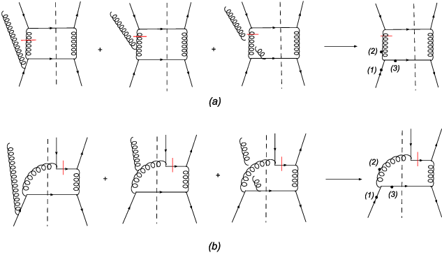
To obtain the SFP cross section, one needs to calculate the diagrams with an extra coherent-gluon line as shown in Fig. 1 with $k_{i}=x_{i}p$ ($i=1,\ 2$). Those diagrams are classified into two types, typical examples of which are shown in Fig. 2. Fig. 2(a) shows the diagrams where the extra gluon line is attached to the cut diagram representing a twist-2 hard cross section. The line with a bar denotes the propagator generating a SFP. For each twist-2 diagram, there are three ways of attaching the coherent gluon, and thus we denote the sum of those three diagrams by a single diagram as shown in the right side of Fig. 2(a) where three dots on the internal lines represent the places to which the gluon line is attached. The mirror diagrams of Fig. 2(a) also give rise to the SFP contribution, and should be included in the calculation. Each of those mirror diagrams give the same result for the SFP cross section as the original diagrams.

The diagrams shown in Fig. 2(b) have the quark and anti-quark lines from the polarized proton in the same side of the final-state cut, and the coherent gluon line is attached to the other side of the cut. Most of this type of diagrams are obtained by shifting the position of the final-state cut in the diagrams shown in Fig. 2(a). For these diagrams, there are again three ways of attaching the coherent gluon line, and we denote the sum of those three by a single diagram with three dots shown in the right side of Fig. 2(b). For the SFP cross section, some contributions in the same channel from the two types of diagrams shown in Figs. 2(a) and (b) cancel each other, as was the case for SIDIS [38], which makes the calculation simpler [41].

Figs. 3$\sim$8 show the diagrams for the SFP contributions ($S_{\alpha}^{\rm SFP}(x_{1}p,x_{2}p,x^{\prime}p^{\prime},P_{h}/z)$ in (9)). Three or four dots numbered as $(1)\sim(4)$ in each diagram represent places where the coherent gluon is attached as explained in Fig. 2. Some diagrams in the figures have 4 dots, since the coupling of the coherent gluon through the 4-gluon vertex has to be taken into account for those diagrams. In Figs. 3$\sim$8, we have only shown the diagrams which represent SFP partonic hard cross sections for the “quark” distribution $G_{F}^{a}(0,x)$ and $\widetilde{G}_{F}^{a}(0,x)$ with $x>0$. By reversing the direction of the arrows of all the fermion lines in each diagram, one obtain the hard cross sections for the “anti-quark” twist-3 distributions defined in (4).

Figs. 3$\sim$6 represent diagrams in the channels with quark or anti-quark distribution for the unpolarized nucleon. Fig. 3 represents diagrams of the type Fig. 2(a) and Fig. 4 represents those of the type Fig. 2(b) in the quark (or anti-quark) fragmentation channel. Fig. 5 represents diagrams of the type Fig. 2(b) and Fig. 6 represents those of the type Fig. 2(a) in the gluon fragmentation channel. Fig. 7 represents diagrams with the gluon distribution for the unpolarized nucleon and quark (or anti-quark) fragmentation function for the pion. Fig. 8 represents those with the gluon distribution for the unpolarized nucleon and the gluon fragmentation function for the pion. In Figs. 3$\sim$8, we have omitted the diagrams which cancel each other as was observed for SIDIS [38, 41].

By calculating all these diagrams, we have eventually obtained the following cross section for the SFP contribution [40, 41]:

where the Mandelstam variables for the process are defined as $S=(p+p^{\prime})^{2}=2p\cdot p^{\prime}$, $T=(p-P_{h})^{2}=-2p\cdot P_{h}$ and $U=(p^{\prime}-P_{h})^{2}=-2p^{\prime}\cdot P_{h}$, $q^{b}(x^{\prime})$ denotes unpolarized quark distribution for the quark flavor $b$, $G(x^{\prime})$ denotes unpolarized gluon distribution, and $D^{i}(z)$ ($i=c$ for the quark-flavor and $i=g$ for gluon) is the pion fragmentation function. In the summations $\sum_{a,b,c}$, $\sum_{a,b}$, $\sum_{a,c}$ and $\sum_{a}$, the sum of $a$ should be taken over all quark and anti-quark flavors ($a=u,d,s,\bar{u},\bar{d},\bar{s},\cdots$) and the sum of $b$ and $c$ is restricted onto quark flavors when $a$ is a quark and onto anti-quark flavors when $a$ is an anti-quark. (For an anti-quark $b$, $\bar{b}$ denotes quark flavor.) The integration region in the convolution formula is specified by $x^{\prime}_{min}=\frac{-T/z}{S+U/z}$ and $z_{min}=-\frac{(T+U)}{S}$. $\hat{\sigma}_{ab\to c}$ etc represents partonic hard cross sections which are the functions of Mandelstam variables in the parton level $\hat{s}=(xp+x^{\prime}p^{\prime})^{2}=xx^{\prime}S$, $\hat{t}=(xp-P_{h}/z)^{2}=\frac{x}{z}T$ and $\hat{u}=(x^{\prime}p^{\prime}-P_{h}/z)^{2}=\frac{x^{\prime}}{z}U$ and are given as follows:

where $N=3$ is the number of colors. A remarkable feature of (10) is that the partonic hard cross sections for $G_{F}(0,x)$ and $\widetilde{G}_{F}(0,x)$ are the same, even though each diagram in Figs. 3$\sim$8 gives different contributions for the two functions. Accordingly, they appear in the combination of $G_{F}(0,x)+\widetilde{G}_{F}(0,x)$ in (10). Although we expect there is a reason for this simple result, we do not understand the origin at this point. Another important feature is that some terms in the hard cross section (the first terms in $\hat{\sigma}_{ab\to c}$, $\hat{\sigma}_{a\bar{b}\to c}$, $\hat{\sigma}_{ag\to c}$ etc.) have the same $1/\hat{t}^{3}$ behavior as the SGP hard cross section which gives dominant contribution to $A_{N}$ in the forward region ($x_{F}\to 1$). In addition their color factors are typically $N^{2}=9$ times larger than those in the SGP cross section, making the magnitude of the SFP hard cross section huge. This suggests that the SFP contribution gives rise to a significant contribution to the asymmetry at large $x_{F}$ even though the SFP function does not appear with the derivative.

To see the impact of the SFP contribution, we have performed a numerical calculation of $A_{N}$ for $p^{\uparrow}p\to\pi X$, assuming that the SFP function is of the same order of magnitude as the SGP function. Kouvaris et al. [31] have parametrized the SGP function $G_{F}^{a}(x,x)$ so that the SGP contribution reproduces the $A_{N}$ data obtained from RHIC and FNAL data. Their analysis shows that both data are reasonably well reproduced. In particular, they found that the derivative term in (5) brings dominant contribution compared to the nonderivative contribution. Here we adopt Fit(I) of [31] and assume $G_{F}^{a}(0,x)+\widetilde{G}_{F}^{a}(0,x)=G_{F}^{a}(x,x)$ ($a=u,d$). Fig. 9 shows $A_{N}$ for the pion at $\sqrt{S}=200$ GeV and $P_{hT}=1.5$ GeV with and without SFP contribution. As is seen from the figure that the SFP contribution brings large effect in the positive $x_{F}$ region, while its effect is negligible in the negative $x_{F}$ region. This is due to the large color factors for the $1/\hat{t}^{3}$ terms in $\hat{\sigma}_{ab\to c}$, $\hat{\sigma}_{a\bar{b}\to c}$, $\hat{\sigma}_{ag\to c}$ as noted above. From this figure it is clear that the SFP contribution can affect $A_{N}$ significantly even though it does not receive enhancement by the derivative unlike SGP contribution, unless the SFP function itself is small. The detail of the present calculation together with a phenomenological analysis of the data will be presented elsewhere [41].

To summarize, we have calculated the SFP contribution to the cross section for $p^{\uparrow}p\to hX$ associated with the twist-3 quark-gluon correlation functions in the polarized nucleon. We have also shown that its effect is significant and should be included in the analysis of $A_{N}$. For a more complete analysis, one needs to include the contribution from the triple-gluon twist-3 distribution function as well. Recent study [36] shows that $A_{N}$ for the open charm production has a potential to determine the function. We hope that the global analysis of all those data including all the QCD effects will clarify the origin of observed SSA.

The work of Y. K. is supported in part by the Uchida Energy Science Promotion Foundation.

References

- [1] D. L. Adams et al., Phys. Lett. B261 (1991) 201; ibid 264 (1991) 462.
- [2]
M. Anselmino, A. Efremov and E. Leader, Phys. Rept. 261
(1995) 1 [Erratum-ibid. 281 (1997) 399];
Z. t. Liang and C. Boros, Int. J. Mod. Phys. A15 (2000) 927;
V. Barone, A. Drago and P. G. Ratcliffe, Phys. Rep. 359 (2002) 1;
U. D’Alesio, F. Murgia, Prog. Part. Nucl. Phys. 61 (2008) 394. - [3] G.L. Kane, J. Pumplin and W. Repko, Phys. Rev. Lett. 41 (1978) 1689.
- [4]
G. Bunce et al., Phys. Rev. Lett. 36 (1976) 1113;
A. M. Smith et al., Phys. Lett. B185 (1987) 209;
B. Lundberg et al., Phys. Rev. D40 (1989) 3557;
E. J. Ramberg et al., Phys. Lett. B338 (1994) 403. - [5]
J. Adams et al. [STAR Collaboration], Phys. Rev. Lett. 92 (2004) 171801;
B.I. Abelev et al. [STAR collaboration], Phys. Rev. Lett. 101 (2008) 222001. - [6] S. S. Adler et al. [PHENIX Collaboration], Phys. Rev. Lett. 95 (2005) 202001.
- [7] I. Arsense et al. [BRAHMS collaboration], Phys. Rev. Lett. 101 (2008) 042001.
- [8]
A. Airapetian et al. [HERMES Collaboration],
Phys. Rev. D 64 (2001) 097101;
Phys. Rev. Lett. 94 (2005) 012002;
M. Diefenthaler [HERMES Collaboration], AIP Conf. Proc. 792 (2005) 933 [hep-ex/0507013]. - [9]
V. Y. Alexakhin et al. [COMPASS Collaboration],
Phys. Rev. Lett. 94 (2005) 202002;
E.S. Ageev et al. [COMPASS Collaboration], Nucl. Phys. B765 (2007) 31. - [10] D. W. Sivers, Phys. Rev. D41 (1990) 83; Phys. Rev. D43 (1991) 261.
- [11] J. C. Collins, Nucl. Phys. B396 (1993) 161.
- [12]
M. Anselmino, M. Boglione and F. Murgia, Phys. Lett. B 362 (1995) 164;
M. Anselmino and F. Murgia, Phys. Lett. B 442 (1998) 470;
M. Anselmino, M. Boglione, U. D’Alesio, A. Kotzinian, F. Murgia and A. Prokudin, Phys. Rev. D 72 (2005) 094007, [Erratum-ibid. D 72 (2005) 099903];
M. Anselmino, M. Boglione, U. D’Alesio, S. Melis, F. Murgia and A. Prokudin, arXiv:0901.3078 [hep-ph], and references quoted therein. - [13] A. V. Efremov and O. V. Teryaev, Sov. J. Nucl. Phys. 36 (1982) 140 [Yad. Phiz. 36 (1982) 242]; Phys. Lett. B150 (1985) 383.
- [14] J. Qiu and G. Sterman, Nucl. Phys. B378 (1992) 52.
- [15] H. Eguchi, Y. Koike and K. Tanaka, Nucl. Phys. B763 (2007) 198.
- [16] J. C. Collins, Phys. Lett. B536 (2002) 43.
- [17] A. V. Belitsky, X. D. Ji, and F. Yuan, Nucl. Phys. B656 (2003) 165.
- [18] D. Boer, P. Mulders and F. Pijlman, Nucl. Phys. B667 (2003) 201.
- [19] J. C. Collins and A. Metz, Phys. Rev. Lett. 93 (2004) 252001.
- [20]
C. J. Bomhof, P. J. Mulders and F. Pijlman, Phys. Lett. B596 (2004) 277;
Eur. Phys. J. C47 (2006) 147.
A. Bacchetta, C. J. Bomhof, P. J. Mulders and F. Pijlman, Phys. Rev. D72 (2005) 034030.
C.J. Bomhof and P.J. Mulders, JHEP 0702:029 (2007); Nucl. Phys. B 795 (2008) 409. - [21] J.C. Collins and D.E. Soper, Nucl. Phys. B193 (1981) 381; B213 (1983) 545(E).
- [22] J.C. Collins, D.E. Soper and G. Sterman, Nucl. Phys. B250 (1985) 199.
- [23] X. D. Ji, J. P. Ma and F. Yuan, Phys. Rev. D71 (2005) 034005; Phys. Lett. B597 (2004) 299.
- [24] X. D. Ji, J. W. Qiu, W. Vogelsang and F. Yuan, Phys. Rev. Lett. 97 (2006) 082002; Phys. Rev. D73 (2006) 094017.
- [25]
Y. Koike, in Proceedings of the RBRC workshop
“Single Spin Asymmetries” (BNL, Upton, New York, June 1-3, 2005)
Vol. 75 (BNL-74717-2005) 33.
H. Eguchi, Y. Koike and K. Tanaka, Nucl. Phys. B752 (2006) 1. - [26] X. D. Ji, J. W. Qiu, W. Vogelsang and F. Yuan, Phys. Lett. B638 (2006) 178.
- [27] Y. Koike and K. Tanaka, Phys. Lett. B 646 (2007) 232 [Erratum-ibid. B 668 (2008) 458]
- [28] J. Qiu and G. Sterman, Phys. Rev. D59 (1999) 014004.
- [29] Y. Kanazawa and Y. Koike, Phys. Lett. B478 (2000) 121; Phys. Lett. B490 (2000) 99.
- [30] Y. Koike, AIP Conf. Proc. 675 (2003) 449 [hep-ph/0210396]; Nucl. Phys. A721 (2003) 364.
- [31] C. Kouvaris, J. W. Qiu, W. Vogelsang and F. Yuan, Phys. Rev. D 74 (2006) 114013.
- [32] Y. Koike and K. Tanaka, Phys. Rev. D 76 (2007) 011502
- [33] Y. Kanazawa and Y. Koike, Phys. Rev. D64 (2001) 034019.
- [34] Y. Koike, AIP Conf. Proc. 675 (2003) 574 [hep-ph/0210434].
- [35] J. Zhou, F. Yuan and Z. T. Liang, arXiv:0808.3629 [hep-ph].
- [36]
Z. B. Kang and J. W. Qiu,
Phys. Rev. D 78 (2008) 034005.
Z. B. Kang, J. W. Qiu, W. Vogelsang and F. Yuan, arXiv:0810.3333 [hep-ph]. - [37] F. Yuan and J. Zhou, Phys. Lett. B 668 (2008) 216.
- [38] Y. Koike, W. Vogelsang and F. Yuan, Phys. Lett. B 659 (2008) 878.
- [39] S. Meissner and A. Metz, arXiv:0812.3783 [hep-ph].
- [40] Y. Koike and T. Tomita, Proceedings of the 18-th international symposium on spin physics (SPIN2008), Univ. of Virginia, Oct. 6-11, 2009. arXiv:0901.2756 [hep-ph].
- [41] Y. Koike and T. Tomita, in preparation.