跳到论文正文
W Papers独立论文阅读器 arXiv:0903.1917 论文正文 计算阅读时间 · 0%
引用这篇论文根据当前论文元数据生成,正式投稿前建议核对。


License: arXiv.org perpetual non-exclusive license
arXiv:0903.1917v3 [hep-ph] 07 Jul 2009

Radiative and Semileptonic BB Decays Involving the Tensor Meson K2∗​(1430)K_{2}^{*}(1430) in the Standard Model and Beyond

Hisaki Hatanaka Affiliation: Department of Physics, Chung-Yuan Christian University, Chung-Li, Taiwan 320, R.O.C.    Kwei-Chou Yang Affiliation: Department of Physics, Chung-Yuan Christian University, Chung-Li, Taiwan 320, R.O.C.
August 24, 2026
Abstract

We study semileptonic and radiative BB decays involving the strange tensor meson K2∗​(1430)K_{2}^{*}(1430) in the final state. Using the large energy effective theory (LEET) techniques, we formulate the B→K2∗B\to K_{2}^{*} transition form factors in large recoil region. All the form factors can be parametrized in terms of two independent LEET functions ζ⟂\zeta_{\perp} and ζ∥\zeta_{\parallel}. The magnitude of ζ⟂\zeta_{\perp} is estimated from the data for ℬ⁡(B→K2∗​(1430)​γ){\cal B}(B\to K_{2}^{*}(1430)\gamma). Assuming a dipole q2q^{2}-dependence for the LEET functions and ζ∥/ζ⟂=1.0±0.2\zeta_{\parallel}/\zeta_{\perp}=1.0\pm 0.2, for which the former consists with the QCD counting rules and the latter is favored by the B→ϕ​K2∗B\to\phi K_{2}^{*} data, we investigate the decays B→K2∗​ℓ+​ℓ−B\to K_{2}^{*}\ell^{+}\ell^{-} and B→K2∗​ν​ν¯B\to K_{2}^{*}\nu\bar{\nu}, where the contributions due to ζ∥\zeta_{\parallel} are suppressed by mK2∗/mBm_{K_{2}^{*}}/m_{B}. For the B→K2∗​ℓ+​ℓ−B\to K_{2}^{*}\ell^{+}\ell^{-} decay, in the large recoil region where the hadronic uncertainties are considerably reduced, the longitudinal distribution d​FL/d​sdF_{L}/ds is reduced by 20−3020-30% due to the flipped sign of c7effc_{7}^{\rm eff} compared with the standard model result. Moreover, the forward-backward asymmetry zero is about 3.4 GeV2 in the standard model, but changing the sign of c7effc_{7}^{\rm eff} yields a positive asymmetry for all values of the invariant mass of the lepton pair. We calculate the branching fraction for B→K2∗​ν​ν¯B\to K_{2}^{*}\nu\bar{\nu} in the standard model. Our result exhibits the impressed resemblance between B→K2∗​(1430)​ℓ+​ℓ−B\to K_{2}^{*}(1430)\ell^{+}\ell^{-}, ν​ν¯\nu\bar{\nu} and B→K∗​(892)​ℓ+​ℓ−B\to K^{*}(892)\ell^{+}\ell^{-}, ν​ν¯\nu\bar{\nu}.

pacs
13.20.He, 14.40.Ev, 12.39.Hg

I Introduction

Table 1: Branching fractions of radiative and semileptonic BB decays involving K∗K^{*} or K2∗K_{2}^{*} .
Mode ℬ{\cal B} [10−610^{-6}] Mode ℬ{\cal B} [10−610^{-6}]
B+→K∗⁣+​(892)​γB^{+}\to K^{*+}(892)\gamma 45.7±1.945.7\pm 1.9 [5, 6, 7] B0→K∗0​(892)​γB^{0}\to K^{*0}(892)\gamma 44.0±1.544.0\pm 1.5 [5, 6, 7]
B+→K2∗⁣+​(1430)​γB^{+}\to K_{2}^{*+}(1430)\gamma 14.5±4.314.5\pm 4.3 [8] B0→K2∗0​(1430)​γB^{0}\to K_{2}^{*0}(1430)\gamma 12.4±2.412.4\pm 2.4 [8, 9]
B+→K∗⁣+​(892)​e+​e−B^{+}\to K^{*+}(892)e^{+}e^{-} 1.42−0.39+0.431.42^{+0.43}_{-0.39} [10, 11] B0→K∗0​(892)​e+​e−B^{0}\to K^{*0}(892)e^{+}e^{-} 1.13−0.18+0.211.13^{+0.21}_{-0.18} [10, 11]
B+→K∗⁣+​(892)​μ+​μ−B^{+}\to K^{*+}(892)\mu^{+}\mu^{-} 1.12−0.27+0.321.12^{+0.32}_{-0.27} [10, 11, 12] B0→K∗0​(892)​μ+​μ−B^{0}\to K^{*0}(892)\mu^{+}\mu^{-} 1.00−0.13+0.151.00^{+0.15}_{-0.13} [10, 11, 12]
B+→K∗⁣+​(892)​ν​ν¯B^{+}\to K^{*+}(892)\nu\bar{\nu} <80<80 [13, 14] B0→K∗0​(892)​ν​ν¯B^{0}\to K^{*0}(892)\nu\bar{\nu} <120<120 [13, 14]

The flavor-changing neutral current (FCNC) processes involving b→s⁡(d)b\to s(d) transitions occur only at loop-level in the standard model (SM) and thus provide an important testing ground to look for new physics phenomena. Radiative BB decays can offer bounds on the CKM matrix elements |Vt​s||V_{ts}| and |Vt​d||V_{td}| as well as powerful constraints on new physics. The absolute value of c7effc_{7}^{{\rm eff}}, which is the Wilson coefficient of electromagnetic dipole operator, extracted from the current B→Xs​γB\to X_{s}\gamma data is consistent with the SM prediction within errors.

The b→s​ℓ+​ℓ−b\to s\ell^{+}\ell^{-} processes arise from photonic penguin, ZZ-penguin and WW-box diagrams. The inclusive B→Xs​ℓ+​ℓ−B\to X_{s}\ell^{+}\ell^{-} and exclusive B→K(∗)​ℓ+​ℓ−B\to K^{(*)}\ell^{+}\ell^{-} decays have been measured [1, 2]. We summarize the current data for branching fractions of exclusive radiative and semileptonic BB decays relevant to the FCNC b→sb\to s transition in Table 1 [3, 4, 5, 6, 7, 8, 9, 10, 11, 12, 13, 14, 15]. The FCNC processes may receive sizable new-physics contributions [17, 18, 16, 19, 20, 21]. Recently, BABAR and Belle have measured interesting observables, K∗K^{*} longitudinal fraction, forward-backward asymmetry and isospin asymmetry, in the B→K∗​ℓ+​ℓ−B\to K^{*}\ell^{+}\ell^{-} decays [3, 15, 1, 2, 10, 11]. Although the data are consistent with the SM predictions, all measurements favor the flipped-sign c7effc_{7}^{\rm eff} models [22]. The minimal flavor violation supersymmetry models with large tan⁡β\tan\beta can be fine-tuned to have the flipped sign of c7effc_{7}^{\rm eff} [24, 23], for which the charged Higgs is dominant. However, the contributions of the charged Higgs exchange to c9c_{9} and c10c_{10} are suppressed by 1/tan2⁡β1/\tan^{2}\beta for large tan⁡β\tan\beta.

The measurements of inclusive and various exclusive decays relevant to FCNC transitions can shed light on new physics. We have studied B→K1​(1270)​γB\to K_{1}(1270)\gamma and B→K1​(1270)​ℓ+​ℓ−B\to K_{1}(1270)\ell^{+}\ell^{-} [25, 26], where the K1​(1270)K_{1}(1270) is the PP-wave meson. B→K1​(1270)​γB\to K_{1}(1270)\gamma has been measured by Belle[27]. In this paper, we focus on the exclusive processes B→K2∗​(1430)​γB\to K_{2}^{*}(1430)\gamma, B→K2∗​(1430)​ℓ+​ℓ−B\to K_{2}^{*}(1430)\ell^{+}\ell^{-} and B→K2∗​(1430)​ν​ν¯B\to K_{2}^{*}(1430)\nu\bar{\nu}, where K2∗​(1430)K_{2}^{*}(1430) is the strange tensor meson with positive parity.

The B→K2∗​(1430)​γB\to K_{2}^{*}(1430)\gamma decays have been observed by Belle and BABAR collaborations [8, 9]. See also Table 1. Corresponding semileptonic decays can be expected to see soon. Because both K2∗K_{2}^{*} and K∗K^{*} mainly decay to the two-body K​πK\pi mode, therefore the angular-distribution analysis for the B→K∗​ℓ+​ℓ−B\to K^{*}\ell^{+}\ell^{-} decays are applicable to the study for B→K2∗​ℓ+​ℓ−B\to K_{2}^{*}\ell^{+}\ell^{-} decays.

In experiments, the exclusive mode is much more easier to accessible than the inclusive process. However, the former contains form factors parametrizing hadronic matrix elements, and thus suffers from large theoretical uncertainties. B→K2∗B\to K_{2}^{*} transition form factors, which are relevant to the study of the radiative and semileptonic BB decays into a K2∗K_{2}^{*}, are less understood compared with B→K∗B\to K^{*} ones. So far only some quark model results about them [28, 29, 30]. In this paper we formulate the B→K2∗B\to K_{2}^{*} form factors in the large recoil region using the large energy effective theory (LEET) techniques [31]. We will show that all the form factors can be parameterized in terms of two independent form factors ζ⟂\zeta_{\perp} and ζ∥\zeta_{\parallel} in the LEET limit. The former form factor can be estimated by using the data for B→K2∗​(1430)​γB\to K_{2}^{*}(1430)\gamma, while the latter only gives corrections of order mK2∗/mBm_{K_{2}^{*}}/m_{B} in the amplitude.

We study the longitudinal distribution d​FL/d​sdF_{L}/ds and forward-backward asymmetry for the B→K2∗​ℓ+​ℓ−B\to K_{2}^{*}\ell^{+}\ell^{-} decay. Particularly, we find that in the large recoil region, where the uncertainties of these observables arising from the form factors are considerably reduced not only due to taking the ratio of form factors but also due to the evaluation in the large EK2∗E_{K_{2}^{*}} limit. For the new-physics effect, we will focus on the possible correction due to the c7effc_{7}^{\rm eff} with the sign flipped.

We calculate the branching fraction for B→K2∗​ν​ν¯B\to K_{2}^{*}\nu\bar{\nu} in the SM. This mode enhanced by the summation over three light neutrinos is theoretically cleaner due to the absence of long-distance corrections related to the relevant four-fermion operators. This decay is relevant for the nonstandard Z0Z^{0} coupling [32], light dark matter [33] and unparticles [34, 35].

The paper is organized as follows. In Sec. II we formulate the B→TB\to T form factors using the LEET techniques. In Sec. III, we numerically study the radiative and semileptonic BB meson decays into the K2∗​(1430)K_{2}^{*}(1430). We conclude with a summary in Sec. IV.

II B→TB\to T form factors in the LEET

For simplicity we work in the rest frame of the BB meson (with mass mBm_{B}) and assume that the light tensor meson TT (with mass mTm_{T}) moves along the zz-axis. The momenta of the BB and TT are given by

pBμ=(mB,0,0,0)≡mB​vμ,pTμ=(E,0,0,p3)≡E​nμ,\displaystyle p_{B}^{\mu}=(m_{B},0,0,0)\equiv m_{B}\,v^{\mu},\quad p_{T}^{\mu}=(E,0,0,p_{3})\equiv E\,n^{\mu}, (1)

respectively. Here the tensor meson’s energy EE is given by

E=mB2​(1−q2mB2+mT2mB2),\displaystyle E=\frac{m_{B}}{2}\left(1-\frac{q^{2}}{m_{B}^{2}}+\frac{m_{T}^{2}}{m_{B}^{2}}\right), (2)

where q≡pB−pTq\equiv p_{B}-p_{T}. In the LEET limit,

E,mB≫mT,ΛQCD,\displaystyle E,m_{B}\gg m_{T},\Lambda_{{\rm QCD}}, (3)

we simply have

vμ=(1,0,0,0),nμ≃(1,0,0,1).\displaystyle v^{\mu}=(1,0,0,0),\quad n^{\mu}\simeq(1,0,0,1). (4)

The polarization tensors ε​(λ)μ​ν\varepsilon(\lambda)^{\mu\nu} of the massive spin-2 tensor meson with helicity λ\lambda can be constructed in terms of the polarization vectors of a massive vector state [36]

ε​(0)∗μ=(p3,0,0,E)/mT,ε​(±)∗μ=(0,∓1,+i,0)/2,\displaystyle\varepsilon(0)^{*\mu}=(p_{3},0,0,E)/m_{T},\quad\varepsilon(\pm)^{*\mu}=(0,\mp 1,+i,0)/\sqrt{2}, (5)

and are given by

εμ​ν​(±2)\displaystyle\varepsilon^{\mu\nu}(\pm 2) ≡\displaystyle\equiv ε​(±)μ​ε​(±)ν,\displaystyle\varepsilon(\pm)^{\mu}\varepsilon(\pm)^{\nu}, (6)
εμ​ν​(±1)\displaystyle\varepsilon^{\mu\nu}(\pm 1) ≡\displaystyle\equiv 12​(ε​(±)μ​ε​(0)ν+ε​(0)μ​ε​(±)ν),\displaystyle\sqrt{\frac{1}{2}}(\varepsilon(\pm)^{\mu}\varepsilon(0)^{\nu}+\varepsilon(0)^{\mu}\varepsilon(\pm)^{\nu}), (7)
εμ​ν​(0)\displaystyle\varepsilon^{\mu\nu}(0) ≡\displaystyle\equiv 16​(ε​(+)μ​ε​(−)ν+ε​(−)μ​ε​(+)ν)+23​ε​(0)μ​ε​(0)ν.\displaystyle\sqrt{\frac{1}{6}}(\varepsilon(+)^{\mu}\varepsilon(-)^{\nu}+\varepsilon(-)^{\mu}\varepsilon(+)^{\nu})+\sqrt{\frac{2}{3}}\varepsilon(0)^{\mu}\varepsilon(0)^{\nu}. (8)

Due to the purpose of the present study, we calculate the B¯→T\overline{B}\to T transition form factors:

⟨T|Vμ|B¯⟩,⟨T|Aμ|B¯⟩,⟨T|Tμ​ν|B¯⟩,⟨T​|T5μ​ν|​B¯⟩,\displaystyle{\langle{T}}|V^{\mu}|{{\overline{B}}\rangle},\quad{\langle{T}}|A^{\mu}|{{\overline{B}}\rangle},\quad{\langle{T}}|T^{\mu\nu}|{{\overline{B}}\rangle},\quad{\langle{T}}|T_{5}^{\mu\nu}|{{\overline{B}}\rangle}, (9)

where Vμ≡ψ¯​γμ​bV^{\mu}\equiv\bar{\psi}\gamma^{\mu}b, Aμ≡ψ¯​γμ​γ5​bA^{\mu}\equiv\bar{\psi}\gamma^{\mu}\gamma_{5}b, Tμ​ν=ψ¯​σμ​ν​bT^{\mu\nu}=\bar{\psi}\sigma^{\mu\nu}b and T5μ​ν=ψ¯​σμ​ν​γ5​bT_{5}^{\mu\nu}=\bar{\psi}\sigma^{\mu\nu}\gamma_{5}b. There is a trick to write down the form factors in the LEET limit. We first note that we have three independent classes of Lorentz structures (i) ϵα​β​μ​ν\epsilon^{\alpha\beta\mu\nu}, (ii) vμv^{\mu}, nμn^{\mu} and (iii)

2​mTE​{ε​(λ)∗μ​ν​vν−[ε​(λ)α​β∗​vα​vβ]​nμ}\displaystyle\sqrt{2}\frac{m_{T}}{E}\{\varepsilon(\lambda)^{*\mu\nu}v_{\nu}-[\varepsilon(\lambda)^{*}_{\alpha\beta}v^{\alpha}v^{\beta}]n^{\mu}\} =\displaystyle= {0for ​λ=±2,ε​(±)μfor ​λ=±1,0for ​λ=0,\displaystyle\begin{cases}0&\mbox{for }\lambda=\pm 2,\\ \varepsilon(\pm)^{\mu}&\mbox{for }\lambda=\pm 1,\\ 0&\mbox{for }\lambda=0,\end{cases} (10)
2​mTE​ϵμ​ν​ρ​σ​[ε​(λ)ν​α∗​vα]​nρ​vσ\displaystyle\sqrt{2}\frac{m_{T}}{E}\epsilon^{\mu\nu\rho\sigma}[\varepsilon(\lambda)^{*}_{\nu\alpha}v^{\alpha}]n_{\rho}v_{\sigma} =\displaystyle= {0for ​λ=±2,ϵμ​ν​ρ​σ​ε​(±)ν​nρ​vσfor ​λ=±1,0for ​λ=0,\displaystyle\begin{cases}0&\mbox{for }\lambda=\pm 2,\\ \epsilon^{\mu\nu\rho\sigma}\varepsilon(\pm)_{\nu}n_{\rho}v_{\sigma}&\mbox{for }\lambda=\pm 1,\\ 0&\mbox{for }\lambda=0,\end{cases} (11)
32​(mTE)2​[ε​(λ)α​β∗​vα​vβ]​nμ\displaystyle\sqrt{\frac{3}{2}}\left(\frac{m_{T}}{E}\right)^{2}[\varepsilon(\lambda)^{*}_{\alpha\beta}v^{\alpha}v^{\beta}]n^{\mu} =\displaystyle= {0for ​λ=±2,0for ​λ=±1,nμfor ​λ=0,\displaystyle\begin{cases}0&\mbox{for }\lambda=\pm 2,\\ 0&\mbox{for }\lambda=\pm 1,\\ n^{\mu}&\mbox{for }\lambda=0,\end{cases} (12)
32​(mTE)2​[ε​(λ)α​β∗​vα​vβ]​vμ\displaystyle\sqrt{\frac{3}{2}}\left(\frac{m_{T}}{E}\right)^{2}[\varepsilon(\lambda)^{*}_{\alpha\beta}v^{\alpha}v^{\beta}]v^{\mu} =\displaystyle= {0for ​λ=±2,0for ​λ=±1,vμfor ​λ=0,\displaystyle\begin{cases}0&\mbox{for }\lambda=\pm 2,\\ 0&\mbox{for }\lambda=\pm 1,\\ v^{\mu}&\mbox{for }\lambda=0,\end{cases} (13)

to project the relevant polarization states of the tensor meson. Eqs. (10), (12) and (13) are the vectors, but Eq. (11) the axial-vector. Matching the parities of the matrix elements and using the three classes of the Lorentz structures, we can then easily parametrize the form factors in the following results:

⟨T|Vμ|B¯⟩\displaystyle{\langle{T}}|V^{\mu}|{{\overline{B}}\rangle} =\displaystyle= −i​2​E​(mTE)​ζ⟂(v)​ε∗μ​ν​ρ​σ​vν​nρ​εσ​β∗​vβ,\displaystyle-i2E\left(\frac{m_{T}}{E}\right)\zeta^{(v)}_{\perp}\varepsilon^{*\mu\nu\rho\sigma}v_{\nu}n_{\rho}\varepsilon^{*}_{\sigma\beta}v^{\beta}, (14)
⟨T|Aμ|B¯⟩\displaystyle{\langle{T}}|A^{\mu}|{{\overline{B}}\rangle} =\displaystyle= 2​E​(mTE)​ζ⟂(a)​[ε∗μ​α​vα−(εα​β∗​vα​vβ)​nμ]\displaystyle 2E\left(\frac{m_{T}}{E}\right)\zeta^{(a)}_{\perp}\left[\varepsilon^{*\mu\alpha}v_{\alpha}-(\varepsilon^{*}_{\alpha\beta}v^{\alpha}v^{\beta})n^{\mu}\right] (15)
+2E(mT2E2)(εα​β∗vαvβ)[ζ∥(a)nμ+ζ∥,1(a)vμ],\displaystyle+2E\left(\frac{m_{T}^{2}}{E^{2}}\right)(\varepsilon^{*}_{\alpha\beta}v^{\alpha}v^{\beta})\left[\zeta^{(a)}_{\parallel}n^{\mu}+\zeta^{(a)}_{\parallel,1}v^{\mu}\right],
⟨T|Tμ​ν|B¯⟩\displaystyle{\langle{T}}|T^{\mu\nu}|{{\overline{B}}\rangle} =\displaystyle= 2​E​(mT2E2)​ζ∥(t)​ϵμ​ν​ρ​σ​(εα​β∗​vα​vβ)​vρ​nσ\displaystyle 2E\left(\frac{m_{T}^{2}}{E^{2}}\right)\zeta^{(t)}_{\parallel}\epsilon^{\mu\nu\rho\sigma}(\varepsilon^{*}_{\alpha\beta}v^{\alpha}v^{\beta})v_{\rho}n_{\sigma} (16)
+2​E​(mTE)​ζ⟂(t)​ϵμ​ν​ρ​σ​nρ​[εσ​α∗​vα−(εα​β∗​vα​vβ)​nσ]\displaystyle+2E\left(\frac{m_{T}}{E}\right)\zeta^{(t)}_{\perp}\epsilon^{\mu\nu\rho\sigma}n_{\rho}[\varepsilon^{*}_{\sigma\alpha}v^{\alpha}-(\varepsilon^{*}_{\alpha\beta}v^{\alpha}v^{\beta})n_{\sigma}]
+2​E​(mTE)​ζ⟂,1(t)​ϵμ​ν​ρ​σ​vρ​[εσ​α∗​vα−(εα​β∗​vα​vβ)​nσ],\displaystyle+2E\left(\frac{m_{T}}{E}\right)\zeta^{(t)}_{\perp,1}\epsilon^{\mu\nu\rho\sigma}v_{\rho}[\varepsilon^{*}_{\sigma\alpha}v^{\alpha}-(\varepsilon^{*}_{\alpha\beta}v^{\alpha}v^{\beta})n_{\sigma}],
⟨T|T5μ​ν|B¯⟩\displaystyle{\langle{T}}|T_{5}^{\mu\nu}|{{\overline{B}}\rangle} =\displaystyle= −i​2​E​(mTE)​ζ⟂,1(t5)​{[ε∗μ​α​vα−(εα​β∗​vα​vβ)​nμ]​vν−(μ↔ν)}\displaystyle-i2E\left(\frac{m_{T}}{E}\right)\zeta^{(t_{5})}_{\perp,1}\left\{\left[\varepsilon^{*\mu\alpha}v_{\alpha}-(\varepsilon^{*}_{\alpha\beta}v^{\alpha}v^{\beta})n^{\mu}\right]v^{\nu}-(\mu\leftrightarrow\nu)\right\} (17)
−i​2​E​(mTE)​ζ⟂(t5)​{[ε∗μ​α​vα−(εα​β∗​vα​vβ)​nμ]​nν−(μ↔ν)}\displaystyle-i2E\left(\frac{m_{T}}{E}\right)\zeta^{(t_{5})}_{\perp}\left\{\left[\varepsilon^{*\mu\alpha}v_{\alpha}-(\varepsilon^{*}_{\alpha\beta}v^{\alpha}v^{\beta})n^{\mu}\right]n^{\nu}-(\mu\leftrightarrow\nu)\right\}
−i​2​E​(mT2E2)​ζ∥(t5)​(εα​β∗​vα​vβ)​(nμ​vν−nν​vμ),\displaystyle-i2E\left(\frac{m_{T}^{2}}{E^{2}}\right)\zeta^{(t_{5})}_{\parallel}(\varepsilon^{*}_{\alpha\beta}v^{\alpha}v^{\beta})(n^{\mu}v^{\nu}-n^{\nu}v^{\mu}),

where ϵ0123=−1\epsilon^{0123}=-1 is adopted. ⟨T|Tμ​ν|B¯⟩{\langle{T}}|T^{\mu\nu}|{{\overline{B}}\rangle} is related to ⟨T|T5μ​ν|B¯⟩{\langle{T}}|T_{5}^{\mu\nu}|{{\overline{B}}\rangle} by using the relation: σμ​ν​γ5​ϵμ​ν​ρ​σ=2​i​σρ​σ\sigma^{\mu\nu}\gamma_{5}\epsilon_{\mu\nu\rho\sigma}=2i\sigma_{\rho\sigma}. Note that for the tensor meson only the states with helicities ±1\pm 1 and 00 contribute to the B¯→T\overline{B}\to T transition in the LEET limit. ζ⟂\zeta_{\perp}’s are relevant to TT with helicity =±1=\pm 1, and ζ∥\zeta_{\parallel}’s to TT with helicity =0=0.

In order to reduce the number of the independent B¯→T\overline{B}\to T form factors, we consider the effective current operator q¯n​Γ​bv\bar{q}_{n}\Gamma b_{v} (with Γ=1,γ5,γμ,γμ​γ5,σμ​ν,σμ​ν​γ5\Gamma=1,\gamma_{5},\gamma^{\mu},\gamma^{\mu}\gamma_{5},\sigma^{\mu\nu},\sigma^{\mu\nu}\gamma_{5}) in the LEET limit, instead of the original one q¯​Γ​b\bar{q}\Gamma b [31]. Here bvb_{v} and qnq_{n} satisfy  / ​v​bv=bv\hbox to0.0pt{\hbox to5.20601pt{\hfil/\hfil}\hss}vb_{v}=b_{v},  / ​n​qn=0\hbox to0.0pt{\hbox to6.00235pt{\hfil/\hfil}\hss}nq_{n}=0 and ( / ​n​ / ​v/2)​qn=qn(\hbox to0.0pt{\hbox to6.00235pt{\hfil/\hfil}\hss}n\hbox to0.0pt{\hbox to5.20601pt{\hfil/\hfil}\hss}v/2)q_{n}=q_{n}. Employing the Dirac identities

 / ​v​ / ​n2​γμ\displaystyle\frac{\hbox to0.0pt{\hbox to5.20601pt{\hfil/\hfil}\hss}v\hbox to0.0pt{\hbox to6.00235pt{\hfil/\hfil}\hss}n}{2}\gamma^{\mu} =\displaystyle=  / ​v​ / ​n2​(nμ​ / ​v−i​ϵμ​ν​ρ​σ​vν​nρ​γσ​γ5),\displaystyle\frac{\hbox to0.0pt{\hbox to5.20601pt{\hfil/\hfil}\hss}v\hbox to0.0pt{\hbox to6.00235pt{\hfil/\hfil}\hss}n}{2}\left(n^{\mu}\hbox to0.0pt{\hbox to5.20601pt{\hfil/\hfil}\hss}v-i\epsilon^{\mu\nu\rho\sigma}v_{\nu}n_{\rho}\gamma_{\sigma}\gamma_{5}\right), (18)
 / ​v​ / ​n2​σμ​ν\displaystyle\frac{\hbox to0.0pt{\hbox to5.20601pt{\hfil/\hfil}\hss}v\hbox to0.0pt{\hbox to6.00235pt{\hfil/\hfil}\hss}n}{2}\sigma^{\mu\nu} =\displaystyle=  / ​v​ / ​n2​[i⁡(nμ​vν−nν​vμ)−i⁡(nμ​γν−nν​γμ)​ / ​v−ϵμ​ν​ρ​σ​vν​nρ​γσ​γ5],\displaystyle\frac{\hbox to0.0pt{\hbox to5.20601pt{\hfil/\hfil}\hss}v\hbox to0.0pt{\hbox to6.00235pt{\hfil/\hfil}\hss}n}{2}\left[i(n^{\mu}v^{\nu}-n^{\nu}v^{\mu})-i(n^{\mu}\gamma^{\nu}-n^{\nu}\gamma^{\mu})\hbox to0.0pt{\hbox to5.20601pt{\hfil/\hfil}\hss}v-\epsilon^{\mu\nu\rho\sigma}v_{\nu}n_{\rho}\gamma_{\sigma}\gamma_{5}\right], (19)

where ϵ0123=−1\epsilon^{0123}=-1 is adopted, one can obtain the following relations:

q¯n​bv\displaystyle\bar{q}_{n}b_{v} =\displaystyle= vμ​q¯n​γμ​bv,\displaystyle v_{\mu}\bar{q}_{n}\gamma^{\mu}b_{v}, (20)
q¯n​γμ​bv\displaystyle\bar{q}_{n}\gamma^{\mu}b_{v} =\displaystyle= nμ​q¯n​bv−i​ϵμ​ν​ρ​σ​vν​nρ​q¯n​γσ​γ5​bv,\displaystyle n^{\mu}\bar{q}_{n}b_{v}-i\epsilon^{\mu\nu\rho\sigma}v_{\nu}n_{\rho}\bar{q}_{n}\gamma_{\sigma}\gamma_{5}b_{v}, (21)
q¯n​γμ​γ5​bv\displaystyle\bar{q}_{n}\gamma^{\mu}\gamma_{5}b_{v} =\displaystyle= −nμ​q¯n​γ5​bv−i​ϵμ​ν​ρ​σ​vν​nρ​q¯n​γσ​bv,\displaystyle-n^{\mu}\bar{q}_{n}\gamma_{5}b_{v}-i\epsilon^{\mu\nu\rho\sigma}v_{\nu}n_{\rho}\bar{q}_{n}\gamma_{\sigma}b_{v}, (22)
q¯n​σμ​ν​bv\displaystyle\bar{q}_{n}\sigma^{\mu\nu}b_{v} =\displaystyle= i⁡[nμ​vν​q¯n​bv−nμ​q¯n​γν​bv−(μ↔ν)]−ϵμ​ν​ρ​σ​vρ​nσ​q¯n​γ5​bv,\displaystyle i\left[n^{\mu}v^{\nu}\bar{q}_{n}b_{v}-n^{\mu}\bar{q}_{n}\gamma^{\nu}b_{v}-(\mu\leftrightarrow\nu)\right]-\epsilon^{\mu\nu\rho\sigma}v_{\rho}n_{\sigma}\bar{q}_{n}\gamma_{5}b_{v}, (23)
q¯n​σμ​ν​γ5​bv\displaystyle\bar{q}_{n}\sigma^{\mu\nu}\gamma_{5}b_{v} =\displaystyle= i⁡[nμ​vν​q¯n​γ5​bv+nμ​q¯n​γν​γ5​bv−(μ↔ν)]−ϵμ​ν​ρ​σ​vρ​nσ​q¯n​bv.\displaystyle i\left[n^{\mu}v^{\nu}\bar{q}_{n}\gamma_{5}b_{v}+n^{\mu}\bar{q}_{n}\gamma^{\nu}\gamma_{5}b_{v}-(\mu\leftrightarrow\nu)\right]-\epsilon^{\mu\nu\rho\sigma}v_{\rho}n_{\sigma}\bar{q}_{n}b_{v}. (24)

Substituting the above results into Eqs. (14)-(17), we have

ζ⟂(v)=ζ⟂(a)=ζ⟂(t)=ζ⟂(t5)\displaystyle\zeta^{(v)}_{\perp}=\zeta^{(a)}_{\perp}=\zeta^{(t)}_{\perp}=\zeta^{(t_{5})}_{\perp} ≡\displaystyle\equiv ζ⟂,\displaystyle\zeta_{\perp}, (25)
ζ∥(a)=ζ∥(t)=ζ∥(t5)\displaystyle\zeta^{(a)}_{\parallel}=\zeta^{(t)}_{\parallel}=\zeta^{(t_{5})}_{\parallel} ≡\displaystyle\equiv ζ∥,\displaystyle\zeta_{\parallel}, (26)
ζ(a)∥,1=ζ(t5)⟂,1=ζ(t)⟂,1\displaystyle\zeta^{(a)}_{\parallel,1}=\zeta^{(t_{5})}_{\perp,1}=\zeta^{(t)}_{\perp,1} =\displaystyle= 0,\displaystyle 0, (27)

and thus find that there are only two independent components, ζ⟂​(q2)\zeta_{\perp}(q^{2}) and ζ∥​(q2)\zeta_{\parallel}(q^{2}), for the B→TB\to T transition in the LEET limit. In the full theory, the B¯​(pB)→K¯2∗​(pK2∗,λ)\overline{B}(p_{B})\to\overline{K}_{2}^{*}(p_{K_{2}^{*}},\lambda) form factors are defined as follows,

⟨K¯2∗​(pK2∗,λ)|s¯​γμ​b|B¯​(pB)⟩\displaystyle{\langle{\overline{K}_{2}^{*}(p_{K_{2}^{*}},\lambda)}}|\bar{s}\gamma^{\mu}b|{{\overline{B}(p_{B})}\rangle} =\displaystyle= −i​2mB+mK2∗​V~K2∗​(q2)​ϵμ​ν​ρ​σ​pB​ν​pK2∗​ρ​eσ∗,\displaystyle-i\frac{2}{m_{B}+m_{K_{2}^{*}}}\tilde{V}^{K_{2}^{*}}(q^{2})\epsilon^{\mu\nu\rho\sigma}p_{B\nu}p_{K_{2}^{*}\rho}e^{*}_{\sigma}, (28)
⟨K¯2∗​(pK2∗,λ)|s¯​γμ​γ5​b|B¯​(pB)⟩\displaystyle{\langle{\overline{K}_{2}^{*}(p_{K_{2}^{*}},\lambda)}}|\bar{s}\gamma^{\mu}\gamma_{5}b|{{\overline{B}(p_{B})}\rangle} =\displaystyle= 2​mK2∗​A~0K2∗​(q2)​e∗⋅pBq2​qμ\displaystyle 2m_{K_{2}^{*}}\tilde{A}_{0}^{K_{2}^{*}}(q^{2})\frac{e^{*}\cdot p_{B}}{q^{2}}q^{\mu}
+(mB+mK2∗)​A~1K2∗​(q2)​[e∗μ−e∗⋅pBq2​qμ]\displaystyle+(m_{B}+m_{K_{2}^{*}})\tilde{A}_{1}^{K_{2}^{*}}(q^{2})\left[e^{*\mu}-\frac{e^{*}\cdot p_{B}}{q^{2}}q^{\mu}\right]
−A~2K2∗​(q2)​e∗⋅pBmB+mK2∗​[pBμ+pK2∗μ−mB2−mK2∗2q2​qμ],\displaystyle-\tilde{A}_{2}^{K_{2}^{*}}(q^{2})\frac{e^{*}\cdot p_{B}}{m_{B}+m_{K_{2}^{*}}}\left[p_{B}^{\mu}+p_{K_{2}^{*}}^{\mu}-\frac{m_{B}^{2}-m_{K_{2}^{*}}^{2}}{q^{2}}q^{\mu}\right],
⟨K¯2∗​(pK2∗,λ)|s¯​σμ​ν​qν​b|B¯​(pB)⟩\displaystyle{\langle{\overline{K}_{2}^{*}(p_{K_{2}^{*}},\lambda)}}|\bar{s}\sigma^{\mu\nu}q_{\nu}b|{{\overline{B}(p_{B})}\rangle} =\displaystyle= 2​T~1K2∗​(q2)​ϵμ​ν​ρ​σ​pB​ν​pK2∗​ρ​eσ∗,\displaystyle 2\tilde{T}_{1}^{K_{2}^{*}}(q^{2})\epsilon^{\mu\nu\rho\sigma}p_{B\nu}p_{K_{2}^{*}\rho}e^{*}_{\sigma}, (30)
⟨K¯2∗​(pK2∗,λ)|s¯​σμ​ν​γ5​qν​b|B¯​(pB)⟩\displaystyle{\langle{\overline{K}_{2}^{*}(p_{K_{2}^{*}},\lambda)}}|\bar{s}\sigma^{\mu\nu}\gamma_{5}q_{\nu}b|{{\overline{B}(p_{B})}\rangle} =\displaystyle= −i​T2~K2∗​(q2)​[(mB2−mK2∗2)​e∗μ−(e∗⋅pB)​(pBμ+pK2∗μ)]\displaystyle-i\tilde{T_{2}}^{K_{2}^{*}}(q^{2})\left[(m_{B}^{2}-m_{K_{2}^{*}}^{2})e^{*\mu}-(e^{*}\cdot p_{B})(p_{B}^{\mu}+p_{K_{2}^{*}}^{\mu})\right]
−i​T3~K2∗​(q2)​(e∗⋅pB)​[qμ−q2mB2−mK2∗2​(pBμ+pK2∗μ)],\displaystyle-i\tilde{T_{3}}^{K_{2}^{*}}(q^{2})(e^{*}\cdot p_{B})\left[q^{\mu}-\frac{q^{2}}{m_{B}^{2}-m_{K_{2}^{*}}^{2}}(p_{B}^{\mu}+p_{K_{2}^{*}}^{\mu})\right],

where eμ≡εμ​ν​(pK2∗,λ)​pB,ν/mBe^{\mu}\equiv\varepsilon^{\mu\nu}(p_{K_{2}^{*}},\lambda)p_{B,\nu}/m_{B} corresponding to λ=0,±1\lambda=0,\pm 1. We have eμ=(|p→K2∗|/mK2∗)​ε~μe^{\mu}=(|\vec{p}_{K_{2}^{*}}|/m_{K_{2}^{*}})\tilde{\varepsilon}^{\mu}, where ε~​(0)=2/3​ε​(0)\tilde{\varepsilon}(0)=\sqrt{2/3}\varepsilon(0) and ε~​(±1)=1/2​ε​(±1)\tilde{\varepsilon}(\pm 1)=\sqrt{1/2}\varepsilon(\pm 1). We thus normalize these form factors and obtain relations as follows

A~0K2∗​(q2)​|p→K2∗|mK2∗\displaystyle\tilde{A}_{0}^{K_{2}^{*}}(q^{2})\frac{|\vec{p}_{K_{2}^{*}}|}{m_{K_{2}^{*}}} ≡\displaystyle\equiv A0K2∗​(q2)≃(1−mK2∗2mB​E)​ζ∥​(q2)+mK2∗mB​ζ⟂​(q2),\displaystyle A_{0}^{K_{2}^{*}}(q^{2})\simeq\left(1-\frac{m_{K_{2}^{*}}^{2}}{m_{B}E}\right)\zeta_{\parallel}(q^{2})+\frac{m_{K_{2}^{*}}}{m_{B}}\zeta_{\perp}(q^{2}), (32)
A~1K2∗​(q2)​|p→K2∗|mK2∗\displaystyle\tilde{A}_{1}^{K_{2}^{*}}(q^{2})\frac{|\vec{p}_{K_{2}^{*}}|}{m_{K_{2}^{*}}} ≡\displaystyle\equiv A1K2∗​(q2)≃2​EmB+mK2∗​ζ⟂​(q2),\displaystyle A_{1}^{K_{2}^{*}}(q^{2})\simeq\frac{2E}{m_{B}+m_{K_{2}^{*}}}\zeta_{\perp}(q^{2}), (33)
A~2K2∗​(q2)​|p→K2∗|mK2∗\displaystyle\tilde{A}_{2}^{K_{2}^{*}}(q^{2})\frac{|\vec{p}_{K_{2}^{*}}|}{m_{K_{2}^{*}}} ≡\displaystyle\equiv A2K2∗​(q2)≃(1+mK2∗mB)​[ζ⟂​(q2)−mK2∗E​ζ∥​(q2)],\displaystyle A_{2}^{K_{2}^{*}}(q^{2})\simeq\left(1+\frac{m_{K_{2}^{*}}}{m_{B}}\right)\left[\zeta_{\perp}(q^{2})-\frac{m_{K_{2}^{*}}}{E}\zeta_{\parallel}(q^{2})\right], (34)
V~K2∗​(q2)​|p→K2∗|mK2∗\displaystyle\tilde{V}^{K_{2}^{*}}(q^{2})\frac{|\vec{p}_{K_{2}^{*}}|}{m_{K_{2}^{*}}} ≡\displaystyle\equiv VK2∗​(q2)≃(1+mK2∗mB)​ζ⟂​(q2),\displaystyle V^{K_{2}^{*}}(q^{2})\simeq\left(1+\frac{m_{K_{2}^{*}}}{m_{B}}\right)\zeta_{\perp}(q^{2}), (35)
T~1K2∗​(q2)​|p→K2∗|mK2∗\displaystyle\tilde{T}_{1}^{K_{2}^{*}}(q^{2})\frac{|\vec{p}_{K_{2}^{*}}|}{m_{K_{2}^{*}}} ≡\displaystyle\equiv T1K2∗​(q2)≃ζ⟂​(q2),\displaystyle T_{1}^{K_{2}^{*}}(q^{2})\simeq\zeta_{\perp}(q^{2}), (36)
T~2K2∗​(q2)​|p→K2∗|mK2∗\displaystyle\tilde{T}_{2}^{K_{2}^{*}}(q^{2})\frac{|\vec{p}_{K_{2}^{*}}|}{m_{K_{2}^{*}}} ≡\displaystyle\equiv T2K2∗​(q2)≃(1−q2mB2−mK2∗2)​ζ⟂​(q2),\displaystyle T_{2}^{K_{2}^{*}}(q^{2})\simeq\left(1-\frac{q^{2}}{m_{B}^{2}-m_{K_{2}^{*}}^{2}}\right)\zeta_{\perp}(q^{2}), (37)
T~3K2∗​(q2)​|p→K2∗|mK2∗\displaystyle\tilde{T}_{3}^{K_{2}^{*}}(q^{2})\frac{|\vec{p}_{K_{2}^{*}}|}{m_{K_{2}^{*}}} ≡\displaystyle\equiv T3K2∗​(q2)≃ζ⟂​(q2)−(1−mK2∗2mB2)​mK2∗E​ζ∥​(q2),\displaystyle T_{3}^{K_{2}^{*}}(q^{2})\simeq\zeta_{\perp}(q^{2})-\left(1-\frac{m_{K_{2}^{*}}^{2}}{m_{B}^{2}}\right)\frac{m_{K_{2}^{*}}}{E}\zeta_{\parallel}(q^{2}), (38)

where have used |p→K2∗|/E≃1|\vec{p}_{K_{2}^{*}}|/E\simeq 1. Our results are consistent with Ref. [30]. Defining

ε~​(0)μ=αL​ε​(0)μ,ε~​(±1)μ=βT​ε​(±1)μ,\displaystyle\tilde{\varepsilon}(0)^{\mu}=\alpha_{L}\varepsilon(0)^{\mu},\quad\tilde{\varepsilon}(\pm 1)^{\mu}=\beta_{T}\varepsilon(\pm 1)^{\mu}, (39)

we can easily generalize the studies of B→K∗​γB\to K^{*}\gamma, B→K∗​ℓ+​ℓ−B\to K^{*}\ell^{+}\ell^{-} and B→K∗​ν​ν¯B\to K^{*}\nu\bar{\nu} to B→K2∗​γB\to K_{2}^{*}\gamma, B→K2∗​ℓ+​ℓ−B\to K_{2}^{*}\ell^{+}\ell^{-} and B→K2∗​ν​ν¯B\to K_{2}^{*}\nu\bar{\nu} processes. For the K∗K^{*} cases, we have αL=βT=1\alpha_{L}=\beta_{T}=1, whereas for the K2∗K_{2}^{*} cases, we instead use αL=2/3\alpha_{L}=\sqrt{2/3} and βT=1/2\beta_{T}=1/\sqrt{2}.

III Numerical Study

In the following numerical study, we use the input parameters listed in Table 2. The Wilson coefficients that we adopt are the same as that in Ref. [26]

Table 2: Input parameters
Tensor meson mass mK2∗⁣+​(1430)=1.426​GeVm_{K_{2}^{*+}(1430)}=1.426\,{\rm GeV},  mK2∗0​(1430)=1.432​GeVm_{K_{2}^{*0}(1430)}=1.432\,{\rm GeV},
bb quark mass [37] mb,pole=4.79−0.08+0.19​GeVm_{b,{\rm pole}}=4.79^{+0.19}_{-0.08}\,{\rm GeV},
BB lifetime (picosecond) τB+=1.638\tau_{B^{+}}=1.638,  τB0=1.530\tau_{B^{0}}=1.530,
CKM parameter [38] |Vt​s∗​Vt​b|=0.040±0.001|V_{ts}^{*}V_{tb}|=0.040\pm 0.001,  |Vu​b|=(3.44−0.17+0.22)×10−3|V_{ub}|=(3.44^{+0.22}_{-0.17})\times 10^{-3}.

III.1 B→K2∗​γB\to K_{2}^{*}\gamma and B→K2∗​ℓ+​ℓ−B\to K_{2}^{*}\ell^{+}\ell^{-}

The effective Hamiltonian relevant to the B→K2∗​γB\to K_{2}^{*}\gamma and B→K2∗​ℓ+​ℓ−B\to K_{2}^{*}\ell^{+}\ell^{-} decays is given by

ℋeff\displaystyle{\cal H}_{{\rm eff}} =\displaystyle= −GF2Vt​bVt​s∗∑i=110ci(μ)𝒪i(μ)+H.c.,\displaystyle-\frac{G_{F}}{\sqrt{2}}V_{tb}V_{ts}^{*}\sum_{i=1}^{10}c_{i}(\mu){\cal O}_{i}(\mu)+\mbox{H.c.}, (40)
𝒪7\displaystyle{\cal O}_{7} =\displaystyle= −ge​m​mb8​π2​s¯​σμ​ν​(1+γ5)​b​Fμ​ν,𝒪8=−gs​mb8​π2​s¯i​σμ​ν​(1+γ5)​bj​Gμ​ν​Ti​j,\displaystyle-\frac{g_{em}m_{b}}{8\pi^{2}}\bar{s}\sigma_{\mu\nu}(1+\gamma_{5})bF_{\mu\nu},\quad{\cal O}_{8}=-\frac{g_{s}m_{b}}{8\pi^{2}}\bar{s}_{i}\sigma_{\mu\nu}(1+\gamma_{5})b_{j}G^{\mu\nu}T^{ij},
𝒪9\displaystyle{\cal O}_{9} =\displaystyle= αE​M2​π​s¯​(1−γ5)​b​(ℓ¯​ℓ),𝒪10=αE​M2​π​s¯​(1−γ5)​b​(ℓ¯​γ5​ℓ).\displaystyle\frac{\alpha_{EM}}{2\pi}\bar{s}(1-\gamma_{5})b(\bar{\ell}\ell),\quad{\cal O}_{10}=\frac{\alpha_{EM}}{2\pi}\bar{s}(1-\gamma_{5})b(\bar{\ell}\gamma_{5}\ell). (41)

In analogy to B→K∗​γB\to K^{*}\gamma [24, 40, 39, 41], the B→K2∗​γB\to K_{2}^{*}\gamma decay width reads

Γ⁡(B→K2∗​γ)\displaystyle\Gamma(B\to K_{2}^{*}\gamma) (42)
=\displaystyle= GF2​αE​M​|Vt​s∗​Vt​b|232​π4​mb,pole2​mB3​(1−mK2∗2mB2)3​|c7(0)​eff+A(1)|2​|T1K2∗​(0)|2​βT2,\displaystyle\frac{G_{F}^{2}\alpha_{EM}\left|V_{ts}^{*}V_{tb}\right|^{2}}{32\pi^{4}}m_{b,{\rm pole}}^{2}m_{B}^{3}\left(1-\frac{m_{K_{2}^{*}}^{2}}{m_{B}^{2}}\right)^{3}\left|c_{7}^{(0){{\rm eff}}}+A^{(1)}\right|^{2}\left|T_{1}^{K_{2}^{*}}(0)\right|^{2}\beta_{T}^{2},

with βT=1/2\beta_{T}=\sqrt{1/2}. Here A(1)A^{(1)} is decomposed into the following components [40]

A(1)​(μ)\displaystyle A^{(1)}(\mu) =\displaystyle= Ac7(1)​(μ)+Aver(1)​(μ)=−0.038−0.016​i.\displaystyle A_{c_{7}}^{(1)}(\mu)+A_{\rm ver}^{(1)}(\mu)=-0.038-0.016i. (43)

In the LEET limit, T1K2∗​(q2)T_{1}^{K_{2}^{*}}(q^{2}) can be parametrized in terms of two independent functions ζ⟂​(q2)\zeta_{\perp}(q^{2}) and ζ∥​(q2)\zeta_{\parallel}(q^{2}). Using c7(0)​eff=−0.315c_{7}^{(0){\rm eff}}=-0.315 and the ℬ⁡(B0→K2∗0​γ){\cal B}(B^{0}\to K_{2}^{*0}\gamma) data in Table 1, we estimate the value of ζ⟂​(0)\zeta_{\perp}(0) as

T1K2∗​(0)≃ζ⟂​(0)\displaystyle T_{1}^{K_{2}^{*}}(0)\simeq\zeta_{\perp}(0) =\displaystyle= 0.27±0.03+0.00−0.01,\displaystyle 0.27\pm 0.03{}^{+0.00}_{-0.01}, (44)

where the errors are due to the uncertainties of the experimental data and pole mass of the bb-quark, respectively. The uncertainty is mainly due to the error of the data. We use the QCD counting rules to analyze the q2q^{2}-dependence of form factors [42]. We consider the Breit frame, where the initial BB meson moves in the opposite direction but with the same magnitude of the momentum compared with the final state K2∗K_{2}^{*}, i.e., p→B=−p→K2∗\vec{p}_{B}=-\vec{p}_{K_{2}^{*}}. In the large recoil region, where q2∼0q^{2}\sim 0, since the two quarks in mesons have to interact strongly with each other to turn around the spectator quark, the transition amplitude is dominated by the one-gluon exchange between the quark pair and is therefore proportional to 1/E21/E^{2}. Thus we get ⟨K2∗​(pK2∗,±1)|Vμ|B⁡(pB)⟩∝ϵμ​ν​ρ​σ​pB​ν​pK2∗​ρ​ε​(±)σ×1/E2\langle K_{2}^{*}(p_{K_{2}^{*}},\pm 1)|V^{\mu}|B(p_{B})\rangle\propto\epsilon^{\mu\nu\rho\sigma}p_{B\nu}p_{K_{2}^{*}\rho}\varepsilon(\pm)_{\sigma}\times 1/E^{2} and ⟨K2∗​(pK2∗,0)|Aμ|B⁡(pB)⟩∝pK2∗μ×1/E2\langle K_{2}^{*}(p_{K_{2}^{*}},0)|A^{\mu}|B(p_{B})\rangle\propto p_{K_{2}^{*}}^{\mu}\times 1/E^{2}. In other words, we have ζ⟂,∥(q2)∼1/E2\zeta_{\perp,\parallel}(q^{2})\sim 1/E^{2} in the large recoil region. Motivated by the above analysis, we will model the q2q^{2} dependence of the form-factor functions to be ζ⟂,∥(q2)=ζ⟂,∥(0)⋅(1−q2/mB2)−2\zeta_{\perp,\parallel}(q^{2})=\zeta_{\perp,\parallel}(0)\cdot(1-q^{2}/m_{B}^{2})^{-2}. For the value11 1 The light-front results infer that ζ⟂\zeta_{\perp} and ζ∥\zeta_{\parallel} are of the same sign [28]. of ζ∥​(0)\zeta_{\parallel}(0), within the framework of the SM model, it was shown that fT/fL≈3​(mϕ/mB)2​(ζ⟂/ζ∥)2f_{T}/f_{L}\approx 3(m_{\phi}/m_{B})^{2}(\zeta_{\perp}/\zeta_{\parallel})^{2} for the B→ϕ​K2∗B\to\phi K_{2}^{*} decay [30], where fTf_{T} and fLf_{L} are the transverse and longitudinal components, respectively22 2 Here the new-physics contribution can be negligible if it mainly affects c7effc^{\rm eff}_{7}.. Comparing with the current data fL=0.80±0.10f_{L}=0.80\pm 0.10 for B+→ϕ​K2∗​(1430)+B^{+}\to\phi K_{2}^{*}(1430)^{+} and fL=0.901−0.061+0.059f_{L}=0.901^{+0.059}_{-0.061} for B0→ϕ​K2∗​(1430)0B^{0}\to\phi K_{2}^{*}(1430)^{0} [43], we therefore parametrize

ξ≡ζ∥​(0)/ζ⟂​(0),with ​0.8≤ξ≤1.2,\displaystyle\xi\equiv\zeta_{\parallel}(0)/\zeta_{\perp}(0),\quad\mbox{with }0.8\leq\xi\leq 1.2, (45)

to take into account the possible uncertainty.

The invariant amplitude of B¯→K¯2∗​ℓ+​ℓ−\overline{B}\to\overline{K}_{2}^{*}\ell^{+}\ell^{-}, in analogy to [24], is given by

ℳ\displaystyle{\cal M} =\displaystyle= −i​GF​αE​M2​2​π​Vt​s∗​Vt​b​mB​[𝒯μ​s¯​γμ​b+𝒰μ​s¯​γμ​γ5​b],\displaystyle-i\frac{G_{F}\alpha_{EM}}{2\sqrt{2}\pi}V_{ts}^{*}V_{tb}m_{B}\left[{\cal T}_{\mu}\bar{s}\gamma^{\mu}b+{\cal U}_{\mu}\bar{s}\gamma^{\mu}\gamma_{5}b\right], (46)

where

𝒯μ\displaystyle{\cal T}_{\mu} =\displaystyle= 𝒜​ϵμ​ν​ρ​σ​ε~∗ν​pBρ​pTσ−i​mB2​ℬ​ε~μ∗+i​𝒞​(ε~∗⋅pB)​pμ+i​𝒟​(ε~∗⋅pB)​qμ,\displaystyle{\cal A}\epsilon_{\mu\nu\rho\sigma}\tilde{\varepsilon}^{*\nu}p_{B}^{\rho}p_{T}^{\sigma}-im_{B}^{2}{\cal B}\tilde{\varepsilon}^{*}_{\mu}+i{\cal C}(\tilde{\varepsilon}^{*}\cdot p_{B})p_{\mu}+i{\cal D}(\tilde{\varepsilon}^{*}\cdot p_{B})q_{\mu}, (47)
𝒰μ\displaystyle{\cal U}_{\mu} =\displaystyle= ℰ​ϵμ​ν​ρ​σ​ε~∗ν​pBρ​pTσ−i​mB2​ℱ​ε~μ∗+i​𝒢​(ε~∗⋅pB)​pμ+i​ℋ​(ε~∗⋅pB)​qμ.\displaystyle{\cal E}\epsilon_{\mu\nu\rho\sigma}\tilde{\varepsilon}^{*\nu}p_{B}^{\rho}p_{T}^{\sigma}-im_{B}^{2}{\cal F}\tilde{\varepsilon}^{*}_{\mu}+i{\cal G}(\tilde{\varepsilon}^{*}\cdot p_{B})p_{\mu}+i{\cal H}(\tilde{\varepsilon}^{*}\cdot p_{B})q_{\mu}. (48)

The 𝒟{\cal D}-term vanishes when equations of motion of leptons are taken into account. The building blocks 𝒜,⋯,ℋ{\cal A},\cdots,{\cal H} are given by

𝒜\displaystyle{\cal A} =\displaystyle= 21+m^K2∗​c9eff​VK2∗​(s)+4​m^bs^​c7eff​T1K2∗​(s),\displaystyle\frac{2}{1+\hat{m}_{K_{2}^{*}}}c_{9}^{{\rm eff}}V^{K_{2}^{*}}(s)+\frac{4\hat{m}_{b}}{\hat{s}}c_{7}^{{\rm eff}}T_{1}^{K_{2}^{*}}(s), (49)
ℬ\displaystyle{\cal B} =\displaystyle= (1+m^K2∗)​[c9eff​(s^)​A1K2∗​(s)+2​m^bs^​(1−m^K2∗)​c7eff​T2K2∗​(s)],\displaystyle(1+\hat{m}_{K_{2}^{*}})\left[c_{9}^{{\rm eff}}(\hat{s})A_{1}^{K_{2}^{*}}(s)+2\frac{\hat{m}_{b}}{\hat{s}}(1-\hat{m}_{K_{2}^{*}})c_{7}^{{\rm eff}}T_{2}^{K_{2}^{*}}(s)\right], (50)
𝒞\displaystyle{\cal C} =\displaystyle= 11−m^K2∗​[(1−m^K2∗)​c9eff​(s^)​A2K2∗​(s)+2​m^b​c7eff​(T3K2∗​(s)+1−m^K2∗s^​T2K2∗​(s))],\displaystyle\frac{1}{1-\hat{m}_{K_{2}^{*}}}\biggl[(1-\hat{m}_{K_{2}^{*}})c_{9}^{\rm eff}(\hat{s})A_{2}^{K_{2}^{*}}(s)+2\hat{m}_{b}c_{7}^{\rm eff}\left(T_{3}^{K_{2}^{*}}(s)+\frac{1-\hat{m}_{K_{2}^{*}}}{\hat{s}}T_{2}^{K_{2}^{*}}(s)\right)\biggr], (51)
𝒟\displaystyle{\cal D} =\displaystyle= 1s^[c9eff(s^){(1+m^K2∗)A1K2∗(s)−(1−m^K2∗)A2K2∗(s)}\displaystyle\frac{1}{\hat{s}}\biggl[c_{9}^{\rm eff}(\hat{s})\{(1+\hat{m}_{K_{2}^{*}})A_{1}^{K_{2}^{*}}(s)-(1-\hat{m}_{K_{2}^{*}})A_{2}^{K_{2}^{*}}(s)\} (52)
−2m^K2∗A0K2∗(s)−2m^bc7effT3K2∗(s)],\displaystyle\phantom{MMM}-2\hat{m}_{K_{2}^{*}}A_{0}^{K_{2}^{*}}(s)-2\hat{m}_{b}c_{7}^{\rm eff}T_{3}^{K_{2}^{*}}(s)\biggr],
ℰ\displaystyle{\cal E} =\displaystyle= 21+m^K2∗​c10​VK2∗​(s),ℱ=(1+m^K2∗)​c10​A1K2∗​(s),𝒢=11+m^K2∗​c10​A2K2∗​(s),\displaystyle\frac{2}{1+\hat{m}_{K_{2}^{*}}}c_{10}V^{K_{2}^{*}}(s),\quad{\cal F}=(1+\hat{m}_{K_{2}^{*}})c_{10}A_{1}^{K_{2}^{*}}(s),\quad{\cal G}=\frac{1}{1+\hat{m}_{K_{2}^{*}}}c_{10}A_{2}^{K_{2}^{*}}(s), (53)
ℋ\displaystyle{\cal H} =\displaystyle= 1s^​c10​[(1+m^K2∗)​A1K2∗​(s)−(1−m^K2∗)​A2K2∗​(s)−2​m^K2∗​A0K2∗​(s)],\displaystyle\frac{1}{\hat{s}}c_{10}\left[(1+\hat{m}_{K_{2}^{*}})A_{1}^{K_{2}^{*}}(s)-(1-\hat{m}_{K_{2}^{*}})A_{2}^{K_{2}^{*}}(s)-2\hat{m}_{K_{2}^{*}}A_{0}^{K_{2}^{*}}(s)\right], (54)

where s^≡s/mB2\hat{s}\equiv s/m_{B}^{2} and s≡(p++p−)2s\equiv(p_{+}+p_{-})^{2} with p±p_{\pm} being the momenta of the leptons ℓ±\ell^{\pm}. c9eff​(s^)=c9+Ypert​(s^)+YLDc_{9}^{\rm eff}(\hat{s})=c_{9}+Y_{\rm pert}(\hat{s})+Y_{\rm LD} contains both the perturbative part Ypert​(s^)Y_{\rm pert}(\hat{s}) and long-distance part YLD​(s^)Y_{\rm LD}(\hat{s}). Y​(s^)LDY(\hat{s})_{\rm LD} involves B→K2∗​V​(c¯​c)B\to K_{2}^{*}V(\bar{c}c) resonances, where V⁡(c¯​c)V(\bar{c}c) are the vector charmonium states. We follow Refs. [45, 44] and set

YLD​(s^)\displaystyle Y_{\rm LD}(\hat{s}) =\displaystyle= −3​παE​M2c0∑V=ψ⁡(1​s),⋯κVm^V​ℬ​(V→ℓ+​ℓ−)​Γ^totVs^−m^V2+i​m^V​Γ^totV,\displaystyle-\frac{3\pi}{\alpha_{EM}^{2}}c_{0}\sum_{V=\psi(1s),\cdots}\kappa_{V}\frac{\hat{m}_{V}{\cal B}(V\to\ell^{+}\ell^{-})\hat{\Gamma}_{\rm tot}^{V}}{\hat{s}-\hat{m}_{V}^{2}+i\hat{m}_{V}\hat{\Gamma}_{\rm tot}^{V}}, (55)

where Γ^totV≡ΓtotV/mB\hat{\Gamma}_{\rm tot}^{V}\equiv\Gamma_{\rm tot}^{V}/m_{B} and κV=2.3\kappa_{V}=2.3. The detailed parameters used in this paper can be found in Ref. [26]. The longitudinal, transverse and total differential decay rates are respectively given by

d​ΓLd​s≡d​Γd​s|αL=2/3βT=0,d​ΓTd​s≡d​Γd​s|αL=0βT=1/2,d​Γtotald​s≡d​Γd​s|αL=2/3βT=1/2.\displaystyle\frac{d\Gamma_{L}}{ds}\equiv\left.\frac{d\Gamma}{ds}\right|_{\begin{subarray}{c}\alpha_{L}=\sqrt{2/3}\\ \beta_{T}=0\end{subarray}},\quad\frac{d\Gamma_{T}}{ds}\equiv\left.\frac{d\Gamma}{ds}\right|_{\begin{subarray}{c}\alpha_{L}=0\\ \beta_{T}=\sqrt{1/2}\end{subarray}},\quad\frac{d\Gamma_{\rm total}}{ds}\equiv\left.\frac{d\Gamma}{ds}\right|_{\begin{subarray}{c}\alpha_{L}=\sqrt{2/3}\\ \beta_{T}=\sqrt{1/2}\end{subarray}}. (56)

with

d​Γd​s^\displaystyle\frac{d\Gamma}{d\hat{s}} =\displaystyle= GF2​αE​M2​mB5210​π5|Vt​s∗Vt​b|2{\displaystyle\frac{G_{F}^{2}\alpha_{EM}^{2}m_{B}^{5}}{2^{10}\pi^{5}}|V_{ts}^{*}V_{tb}|^{2}\Biggl\{ (57)
16​|𝒜|2​u^​(s^)​s^​βT2​{3​[1−2​(m^K2∗2+s^)+(m^K2∗2−s^)2]−u^​(s^)2}+βT2​|ℰ|2​s^​u^​(s^)33\displaystyle\frac{1}{6}|{\cal A}|^{2}\hat{u}(\hat{s})\hat{s}\beta_{T}^{2}\left\{3\left[1-2(\hat{m}_{K_{2}^{*}}^{2}+\hat{s})+(\hat{m}_{K_{2}^{*}}^{2}-\hat{s})^{2}\right]-\hat{u}(\hat{s})^{2}\right\}+\beta_{T}^{2}|{\cal E}|^{2}\hat{s}\frac{\hat{u}(\hat{s})^{3}}{3}
+112​m^K2∗2​λ​|ℬ|2​u^​(s^)​{3​[1−2​(m^K2∗2+s^)+(m^K2∗2−s)2]−u^​(s^)2}\displaystyle+\frac{1}{12\hat{m}_{K_{2}^{*}}^{2}\lambda}|{\cal B}|^{2}\hat{u}(\hat{s})\left\{3\left[1-2(\hat{m}_{K_{2}^{*}}^{2}+\hat{s})+(\hat{m}_{K_{2}^{*}}^{2}-s)^{2}\right]-\hat{u}(\hat{s})^{2}\right\}
×[(−1+m^K2∗2+s^)2​αL2+8​m^K2∗2​s^​βT2]\displaystyle\phantom{MMMM}\times\left[(-1+\hat{m}_{K_{2}^{*}}^{2}+\hat{s})^{2}\alpha_{L}^{2}+8\hat{m}_{K_{2}^{*}}^{2}\hat{s}\beta_{T}^{2}\right]
+112​mK2∗2​λ|ℱ|2u^(s^){3αL2λ2\displaystyle+\frac{1}{12m_{K_{2}^{*}}^{2}\lambda}|{\cal F}|^{2}\hat{u}(\hat{s})\Bigl\{3\alpha_{L}^{2}\lambda^{2}
+u^(s^)2[16m^K2∗2s^βT2−(1−2(m^K2∗2+s^)+m^K2∗4+s^2−10m^K2∗2s^)αL2]}\displaystyle\phantom{MMMM}+\hat{u}(\hat{s})^{2}\bigl[16\hat{m}_{K_{2}^{*}}^{2}\hat{s}\beta_{T}^{2}-(1-2(\hat{m}_{K_{2}^{*}}^{2}+\hat{s})+\hat{m}_{K_{2}^{*}}^{4}+\hat{s}^{2}-10\hat{m}_{K_{2}^{*}}^{2}\hat{s})\alpha_{L}^{2}\bigr]\Bigr\}
+αL2​u^​(s)​λ4​m^K2∗2​[|𝒞|2​(λ−u^​(s^)23)+|𝒢|2​(λ−u^​(s^)23+4​m^ℓ2​(2+2​m^K2∗2−s^))]\displaystyle+\alpha_{L}^{2}\hat{u}(s)\frac{\lambda}{4\hat{m}_{K_{2}^{*}}^{2}}\biggl[|{\cal C}|^{2}\left(\lambda-\frac{\hat{u}(\hat{s})^{2}}{3}\right)+|{\cal G}|^{2}\left(\lambda-\frac{\hat{u}(\hat{s})^{2}}{3}+4\hat{m}_{\ell}^{2}(2+2\hat{m}_{K_{2}^{*}}^{2}-\hat{s})\right)\biggr]
−αL2u^(s)12​m^K2∗2[Re(ℬ𝒞∗)(λ−u^​(s^)23)(1−m^K2∗2−s^)\displaystyle-\alpha_{L}^{2}\hat{u}(s)\frac{1}{2\hat{m}_{K_{2}^{*}}^{2}}\biggl[\mathop{\mbox{Re}}({\cal B}{\cal C}^{*})\left(\lambda-\frac{\hat{u}(\hat{s})^{2}}{3}\right)(1-\hat{m}_{K_{2}^{*}}^{2}-\hat{s})
+Re(ℱ𝒢∗){(λ−u^​(s^)23)(1−m^K2∗2−s^)+4m^ℓ2λ}]\displaystyle\phantom{MMMM}+\mathop{\mbox{Re}}({\cal F}{\cal G}^{*})\left\{\left(\lambda-\frac{\hat{u}(\hat{s})^{2}}{3}\right)(1-\hat{m}_{K_{2}^{*}}^{2}-\hat{s})+4\hat{m}_{\ell}^{2}\lambda\right\}\biggr]
−2αL2u^(s)m^ℓ2m^K2∗2λ[Re(ℱℋ∗)−Re(𝒢ℋ∗)(1−m^K2∗2)]+αL2u^(s)m^ℓ2m^K2∗2s^λ|ℋ|2}.\displaystyle-2\alpha_{L}^{2}\hat{u}(s)\frac{\hat{m}_{\ell}^{2}}{\hat{m}_{K_{2}^{*}}^{2}}\lambda\left[\mathop{\mbox{Re}}({\cal F}{\cal H}^{*})-\mathop{\mbox{Re}}({\cal G}{\cal H}^{*})(1-\hat{m}_{K_{2}^{*}}^{2})\right]+\alpha_{L}^{2}\hat{u}(s)\frac{\hat{m}_{\ell}^{2}}{\hat{m}_{K_{2}^{*}}^{2}}\hat{s}\lambda|{\cal H}|^{2}\Biggr\}.

We have chosen the kinematic variables u^≡u/mB2\hat{u}\equiv u/m_{B}^{2} and u^​s≡u⁡(s)/mB2\hat{u}s\equiv u(s)/m_{B}^{2}, where u=−u⁡(s)​cos⁡θu=-u(s)\cos\theta and

u⁡(s)\displaystyle u(s) ≡\displaystyle\equiv λ⁡(1−4​m^ℓ2s^),\displaystyle\sqrt{\lambda\left(1-\frac{4\hat{m}_{\ell}^{2}}{\hat{s}}\right)}, (58)

with

λ\displaystyle\lambda ≡\displaystyle\equiv 1+m^K2∗4+s^2−2​m^K2∗2−2​s^−2​m^K2∗2​s^,\displaystyle 1+\hat{m}_{K_{2}^{*}}^{4}+\hat{s}^{2}-2\hat{m}_{K_{2}^{*}}^{2}-2\hat{s}-2\hat{m}_{K_{2}^{*}}^{2}\hat{s}, (59)

and θ\theta being the angle between the moving direction of ℓ+\ell^{+} and BB meson in the center of mass frame of the ℓ+​ℓ−\ell^{+}\ell^{-} pair.

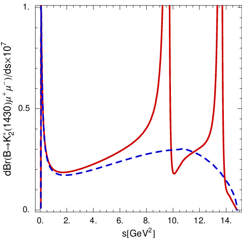
Figure 1: The differential decay rates d​Γtotal​(B0→K2∗0​(1430)​μ+​μ−)/d​sd\Gamma_{\rm total}(B^{0}\to K_{2}^{*0}(1430)\mu^{+}\mu^{-})/ds as functions of the dimuon invariant mass ss. The solid (dashed) curve corresponds to the center value of the decay rate with (without) the charmonium resonance effects.
Refer to caption

In Fig. 1, the total decay rates for B→K2∗​(1430)​μ+​μ−B\to K_{2}^{*}(1430)\mu^{+}\mu^{-}with and without charmonium resonances are plotted. The detailed results for the charmonium resonances can be found in Refs. [44, 45]. The branching fraction for nonresonant B→K2∗​μ+​μ−B\to K_{2}^{*}\mu^{+}\mu^{-} is obtained to be

ℬ⁡(B0→K2∗0​(1430)​μ+​μ−)\displaystyle{\cal B}(B^{0}\to K_{2}^{*0}(1430)\mu^{+}\mu^{-}) =\displaystyle= (3.5)−0.6+1.1−1.0+0.7×10⁻⁷,\displaystyle(3.5{}^{+1.1}_{-1.0}{}^{+0.7}_{-0.6})\times 10^{-7}, (60)

where the first error comes from the variation of ζ⟂\zeta_{\perp} in Eq. (44), the second error from the uncertainty of ξ\xi in Eq. (45).

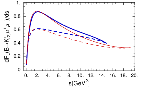
The longitudinal fraction distribution for B→K2∗​ℓ+​ℓ−B\to K_{2}^{*}\ell^{+}\ell^{-} decay is defined as

d​FLd​s≡d​ΓLd​s/d​Γtotald​s.\displaystyle\frac{dF_{L}}{ds}\equiv\frac{d\Gamma_{L}}{ds}\Bigg/{\frac{d\Gamma_{\rm total}}{ds}}. (61)

In Fig. 2, the longitudinal fraction distribution for the B→K2∗​(1430)​μ+​μ−B\to K_{2}^{*}(1430)\mu^{+}\mu^{-} decay is plotted. For comparison, we also plot FL​(B→K∗​(892)​μ+​μ−)/d​sF_{L}(B\to K^{*}(892)\mu^{+}\mu^{-})/ds as a benchmark. For small ss (≲3​GeV2\lesssim 3\,{\rm GeV}^{2}), B→K∗​μ+​μ−B\to K^{*}\mu^{+}\mu^{-} and B→K2∗​μ+​μ−B\to K_{2}^{*}\mu^{+}\mu^{-} have similar rates for the longitudinal fraction, while for large ss (≳4​GeV2\gtrsim 4\,{\rm GeV}^{2}) the d​FL/d​sdF_{L}/ds for the B→K2∗​μ+​μ−B\to K_{2}^{*}\mu^{+}\mu^{-} decay slightly exceeds the B→K∗​μ+​μ−B\to K^{*}\mu^{+}\mu^{-}. More interestingly, when s∼3​GeV2s\sim 3\,{\rm GeV}^{2}, the result of the new-physics models with the flipped sign solution for c7effc_{7}^{\rm eff} can deviate more remarkably from the SM prediction (and can be reduced by 20−3020-30%).

Figure 2: Longitudinal fraction distributions d​FL/d​sdF_{L}/ds as functions of ss. The thick (blue) and thin (red) curves correspond to the central values of B→K2∗0​(1430)​μ+​μ−B\to K_{2}^{*0}(1430)\mu^{+}\mu^{-} and B0→K∗0​(892)​μ+​μ−B^{0}\to K^{*0}(892)\mu^{+}\mu^{-} decays, respectively. The solid and dashed curves correspond to the SM and new-physics model with flipped sign of c7effc_{7}^{{\rm eff}}, respectively.
Refer to caption

The forward-backward asymmetry for the B¯→K¯2∗​ℓ+​ℓ−\overline{B}\to\overline{K}_{2}^{*}\ell^{+}\ell^{-} decay is given by

d​AFBd​s^\displaystyle\frac{dA_{\rm FB}}{d\hat{s}} =\displaystyle= −βT2​GF2​αE​M2​mB5210​π5​|Vt​s∗​Vt​b|2​s^​u^​(s)2​[Re⁡(ℬℰ∗)+Re⁡(𝒜ℱ∗)]|βT=1/2\displaystyle-\beta_{T}^{2}\frac{G_{F}^{2}\alpha_{EM}^{2}m_{B}^{5}}{2^{10}\pi^{5}}|V_{ts}^{*}V_{tb}|^{2}\hat{s}\hat{u}(s)^{2}\left[\mathop{\mbox{Re}}({\cal B}{\cal E}^{*})+\mathop{\mbox{Re}}({\cal A}{\cal F}^{*})\right]\biggr|_{\beta_{T}=\sqrt{1/2}} (62)
=\displaystyle= −βT2GF2​αE​M2​mB5210​π5|Vt​s∗Vt​b|2s^u^(s)2[Re(c10c9eff)VK2∗A1K2∗\displaystyle-\beta_{T}^{2}\frac{G_{F}^{2}\alpha_{EM}^{2}m_{B}^{5}}{2^{10}\pi^{5}}|V_{ts}^{*}V_{tb}|^{2}\hat{s}\hat{u}(s)^{2}\biggl[\mathop{\mbox{Re}}(c_{10}c_{9}^{{\rm eff}})V^{K_{2}^{*}}A_{1}^{K_{2}^{*}}
+m^bs^Re(c10c7eff){(1−m^K2∗)VK2∗T2K2∗+(1+m^K2∗)A1K2∗T1K2∗}]|βT=1/2.\displaystyle\phantom{M}+\frac{\hat{m}_{b}}{\hat{s}}\mathop{\mbox{Re}}(c_{10}c_{7}^{{\rm eff}})\left\{(1-\hat{m}_{K_{2}^{*}})V^{K_{2}^{*}}T_{2}^{K_{2}^{*}}+(1+\hat{m}_{K_{2}^{*}})A_{1}^{K_{2}^{*}}T_{1}^{K_{2}^{*}}\right\}\biggr]\biggr|_{\beta_{T}=\sqrt{1/2}}.

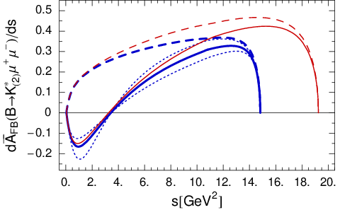
In Fig. 3 we illustrate the normalized forward-backward asymmetry d​A¯FB/d​s≡(d​AFB/d​s)/(d​Γtotal/d​s)d\overline{A}_{\rm FB}/ds\equiv(dA_{\rm FB}/ds)/(d\Gamma_{\rm total}/ds) for B→K2∗​μ+​μ−B\to K_{2}^{*}\mu^{+}\mu^{-} together with B→K∗​μ+​μ−B\to K^{*}\mu^{+}\mu^{-}.

In the SM, the forward-backward asymmetry zero s0s_{0} for B→K2∗​μ+​μ−B\to K_{2}^{*}\mu^{+}\mu^{-} is defined by

Re⁡[c10​c9eff​(s^0)]​VK2∗​(s0)​A1K2∗​(s0)\displaystyle\mathop{\mbox{Re}}[c_{10}c_{9}^{{\rm eff}}(\hat{s}_{0})]V^{K_{2}^{*}}(s_{0})A_{1}^{K_{2}^{*}}(s_{0}) (64)
=\displaystyle= −m^bs^0Re(c10c7eff){(1−m^K2∗)VK2∗(s0)T2K2∗(s0)+(1+m^K2∗)A1K2∗(s0)T1K2∗(s0)}.\displaystyle-\frac{\hat{m}_{b}}{\hat{s}_{0}}\mathop{\mbox{Re}}(c_{10}c_{7}^{{\rm eff}})\left\{(1-\hat{m}_{K_{2}^{*}})V^{K_{2}^{*}}(s_{0})T_{2}^{K_{2}^{*}}(s_{0})+(1+\hat{m}_{K_{2}^{*}})A_{1}^{K_{2}^{*}}(s_{0})T_{1}^{K_{2}^{*}}(s_{0})\right\}.

We obtain

s0\displaystyle s_{0} =\displaystyle= 3.4±0.1​GeV2,\displaystyle 3.4\pm 0.1\,{\rm GeV}^{2}, (65)

where the error comes from the variation of mbm_{b}. This result is very close to the zero for B→K∗​μ+​μ−B\to K^{*}\mu^{+}\mu^{-}. As shown in Fig. 3, it is interesting to note that the form factor uncertainty of the zero vanishes in the LEET limit.

The asymmetry zero exists only for Re⁡[c9eff​(s)​c10]​Re⁡(c7eff​c10)<0\mathop{\mbox{Re}}[c_{9}^{\rm eff}(s)c_{10}]\mathop{\mbox{Re}}(c_{7}^{\rm eff}c_{10})<0. Therefore with the flipped sign of c7effc_{7}^{\rm eff} along, compared with the SM prediction, the asymmetry zero disappears, and d​AFB/d​sdA_{\rm FB}/ds is positive for all values of ss. From recent measurements for B→K∗​ℓ+​ℓ−B\to K^{*}\ell^{+}\ell^{-} decays, the solution with the flipped sign of c7effc_{7}^{\rm eff} seems to be favored by the data [46, 22, 47]. One can find the further discussion in Ref. [26] for the B→K1​(1270)​ℓ+​ℓ−B\to K_{1}(1270)\ell^{+}\ell^{-} decays.

Figure 3: Forward-backward asymmetries d​A¯FB/d​sd\overline{A}_{\rm FB}/ds for B→K2∗​(1430)​μ+​μ−B\to K_{2}^{*}(1430)\mu^{+}\mu^{-}(thick curves) and B→K∗​(892)​μ+​μ−B\to K^{*}(892)\mu^{+}\mu^{-} (thin curves) as functions of the dimuon invariant mass ss. The solid and dashed curves correspond to the SM and new-physics model with flipped sign of c7effc_{7}^{\rm eff}. Variation due to the uncertainty from ζ∥​(q2)/ζ⟂​(q2)\zeta_{\parallel}(q^{2})/\zeta_{\perp}(q^{2}) (see Eq. (45)) is denoted by dotted curves.
Refer to caption

III.2 B→K2∗​ν​ν¯B\to K_{2}^{*}\nu\bar{\nu}

In the SM, b→s​ν​ν¯b\to s\nu\bar{\nu} proceeds through ZZ penguin and box diagrams involving top quark exchange [48]. One of the reasons that we are interested in the study of decays going through b→s​ν​ν¯b\to s\nu\bar{\nu} is the absence of long-distance corrections related to the relevant four-fermion operators. Moreover, the branching fractions are enhanced by the summation over three light neutrinos. New physics contributions arising from new loop and/or box diagrams may significantly modify the predictions. In the SM, the branching fractions involving KK or K∗K^{*} are predicted to be ℬ⁡(B→K​ν​ν¯)≃3.8×10⁻⁶{\cal B}(B\to K\nu\bar{\nu})\simeq 3.8\times 10^{-6} and ℬ⁡(B→K∗​ν​ν¯)≃13×10−6{\cal B}(B\to K^{*}\nu\bar{\nu})\simeq 13\times 10^{-6} [48, 49], while only upper limits 10−4∼10−510^{-4}\sim 10^{-5} were set in the experiments [13, 14, 22]. In the new physics scenario, the contribution originating from the nonstandard Z0Z^{0} coupling can enhance the branching fraction by a factor ten [32]. This mode is also relevant to search for light dark matter [33] and unparticles [34, 35].

The generally effective weak Hamiltonian relevant to the b→s​ν​ν¯b\to s\nu\bar{\nu} decay is given by

ℋeff=cL​s¯​γμ​(1−γ5)​b​ν¯​γμ​(1−γ5)​ν+cR​s¯​γμ​(1+γ5)​b​ν¯​γμ​(1−γ5)​ν,\displaystyle{\cal H}_{{\rm eff}}=c_{L}\bar{s}\gamma^{\mu}(1-\gamma_{5})b\,\bar{\nu}\gamma_{\mu}(1-\gamma_{5})\nu+c_{R}\bar{s}\gamma^{\mu}(1+\gamma_{5})b\,\bar{\nu}\gamma_{\mu}(1-\gamma_{5})\nu, (66)

where cLc_{L} and cRc_{R} are left- and right-handed weak hadronic current contributions, respectively. New physics effects can modify the SM value of cLc_{L}, while cRc_{R} only receives the contribution from physics beyond the SM [32]. In the SM we have

cLS​M\displaystyle c_{L}^{SM} =\displaystyle= GF2​αE​M2​π​sin2⁡θW​Vt​b​Vt​s∗​X​(xt)=2.9×10⁻⁹,\displaystyle\frac{G_{F}}{\sqrt{2}}\frac{\alpha_{EM}}{2\pi\sin^{2}\theta_{W}}V_{tb}V_{ts}^{*}X(x_{t})=2.9\times 10^{-9}, (67)

where the detailed form of X⁡(xt)X(x_{t}) can be found in Refs. [50, 51, 52, 53]. The K2∗K_{2}^{*} helicity polarization rates of the missing invariant mass-squared distribution d​Γh/d​sd\Gamma_{h}/ds of the B→K2∗​ν¯​νB\to K_{2}^{*}\bar{\nu}\nu decay are given by [54, 55, 56, 32],

d​Γ0d​s^\displaystyle\frac{d\Gamma_{0}}{d\hat{s}} =\displaystyle= 3​αL2​|p→|48​π3​|cL−cR|2mK2∗2\displaystyle 3\alpha_{L}^{2}\frac{|\vec{p}|}{48\pi^{3}}\frac{|c_{L}-c_{R}|^{2}}{m_{K_{2}^{*}}^{2}} (68)
×[(mB+mK2∗)​(mB​E−mK2∗2)​A1K2∗​(q2)−2​mB2mB+mK2∗​|p→|2​A2K2∗​(q2)]2,\displaystyle\phantom{iii}\times\left[(m_{B}+m_{K_{2}^{*}})(m_{B}E-m_{K_{2}^{*}}^{2})A_{1}^{K_{2}^{*}}(q^{2})-\frac{2m_{B}^{2}}{m_{B}+m_{K_{2}^{*}}}|\vec{p}|^{2}A_{2}^{K_{2}^{*}}(q^{2})\right]^{2},
d​Γ±1d​s^\displaystyle\frac{d\Gamma_{\pm 1}}{d\hat{s}} =\displaystyle= 3​βT2​|p→|​q248​π3\displaystyle 3\beta_{T}^{2}\frac{|\vec{p}|q^{2}}{48\pi^{3}} (69)
×|(cL+cR)​2​mB​|p→|mB+mK2∗​VK2∗​(q2)∓(cL−cR)​(mB+mK2∗)​A1K2∗​(q2)|2,\displaystyle\times\biggl|(c_{L}+c_{R})\frac{2m_{B}|\vec{p}|}{m_{B}+m_{K_{2}^{*}}}V^{K_{2}^{*}}(q^{2})\mp(c_{L}-c_{R})(m_{B}+m_{K_{2}^{*}})A_{1}^{K_{2}^{*}}(q^{2})\biggr|^{2},

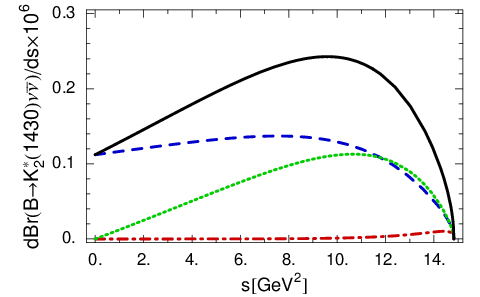
where s^≡s/mB2\hat{s}\equiv s/m_{B}^{2}, αL=2/3\alpha_{L}=\sqrt{2/3} and βT=1/2\beta_{T}=\sqrt{1/2} with 0≤s≤(mB−mK2∗)20\leq s\leq(m_{B}-m_{K_{2}^{*}})^{2} being the invariant mass squared of the neutrino-antineutrino pair. Here the factor 33 counts the numbers of the neutrino generations. p→\vec{p} and EE are the three-momentum and energy of the K2∗K_{2}^{*} in the BB rest frame. In Fig. 4, we show the distribution of the missing invariant mass-squared for the B→K2∗​(1430)​ν¯​νB\to K_{2}^{*}(1430)\bar{\nu}\nu decay within the SM.

Figure 4: Branching fraction distribution d​ℬ​(B0→K2∗0​ν¯​ν)/d​sd{\cal B}(B^{0}\to K_{2}^{*0}\bar{\nu}\nu)/ds as a function of the missing invariant mass squared ss within the SM. The solid (black), dashed (blue), dotted (green) and dot-dashed (red) curves correspond to the total decay rate and the polarization rates with helicities h=0h=0, −1-1, +1+1, respectively.
Refer to caption

We find

ℬ(B0→K2∗0(1430)ν¯ν)=(2.8−0.8+0.9)−0.5+0.6×10⁻⁶,\displaystyle{\cal B}(B^{0}\to K_{2}^{*0}(1430)\bar{\nu}\nu)=(2.8^{+0.9}_{-0.8}{}^{+0.6}_{-0.5})\times 10^{-6}, (70)

where the first and second errors are due to the uncertainty of the form factors and ξ\xi, respectively.

IV Summary

We have studied the radiative and semileptonic BB decays involving the tensor meson K2∗​(1430)K_{2}^{*}(1430) in the final states. Using the large energy effective theory techniques, B→K2∗​(1430)B\to K_{2}^{*}(1430) transition form factors have been formulated in the large recoil region. There are only two independent functions ζ⟂​(q2)\zeta_{\perp}(q^{2}) and ζ∥​(q2)\zeta_{\parallel}(q^{2}) that describe all relevant form factors. We have determined the value of ζ⟂​(0)\zeta_{\perp}(0) from the measurement of ℬ⁡(B0→K2∗0​(1430)​γ){\cal B}(B^{0}\to K_{2}^{*0}(1430)\gamma). Adopting a dipole q2q^{2}-dependency for the LEET functions and ζ∥​(q2)/ζ⟂​(q2)=1.0±0.2\zeta_{\parallel}(q^{2})/\zeta_{\perp}(q^{2})=1.0\pm 0.2, for which the former consists with the QCD counting rules and the latter is favored by the B→ϕ​K2∗B\to\phi K_{2}^{*} data, we have investigated the decays B→K2∗​ℓ+​ℓ−B\to K_{2}^{*}\ell^{+}\ell^{-} and B→K2∗​ν​ν¯B\to K_{2}^{*}\nu\bar{\nu}. Note that ζ∥\zeta_{\parallel} only gives corrections of order mK2∗/mBm_{K_{2}^{*}}/m_{B}. We have discussed two dedicated observables, the longitudinal distribution d​FL/d​sdF_{L}/ds and forward-backward asymmetry, in the B→K2∗​ℓ+​ℓ−B\to K_{2}^{*}\ell^{+}\ell^{-} decay. Recent forward-backward asymmetry measurements for B→K∗​ℓ+​ℓ−B\to K^{*}\ell^{+}\ell^{-} decays [3, 15, 11] seem to (i) allow the possibility of flipping the sign of c7effc_{7}^{{\rm eff}}, or (ii) have both c9c_{9} and c10c_{10} flipped in sign, as compared with the SM. Meanwhile, in the large recoil region, BABAR has recently reported the large isospin asymmetry for the B→K∗​ℓ+​ℓ−B\to K^{*}\ell^{+}\ell^{-} decays, which qualitatively favors the flipped sign c7effc_{7}^{{\rm eff}} model over the SM [22]. Therefore in the present study, in addition to the SM, we focus the new-physics effects on c7effc_{7}^{{\rm eff}} with the sign flipped. It should be note that the magnitude of c7effc_{7}^{{\rm eff}} is stringently constrained by the B→Xs​γB\to X_{s}\gamma data which is consistent with the SM prediction.

For the B→K2∗​ℓ+​ℓ−B\to K_{2}^{*}\ell^{+}\ell^{-} decay, of particular interest is the large recoil region, where the uncertainties of form factors are considerably reduced not only by taking the ratios of the form factors but also by computing in the large EK2∗E_{K_{2}^{*}} limit. In this region, where the invariant mass of the lepton pair s≃2−4​GeV2s\simeq 2-4\,{\rm GeV}^{2}, due to the flipped sign of c7effc_{7}^{{\rm eff}} compared with the SM result, d​FL/d​sdF_{L}/ds is reduced by 20−3020-30%, and its value can be ∼0.8\sim 0.8. One the other hand, in the SM the asymmetry zero is about 3.4​GeV23.4\,{\rm GeV}^{2}, but changing the sign of c7effc_{7}^{{\rm eff}} yields a positive forward-backward asymmetry for all values of the invariant mass of the lepton pair.

We have obtained the branching fraction for B→K2∗​ν​ν¯B\to K_{2}^{*}\nu\bar{\nu} in the SM. This mode enhanced by the summation over three light neutrinos is theoretically cleaner due to the absence of long-distance corrections related to the relevant four-fermion operators. This decay is relevant for the search for the nonstandard Z0Z^{0} coupling, light dark matter and unparticles.

In summary, the investigation of the semileptonic BB decays involving K2∗​(1430)K_{2}^{*}(1430) will further provide complementary information on physics beyond the standard model. Our results also exhibit the impressed resemblance of the physical properties between B→K2∗​(1430)​ℓ+​ℓ−,ν​ν¯B\to K_{2}^{*}(1430)\ell^{+}\ell^{-},\nu\bar{\nu} and B→K∗​(892)​ℓ+​ℓ−,ν​ν¯B\to K^{*}(892)\ell^{+}\ell^{-},\nu\bar{\nu}.

Acknowledgements.
This research was supported in parts by the National Science Council of R.O.C. under Grant No. NSC96-2112-M-033-004-MY3 and No. NSC97-2811-033-003 and by the National Center for Theoretical Science.

References

  • [1] I. Adachi et al. [Belle Collaboration], arXiv:0810.0335 [hep-ex].
  • [2] B. Aubert et al. [BABAR Collaboration], Phys. Rev. Lett. 102, 091803 (2009) arXiv:0807.4119 [hep-ex].
  • [3] A. Ishikawa et al., Phys. Rev. Lett. 96, 251801 (2006) [arXiv:hep-ex/0603018].
  • [4] E. Barberio et al. [Heavy Flavor Averaging Group], arXiv:0808.1297 [hep-ex].
  • [5] A. Yarritu et al. [BABAR Collaboration], arXiv:0808.1915 [hep-ex].
  • [6] M. Nakao et al. [BELLE Collaboration], Phys. Rev. D 69, 112001 (2004) [arXiv:hep-ex/0402042].
  • [7] T. E. Coan et al. [CLEO Collaboration], Phys. Rev. Lett. 84, 5283 (2000) [arXiv:hep-ex/9912057].
  • [8] B. Aubert et al. [BABAR Collaboration], Phys. Rev. D 70, 091105 (2004) [arXiv:hep-ex/0409035].
  • [9] S. Nishida et al. [Belle Collaboration], Phys. Rev. Lett. 89, 231801 (2002) [arXiv:hep-ex/0205025].
  • [10] B. Aubert et al. [BABAR Collaboration], Phys. Rev. D 73, 092001 (2006) [arXiv:hep-ex/0604007].
  • [11] I. Adachi [The Belle Collaboration], arXiv:0810.0335 [hep-ex].
  • [12] S. Anderson et al. [CLEO Collaboration], Phys. Rev. Lett. 87, 181803 (2001) [arXiv:hep-ex/0106060].
  • [13] K. F. Chen et al. [BELLE Collaboration], Phys. Rev. Lett. 99, 221802 (2007) [arXiv:0707.0138 [hep-ex]].
  • [14] B. Aubert et al. [BABAR Collaboration], Phys. Rev. D 78, 072007 (2008) [arXiv:0808.1338 [hep-ex]].
  • [15] B. Aubert et al. [BABAR Collaboration], arXiv:0804.4412 [hep-ex].
  • [16] W. J. Li, Y. B. Dai and C. S. Huang, Eur. Phys. J. C 40, 565 (2005) [arXiv:hep-ph/0410317].
  • [17] G. Burdman, Phys. Rev. D 52, 6400 (1995) [arXiv:hep-ph/9505352].
  • [18] J. L. Hewett and J. D. Wells, Phys. Rev. D 55, 5549 (1997) [arXiv:hep-ph/9610323].
  • [19] Y. G. Xu, R. M. Wang and Y. D. Yang, Phys. Rev. D 74, 114019 (2006) [arXiv:hep-ph/0610338].
  • [20] P. Colangelo, F. De Fazio, R. Ferrandes and T. N. Pham, Phys. Rev. D 73, 115006 (2006) [arXiv:hep-ph/0604029].
  • [21] C. H. Chen and C. Q. Geng, Phys. Rev. D 66, 094018 (2002) [arXiv:hep-ph/0209352].
  • [22] G. Eigen, arXiv:0807.4076 [hep-ex].
  • [23] T. Feldmann and J. Matias, JHEP 0301, 074 (2003) [arXiv:hep-ph/0212158].
  • [24] A. Ali, P. Ball, L. T. Handoko and G. Hiller, Phys. Rev. D 61, 074024 (2000) [arXiv:hep-ph/9910221].
  • [25] H. Hatanaka and K. C. Yang, Phys. Rev. D 77, 094023 (2008) [Erratum-ibid. D 78, 059902 (2008)] [arXiv:0804.3198 [hep-ph]].
  • [26] H. Hatanaka and K. C. Yang, Phys. Rev. D 78, 074007 (2008) [arXiv:0808.3731 [hep-ph]].
  • [27] H. Yang et al., Phys. Rev. Lett. 94, 111802 (2005) [arXiv:hep-ex/0412039].
  • [28] H. Y. Cheng and C. K. Chua, Phys. Rev. D 69, 094007 (2004) [arXiv:hep-ph/0401141].
  • [29] D. Ebert, R. N. Faustov and V. O. Galkin, Phys. Rev. D 64, 094022 (2001) [arXiv:hep-ph/0107065]; D. Ebert, R. N. Faustov, V. O. Galkin and H. Toki, Phys. Rev. D 64, 054001 (2001) [arXiv:hep-ph/0104264].
  • [30] A. Datta, Y. Gao, A. V. Gritsan, D. London, M. Nagashima and A. Szynkman, Phys. Rev. D 77, 114025 (2008) [arXiv:0711.2107 [hep-ph]].
  • [31] J. Charles, A. Le Yaouanc, L. Oliver, O. Pene and J. C. Raynal, Phys. Rev. D 60, 014001 (1999) [arXiv:hep-ph/9812358].
  • [32] G. Buchalla, G. Hiller and G. Isidori, Phys. Rev. D 63, 014015 (2000) [arXiv:hep-ph/0006136].
  • [33] C. Bird, P. Jackson, R. V. Kowalewski and M. Pospelov, Phys. Rev. Lett. 93, 201803 (2004) [arXiv:hep-ph/0401195].
  • [34] H. Georgi, Phys. Rev. Lett. 98, 221601 (2007) [arXiv:hep-ph/0703260].
  • [35] T. M. Aliev, A. S. Cornell and N. Gaur, JHEP 0707, 072 (2007) [arXiv:0705.4542 [hep-ph]].
  • [36] E. R. Berger, A. Donnachie, H. G. Dosch and O. Nachtmann, Eur. Phys. J. C 14, 673 (2000) [arXiv:hep-ph/0001270].
  • [37] C. Amsler et al. [Particle Data Group], Phys. Lett. B 667, 1 (2008).
  • [38] CKMfitter Group (http://ckmfitter.in2p3.fr), results as of 2008 summer.
  • [39] M. Beneke, T. Feldmann and D. Seidel, Nucl. Phys. B 612, 25 (2001) [arXiv:hep-ph/0106067].
  • [40] A. Ali and A. Y. Parkhomenko, Eur. Phys. J. C 23, 89 (2002) [arXiv:hep-ph/0105302].
  • [41] S. W. Bosch and G. Buchalla, Nucl. Phys. B 621, 459 (2002) [arXiv:hep-ph/0106081].
  • [42] V. L. Chernyak and A. R. Zhitnitsky, Phys. Rept. 112, 173 (1984).
  • [43] Heavy Flavor Averaging Group, E. Barberio et al., arXiv:0704.3575 [hep-ex] and online update at http://www.slac.stanford.edu/xorg/hfag.
  • [44] C. S. Lim, T. Morozumi and A. I. Sanda, Phys. Lett. B 218, 343 (1989).
  • [45] A. Ali, T. Mannel and T. Morozumi, Phys. Lett. B 273, 505 (1991).
  • [46] J. Matias, Nucl. Phys. Proc. Suppl. 185, 68 (2008) [arXiv:0807.2579 [hep-ph]].
  • [47] C. Bobeth, G. Hiller and G. Piranishvili, JHEP 0807, 106 (2008) [arXiv:0805.2525 [hep-ph]].
  • [48] A. J. Buras and R. Fleischer, Adv. Ser. Direct. High Energy Phys. 15, 65 (1998) [arXiv:hep-ph/9704376].
  • [49] A. Ali and T. Mannel, Phys. Lett. B 264, 447 (1991) [Erratum-ibid. B 274, 526 (1992)].
  • [50] T. Inami and C. S. Lim, Prog. Theor. Phys. 65, 297 (1981) [Erratum-ibid. 65, 1772 (1981)].
  • [51] G. Buchalla and A. J. Buras, Nucl. Phys. B 400, 225 (1993).
  • [52] G. Buchalla, A. J. Buras and M. E. Lautenbacher, Rev. Mod. Phys. 68, 1125 (1996) [arXiv:hep-ph/9512380].
  • [53] G. Buchalla and A. J. Buras, Nucl. Phys. B 548, 309 (1999) [arXiv:hep-ph/9901288].
  • [54] P. Colangelo, F. De Fazio, P. Santorelli and E. Scrimieri, Phys. Lett. B 395, 339 (1997) [arXiv:hep-ph/9610297].
  • [55] D. Melikhov, N. Nikitin and S. Simula, Phys. Lett. B 428, 171 (1998) [arXiv:hep-ph/9803269].
  • [56] C. S. Kim, Y. G. Kim and T. Morozumi, Phys. Rev. D 60, 094007 (1999) [arXiv:hep-ph/9905528].