Discontinuities of plane functions projected from a surface with methods for finding these

A function $f:{\bf\mathbb{R}}^{m}\rightarrow{\bf\mathbb{R}}$ is continuous at $x\in\mathbb{R}^{m}$ if for every sequence $x_{i}$ converging to $x$, the sequence $f(x_{i})$ converges to $f(x)$. Thus any subsequence of any sequence $f(x_{i})$ converges to the same limit, namely $f(x)$.

Unfortunately, the definition of continuity is not helpful as to how we may locate a discontinuity in an image, which is a finite array of measurements. This paper presents a mathematical result which enables one to find points where a function $I:\mathbb{R}^{2}\rightarrow\mathbb{R}$ is not smooth, such as discontinuities. It is assumed that $I$ is induced by a smooth mapping

In previous work [11] a problem which arose in computer vision was formulated using the shape spaces introduced by Kendall. An application of the explicit solution was the following. An image is acquired from a video camera. The image contains a shape such as a triangle, square or circle. The problem is to classify it into categories such as triangles, squares or circles. For example, an image of a triangle will typically contain far more than three points, so it needs to be simplified. A square on the other hand should not be simplified to a triangle, and a circle should not be simplified very much at all. In order to obtain the points to be simplified in the first place, we first have to find discontinuities in $I$.

This paper is concerned with the mathematical aspects of the discontinuity identification problem. In what follows it is assumed the reader is familiar with differential geometry. Although the result is motivated by computer vision and human vision, differential geometry is not familiar there. As a mathematical result it could be extended by a wider scientific audience by replacing the above $\iota$ with some other measurement $\iota$.

It is very surprising that using optical principles, we can establish mathematically that there really is a discontinuity. Not some other property such as a local maximum in a derivative, but a discontinuity. The derivative is defined in calculus or real analysis. All books on real analysis [2] make it clear that continuity is a necessary condition for the derivative to be well-defined.

When grappling with this problem others have used piecewise smooth or other assumptions. Instead here the contrapositive will be used to obtain a more general result. Owing to the microstructure of a scene surface, the light radiated from the surface undergoes extremely rapid intensity changes over small regions. This can be confirmed by examining gray values of neighbouring points in a real image. It is for this reason that this more general result may be helpful.

A fundamental psychological observation about the nature of vision was made by Wertheimer, who noticed the apparent motion not of individual dots, but of fields in images presented sequentially as a movie [16]. This started the Gestalt school of psychology [17, 10].

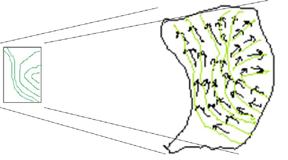
A differential operator maps a greyscale image to a vector field. It is implicitly suggested by Hoffman [8] that the primary visual cortex of the brain produces some sort of vector field. It should be possible to line up the vectors in a head to tail fashion to form contours. We want to know when this results in a family of closed oriented contours rather like a topographic map. The answer is provided by a famous theorem of differential geometry, namely the Foliation theorem of Frobenius.

In what follows we consider a real valued function on the plane. Some examples of such functions in a color image are red, blue, green, hue, saturation or brightness.

It is an example of what is called a one dimensional distribution in differential geometry [14], [3]. The vector field is called a basis for this distribution.

Thus an integral curve is a curve whose tangent at each point coincides with the vector of the vector field at the same point. Since the gradient vector points in the direction of steepest descent, perpendicular vectors are produced by the Hamiltonian operator, and if we join these Hamiltonian vectors in a head to tail fashion, they line up into integral curves.

The following is the authors Theorem 3.3 from [1].

Then

Thus $d\iota(v)\mid_{a}=0$ if and only if $v$ is a multiple of $a$. Thus $d\iota(v)$ has rank $2$ at all points on a surface disjoint from the focal plane, except occluding points, where it has rank $1$.

The corollaries to the theorem 6 give us a condition to establish that there is a discontinuity or occlusion in an image.

The contrapositive is often used in mathematics, mainly for proofs by contradiction, such as the irrationality of the square root of two. Consider any predicates $P,\>Q$ and denote $notP$ and $notQ$ by $\neg P,\neg Q$. The contrapositive of $P$$\Rightarrow Q$ is $\neg Q\Rightarrow\neg P$. Since $P\Rightarrow Q$ is $\neg P$$\vee Q$ then $\neg(\neg P)$$\vee\neg Q$ which is $P\vee\neg Q$ thus $\neg Q\Rightarrow\neg P$. It is the contrapositive that enables us to find a discontinuity.

In other words, we have obtained a sufficient condition for a singularity in intensity, or the surface or an occlusion.

The following lemma gives us a means for finding integral curves in closed form. Its relevance to vision was observed by Faugeras (see pg112 of [6]); those image curves whose normals are parallel to the gradient are the level curves of intensity. What follows is an alternate statement.

Thus the Hamiltonian is an operator whose integral curves we can calculate in closed form, circumventing all the errors associated with numerical differentiation, numerical equation solving, and even floating point arithmetic. However there is an exception at a finite number of points where the vector field on a surface vanishes.

An image is only a discrete sample of measurements of light reflected from a surface. If a pixel has a particular measurement value, none of its neighbors necessarily has the same value. It is therefore not feasible to calculate level curves by trying to chain together pixels that have the same measurement value. A more sensible procedure is to calculate the set of image points whose measurement value is less than the particular measurement value, and then compute the boundary of this set (Figure 3).

The surfaces of objects in scenes have another property, namely they are bounded, and can be considered to be closed sets. A closed and bounded subset of ${\bf\mathbb{R}}^{m}$ is called compact. A more general definition of compactness can be given in the more general setting of topological spaces. A collection of open sets is said to cover a set $S$ if $S$ is contained in the union of all the open sets in the collection. A set $S$ is called compact if every collection of open sets covering $S$ has a finite sub-collection that covers $S$. This is not an easy property to grasp, but it is a very important one. Theorem 6.3 in [13] asserts that the closed and bounded subsets of ${\bf\mathbb{R}}^{m}$ coincide with the compact subsets.

Surfaces can therefore be considered to be compact manifolds, but this includes parts of the surface that are not visible, or in contact with other surfaces like the ground.

It can be shown that all maximal integral curves of a compact smooth manifold are complete [14]. Thus a hypothesis that an image is a smooth image of an unoccluded, smooth compact surface implies that all maximal integral curves are closed curves. We intuitively know that this follows from an absurd assumption, namely that all of a surface is visible. However, since we want to reject such a hypothesis, we must employ the consequences which are most certain to lead to a contradiction. This is why we will generate only closed curves, by completion of curves if necessary. The phenomenon of completion occurs in human vision, and can be demonstrated vividly by an optical illusion called the Kanisza triangle.

An algorithm was implemented based on Theorem 12, using values $c$ in constant increments. This algorithm used no floating point arithmetic. This was run on a super-computer belonging to the University of Melbourne. The results of this were surprising. If very small increments are chosen then almost the entire image is returned. What this shows is that the algorithm can detect discontinuities that are dense, not just discontinuities that fall on a curve. However if larger increments are chosen, then edges are returned. The discontinuities found do not surround objects completely.

We will now show that the existence of a neighboring point and a threshold such that the difference in measurements exceeds the threshold is a necessary but not sufficient condition for an occlusion or singularity to exist.

We have shown that if the sufficient condition for an occlusion or discontinuity in an image or scene is met at a point in an image (see Theorem 3.3 in PhD thesis), then there is a neighboring point and a threshold that must be exceeded. In other words we have obtained a necessary condition for a sufficient condition. Unfortunately this does not suffice because the condition is not necessary and sufficient.

What this lemma and example tells us is that threshold’s will give us a set of occlusions and discontinuities, but will also include points that are neither occlusions nor discontinuities. We now give a stronger condition that is more useful.

Suppose $p\in I_{c}\cap I_{c^{\prime}}$ with $c\neq c^{\prime}$. Then

and

Letting $\varepsilon=c-I\left(p_{c}\right)$ and $\varepsilon^{\prime}=c^{\prime}-I\left(p_{c^{\prime}}\right)$ and $p^{\prime}=p_{c}$ and $p^{\prime\prime}=p_{c^{\prime}}$ it follows that $I\left(p\right)-I\left(p^{\prime}\right)\geq\varepsilon>0$ and $I\left(p\right)-I\left(p^{\prime\prime}\right)\geq\varepsilon^{\prime}>0$.

The reader should note that the neighboring points $p^{\prime}$ and $p^{\prime\prime}$ can coincide, providing $\varepsilon\neq\varepsilon^{\prime}$

Consider $H=\left(-\frac{\partial}{\partial t},\frac{\partial}{\partial x}\right)$ which is a Hamiltonian operator. The integral curves of $H$ are level curves $I\left(x,t\right)$.

The lemma shows that if $\left(x,t\right)$ has two neighboring points $\left(x_{i},t_{i}\right)i=1,2$ such that $I\left(x,t\right)-I\left(x_{i},t_{i}\right)>\varepsilon_{i}>0$ with $\varepsilon_{1}+I\left(x_{1},t_{1}\right)\neq\varepsilon_{2}+I\left(x_{2},t_{2}\right)$ then there is an occlusion or discontinuity at$\left(x,t\right)$.

So if we used two consecutive video frames and two different thresholds, we could apply the test to the time increments to determine a set of occlusions and discontinuities. We could also use three consecutive video frames and two different thresholds, and apply the test.

Note that we can apply any smooth differential operator to the image function. For example we could differentiate the green component and set $I\left(x,y\right)=\left(\frac{\partial G}{\partial x}\right)\left(x,y\right)$. Then applying the same algorithm to I would determine a set of occlusions and discontinuities. We can also use higher order smooth differential operators, or finite difference approximations to smooth differential operators. In fact we can use absolutely any process that transforms an arbitrary smooth function into another arbitrary smooth function, to substitute in a new I into the algorithm.

Two main components of a camera or the eye are a lens and a collection of light sensors on a surface, called the retina. The retina of a camera is usually planar, and will be referred to as the retinal plane. The camera forms an image of the scene in front of it. The correspondence between a point in the scene and a point in the retinal plane can be approximately given by a straight line through the optical centre of the camera (see figure 5 ).

This model can be justified by geometric optics. A convex lens with two spherical surfaces whose thickness can be neglected is called a thin lens in geometric optics. The lens of a camera is usually a series of thin lenses (called a thick lens in geometric optics, see page 25 of [15]). The paraxial or Gaussian assumption of geometric optics is that the angle between a scene point and the optical axis of the lens system is small. It is known in geometric optics that, under the paraxial assumption, the vertical distance between the scene point and the optical axis and the vertical distance between its focussed image point and the optical axis is a constant, called the magnification of the lens system (see page 28 of [15]).

The elementary physical concept of reflection is that a light ray incident to a surface will be reflected at an angle to the surface normal equal to the angle of incidence, such that incident and exitant rays lie in the same plane through the normal vector. A mirror is an example of such an ideal, or specular reflector. The microscopic structure of most materials in scenes is not smooth, so a scene surface will scatter light in different directions. Most materials are also not perfectly homogeneous on a microscopic scale, and thus scatter light rays that penetrate the surface by refraction and reflection at boundaries between regions of different refractive indices. Scattered rays may reemerge near the point of entry, and so contribute to diffuse reflection. Snow and layers of white paint are examples of materials with this behaviour [9].

A surface is called Lambertian if it appears equally bright from all directions, regardless of how it is irradiated, and reflects all incident light [9]. This does not imply that different points on the same surface have the same intensity, because the value of the intensity depends on other variables such as the angle between the surface normal and a light source. When a smooth lambertian surface is rendered by computer graphics, its appearance is like a dull smooth plastic [12].

Most materials in scenes are neither specular reflectors nor Lambertian reflectors, but a combination of both. A surface rendered by computer graphics will appear shinier as the specular component is increased [12, 7]. The appearance of texture (to the eye) is due to particularly rapid variations in normal vectors over small regions. For example, a random pattern of normal vectors when rendered by computer graphics can produce an effect of fog. Various repetitive patterns of normal vectors can be used to render real materials, such as bricks by computer graphics [7]. The Lambertian assumption can also be used to directly recover surface shape from image shading [4, 5].

Owing to the microstructure of a scene surface, the light radiated from the surface undergoes extremely rapid intensity changes over small regions. This can be confirmed by examining gray values of neighbouring points in a real image.

Let $\iota:(x,y,z)\rightarrow(t,s)$ where $t=\frac{x}{z},\,s=\frac{y}{z}$, and $z\neq 0$. For a camera with retina at $z=1$ and optical centre at the origin, the function $\iota$ represents image formation. The point $(x,y,z)$ is being viewed, and its image is formed at $(\frac{x}{z},\frac{y}{z})$.

Note that the co-ordinates $(t,s)$ must be $(0,0)$ at the point where the optical axis meets the retinal plane perpendicularly. It is preferred to find this point in the image by some procedure. Zooming the camera and finding the point around which the image expands or contracts may be one way. The unit of distance is approximately the distance between the pupil and the ccd.

For the purpose of stereo or binocular vision, points in an image where the surface being viewed is not smooth need to be distinguished from occluding points. This is because under the assumption of Lambertian shading, different viewpoints of the same point have similar intensity values. Points where the surface being viewed is not smooth possess invariance to viewpoint. On the other hand occluding points move on the surface when they are viewed from a different viewpoint. Occluding points can be eliminated by filtering out zeroes of the Hamiltonian. This does require floating point arithmetic. For other purposes such as robot navigation where we are just looking for empty spaces this is not an issue.

Also note that we could use any discrete topology on the plane to define the neighbors of a point. For example we could use 4 neighbors north, west, east and south of each pixel. Or we could use 8 neighbors. Or some other topology would also do.

References

- [1] B. Bhavnagri. Computer Vision using Shape Spaces. PhD thesis, University of Adelaide, 1996.
- [2] K.G. Binmore. Mathematical analysis: a straightforward approach. Cambridge University Press, 1982.
- [3] F. Brickell and R.S. Clark. Differentiable manifolds: an introduction. Van Nostrand Reinhold, 1970.
- [4] M.J. Brooks and W. Chojnacki. Direct computation of shape from shading. Pattern Recognition, 1:114–119, 1994.
- [5] W. Chojnacki, M.J. Brooks, and D. Gibbons. Revisiting pentlands estimator of light source direction. Journal of the Optical Society of America A, 11(1):118–124, 1994.
- [6] O. Faugeras. Three dimensional computer vision: a geometric viewpoint. MIT Press, 1993.
- [7] D. Hearn and M.P. Baker. Computer Graphics. Prentice-Hall, 1986.
- [8] W.C. Hoffman. The lie algebra of visual perception. Journal of Mathematical Psychology, 3(1):65–98, 1966.
- [9] B.K.P. Horn and R.W. Sjoberg. Calculating the reflectance map. In B.K.P. Horn and M.J. Brooks, editors, Shape from shading, chapter 8, pages 215–244. MIT Press, 1989.
- [10] G. Kanizsa. Organization in vision, essays on gestalt perception. Praeger, 1979.
- [11] H. Le and B. Bhavnagri. On simplifying shapes by subjecting them to collinearity constraints. Mathematical Proceedings of the Cambridge Philosophical Society, 121(2), 1997.
- [12] G. Lorig. Advanced image synthesis - shading. In Advances in computer graphics I, volume XII of Eurographic seminars, pages 441–456. Springer-Verlag, 1986.
- [13] J.R. Munkres. Topology: A first course. Prentice-Hall, Englewood Cliffs New Jersey, 1975.
- [14] F. W. Warner. Foundations of differential manifolds and lie groups. Springer-Verlag, New York, 1983.
- [15] W.T. Welford. Optics. Oxford Physics Series. Oxford Science Publications, 1988.
- [16] M. Wertheimer. Experimentelle studien uber das sehen von bewegung. Zeitschrift f. Psychol., 61:161–265, 1912.
- [17] M. Wertheimer. Laws of organization in perceptual forms. Harcourtm Brace and Co, 1938.