Flavor Superconductivity from Gauge/Gravity Duality
Abstract:
We give a detailed account and extensions of a holographic flavor superconductivity model which we have proposed recently. The model has an explicit field theory realization as strongly coupled Super Yang-Mills theory with fundamental matter at finite temperature and finite isospin chemical potential. Using gauge/gravity duality, i. e. a probe of two flavor D7–branes in the AdS black hole background, we show that the system undergoes a second order phase transition with critical exponent 1/2. The new ground state may be interpreted as a meson superfluid. It shows signatures known from superconductivity, such as an infinite dc conductivity and a gap in the frequency-dependent conductivity. We present a stringy picture of the condensation mechanism in terms of a recombination of strings. We give a detailed account of the evaluation of the non-Abelian Dirac-Born-Infeld action involved using two different methods. Finally we also consider the case of massive flavors and discuss the holographic Meissner–Ochsenfeld effect in our scenario.
Keywords:
Gauge-gravity correspondence, D-branes, Black Holes1 Introduction and summary
Gauge/gravity duality has been used very successfully over the past years to obtain models with properties very similar to experimentally observed phenomena in both elementary and condensed matter physics. This is due to the fact that gauge/gravity duality is a powerful tool to compute observables of field theories at strong coupling [1]. In view of applications, it is particularly useful to turn on a temperature using an AdS black hole as gravity dual, as first proposed in [2]. In particular, gauge/gravity duality models which exhibit properties known from superconductivity have recently been constructed [3, 4, 5, 6, 7, 8, 9, 10, 11, 12, 13, 14, 15, 16, 17, 18, 19, 20, 21, 22].
In this context we have recently proposed a model which represents a stringy realization of superconductivity in a relativistic framework [14]. The aim of the present paper is to give a detailed account of the setup and calculations involved in obtaining the results of [14], as well as further new results.
Our model is based on embedding a probe of two coincident D7 branes into the AdS-black hole background, which extends the original correspondence to a field theory with flavor degrees of freedom in the fundamental representation of the gauge group, along the lines of [23, 24, 25]. Using this approach, the correspondence has also been applied to finite flavor charge densities [26, 27, 28, 29, 30, 31, 32]. A finite charge density for the flavor symmetry is obtained by giving a vev to the time component of the gauge field on the D7 brane probe. In [32], a finite isospin density was considered using a probe of two coincident D7 branes and switching on a gauge field on the probe. At high isospin densities , this configuration becomes unstable against gauge field fluctuations and , corresponding to vector mesons [33] in the field theory (see Figure 1) (see [34] for an early discussion of a similar instability). Note that we use capital letters for the background and small letters for the fluctuations.

The central result obtained in this model [14] is that there is a solution to the equation of motion for the field on the two flavor branes, which in addition to the finite isospin density has a further vev of the form . This solution has lower free energy in the new phase shown in figure 1 and stabilizes this phase. This applies at least to stability against the fluctuations and . Moreover we find that this phase has properties of a superconductor, such as a second order phase transition with a critical exponent of 1/2. The flavor current, which is analogous to the electromagnetic current, displays infinite dc conductivity and a gap in the frequency-dependent conductivity. Furthermore, there is a dual string-theoretical picture of the Cooper pairs, as well as dynamical generation of meson masses.
The stabilization mechanism encountered in this context is related to the results of [35]. Within the Sakai-Sugimoto model, a vev of the form was considered in [36] in the context of meson condensation. To obtain a p-wave superconductor within a phenomenological AdS/QCD model, a vev of the form was first used in [7]. Note that in our model the equations of motion forbid a source term for i. e. the breaking of the is spontaneous.
The results presented here can be interpreted in two different ways. On the one hand, our results provide an important link between gauge/gravity with flavor and the recent gauge/gravity realizations of superconducting states e. g. in [7, 3, 13], as well as a realization of a superconducting current from a top-down (super-)gravity model, rather than in a phenomenological bottom-up AdS/QCD model. Moreover, the degrees of freedom in the dual field theory are identified explicitly.
On the other hand, our holographic description can also be considered as a realization of a meson superfluid. In the model presented here, the mesons form a superfluid. In QCD like theories, meson condensation is discussed in [37, 38]. The corresponding picture is that the mesons move through the quark-gluon plasma without friction. Similarly, the absorption rate for radiation should be reduced for a specific frequency range [39]. For pions, similar results have been found within QCD: There are analytical results for small and very large isospin chemical potential using the chiral Lagrangian [40, 41], as well as lattice results [42]. Unlike the lattice results, the results presented here can easily be generalized to finite baryon chemical potential. A pion superfluid was obtained within gauge/gravity duality in [18].
Let us compare our results to QCD. In QCD, the pion condensate is of course the natural state in isospin asymmetric matter. The condensation of a particle sets in if the isospin chemical potential is larger than the mass of this particle. According to this rule, the pions condense first in QCD since they are the Nambu-Goldstone bosons of the spontaneous chiral symmetry breaking and therefore the lightest particles. However the dual field theory which we consider in this letter is supersymmetric at zero temperature and therefore chiral symmetry cannot be broken spontaneously. In this supersymmetric theory, the vector and scalar mesons have the same mass at zero temperature. Due to finite temperature effects, the mass of the vector and scalar mesons can become different as we increase the temperature. It is a priori unclear which particle will condense. In our model we checked that the vector mesons condense first such that the -meson condensation state, which we consider in this paper, is the physical ground state of our system near the phase transition.
In this paper we explain in detail the method used for evaluating the non-Abelian Dirac-Born-Infeld action involved. Moreover we give a detailed account of our results for finite quark mass and the derivation of the Meissner effect. Results similar to ours have also been obtained in [15] shortly after [14]. However there the non-abelian DBI action is considered only to second order in . Some of the features discussed here are also present in [15]: a second order phase transition as well as a gap in the frequency-dependent conductivity. However, since higher order terms in are not taken into account in [15], these authors are not able to see higher order excitations in the frequency-dependent conductivity. Here we identify these higher order peaks with meson resonances.
Moreover, we give a string-theoretical interpretation of the formation of a superconducting state of lower free energy: Essentially the condensation process corresponds to a recombination of strings. The detailed picture is as follows: A small isospin density corresponds to strings stretching from the D7 branes to the horizon [26], the horizon strings. These are located close to the horizon. Increasing the isospin density, the horizon strings strongly charge one of the D7 branes positively near the horizon, and the other negatively. At a critical value, it becomes energetically favorable for the horizon strings to recombine into D7-D7 strings which are free to move into the bulk and therefore lower the charge density near the horizon. The D7-D7 strings form the superconducting condensate. Thus they provide a picture of strongly coupled holographic Cooper pairs. Note that for the construction considered the non-Abelian structure generated by the two D-branes is essential since it provides a charged condensate. The non-Abelian forces play an important role for stabilizing the condensate.
This paper is organized as follows: We begin with describing the field-theory action in section 2. We then explain the dual supergravity setup in section 3. In particular, we contrast and compare two different approaches to evaluating the non-Abelian DBI action involved. These are an adapted symmetrized trace prescription and the expansion of the DBI action to fourth order. We frequently refer to these approaches as prescriptions. We then explain the string-theoretical picture in detail in section 4. Then we describe the thermodynamics of the phase transition in 5, and in particular show that it is second order with critical exponent 1/2. In 6 we evaluate the fluctuations, again in the two different approaches for the non-abelian DBI action. We calculate the frequency-dependent conductivity and show it displays the expected gap. Moreover we check that while the normal phase was unstable with respect to the fluctuations in and , the superconducting phase is now stable with respect to these fluctuations. Finally we show in 7 that our system displays a Meissner-Ochsenfeld effect. We conclude with a collection of remarks and suggestions in 8.
2 Field Theory Interpretation
In this paper we will focus on a 3+1 – dimensional supersymmetric Yang-Mills theory at temperature , consisting of a gauge multiplet as well as massive supersymmetric hypermultiplets The hypermultiplets give rise to the flavor degrees transforming in the fundamental representation of the gauge group. The action is written down explicitly for instance in [43]. In particular, we work in the large limit with at strong coupling, i. e. with where is the ’t Hooft coupling constant. In the following we will consider only two flavors, i. e. The flavor degrees of freedom are called and . If the masses of the two flavor degrees are degenerate, the theory has a global flavor symmetry, whose overall subgroup can be identified with the baryon number.
In the following we will consider the theory at finite isospin chemical potential , which is introduced as the source of the operator
| (1) |
where is the charge density of the isospin fields, and . are the Pauli matrices. A non-zero vev introduces an isospin density as discussed in [32]. The isospin chemical potential explicitly breaks the flavor symmetry down to , where is generated by the unbroken generator of the . Under the symmetry the fields with index and have positive and negative charge, respectively.
However, the theory is unstable at large isospin chemical potential [32]. The new phase is sketched in figure 1. We show in this paper (see also [14]), that the new phase is stabilized by a non–vanishing vacuum expectation value of the current component
| (2) |
This current component breaks both the rotational symmetry as well as the remaining Abelian flavor symmetry spontaneously. The rotational is broken down to , which is generated by rotations around the axis. Due to the non–vanishing vev for flavor charged vector mesons condense and form a superfluid. Let us emphasize that we do not describe a color superconductor on the field theory side, since the condensate is a gauge singlet.
Moreover, our results have a condensed matter interpretation: Our model can be considered as a holographic p–wave superconductor. The global in our model is the analog of the local symmetry of electromagnetic interactions. So far in all holographic models of superconductors the breaking of a global symmetry on the field theory side is considered. In our model, the current corresponds to the electric current The condensate breaks the spontaneously. Therefore it can be viewed as the superconducting condensate, which is analogous to the Cooper pairs. Since the condensate transforms as a vector under spatial rotations, it is a p–wave superconductor. – Strictly speaking, for a superconductor interpretation it would be necessary to gauge the global symmetry which is broken spontaneously in our model. A spontaneously broken global symmetry corresponds to a superfluid. However, many features of superconductivity do not depend on whether the is gauged. One exception to this is the Meissner–Ochsenfeld effect. To generate the currents expelling the magnetic field, the symmetry has to be gauged. This is discussed further below in section VII.
3 Holographic Setup
3.1 Background and brane configuration
We consider asymptotically space-time. The geometry is holographically dual to the Super Yang-Mills theory with gauge group . The dual description of a finite temperature field theory is an AdS black hole. We use the coordinates of [26] to write the AdS black hole background in Minkowski signature as
| (3) |
with the metric of the unit 5-sphere and
| (4) |
where is the AdS radius, with
| (5) |
The temperature of the black hole given by (3) may be determined by demanding regularity of the Euclidean section. It is given by
| (6) |
In the following we may use the dimensionless coordinate , which covers the range from the event horizon at to the boundary of the AdS space at .
To include fundamental matter, we embed coinciding D-branes into the ten-dimensional space-time. These D-branes host flavor gauge fields with gauge group . To write down the DBI action for the D-branes, we introduce spherical coordinates in the 4567-directions and polar coordinates in the 89-directions [26]. The angle between these two spaces is denoted by (). The six-dimensional space in the -directions is given by
| (7) |
where , and . Due to the rotational symmetry in the 4567 directions, the embedding of the D-branes only depends on the radial coordinate . Defining , we parametrize the embedding by and choose using the symmetry in the 89-direction. The induced metric on the D-brane probes is then
| (8) |
The square root of the determinant of is given by
| (9) |
where is the determinant of the 3-sphere metric.
As in [32] we introduce a isospin chemical potential by a non-vanishing time component of the non-Abelian background field on the D-brane. The generators of the gauge group are given by the Pauli matrices . Due to the gauge symmetry, we may rotate the flavor coordinates until the chemical potential lies in the third flavor direction,
| (10) |
This non-zero gauge field breaks the gauge symmetry down to generated by the third Pauli matrix . The spacetime symmetry on the boundary is still . Notice that the Lorentz group is already broken down to by the finite temperature. In addition, we consider a further non-vanishing background gauge field which stabilizes the system for large chemical potentials. Due to the symmetry of our setup we may choose to be non-zero. To obtain an isotropic configuration in the field theory, this new gauge field only depends on . Due to this two non-vanishing gauge fields, the field strength tensor on the branes has the following non-zero components,
| (11) |
3.2 DBI action and equations of motion
In this section we calculate the equations of motion which determine the profile of the D-brane probes and of the gauge fields on these branes. An discussion of the gauge field profiles, which we use to give a geometrical interpretation of the stabilization of the system and the pairing mechanism, may be found in section 4.
The DBI action determines the shape of the brane embeddings, i. e. the scalar fields , as well as the configuration of the gauge fields on these branes. We consider the case of coincident D-branes for which the non-Abelian DBI action reads [44]
| (12) |
with
| (13) |
and the pullback to the D-brane, where for a D-brane in dimensions we have , , , . In our case we set , , . As in [32] we can simplify this action significantly by using the spatial and gauge symmetries present in our setup. The action becomes
| (14) |
where in the second line the determinant is calculated. Due to the symmetric trace, all commutators between the matrices vanish. It is known that the symmetrized trace prescription in the DBI action is only valid up to fourth order in [45, 46]. However the corrections to the higher order terms are suppressed by [47] (see also [48]). Here we use two different approaches to evaluate the non-Abelian DBI action (14). First, we modify the symmetrized trace prescription by omitting the commutators of the generators and then setting (see subsection 3.2.1 below). This prescription makes the calculation of the full DBI action feasible. Second, we expand the non-Abelian DBI action to fourth order in the field strength (see subsection 3.2.2).
3.2.1 Adapted symmetrized trace prescription
Using the adapted symmetrized trace prescription defined above, the action becomes
| (15) |
with
| (16) |
where the dimensionless quantities and are used. To obtain first order equations of motion for the gauge fields which are easier to solve numerically, we perform a Legendre transformation. Similarly to [26, 32] we calculate the electric displacement and the magnetizing field which are given by the conjugate momenta of the gauge fields and ,
| (17) |
In contrast to [26, 27, 29, 32], the conjugate momenta are not constant any more but depend on the radial coordinate due to the non-Abelian term in the DBI action. For the dimensionless momenta and defined as
| (18) |
we get
| (19) |
Finally, the Legendre-transformed action is given by
| (20) |
with
| (21) |
Then the first order equations of motion for the gauge fields and their conjugate momenta are
| (22) |
with
| (23) |
For the embedding function we get the second order equation of motion
| (24) |
We solve the equations numerically and determine the solution by integrating the equations of motion from the horizon at to the boundary at . The initial conditions may be determined by the asymptotic expansion of the gravity fields near the horizon
| (25) | |||||||
where the terms in the expansions are arranged according to their order in . For the numerical calculation we consider the terms up to sixth order in . The three independent parameter , and may be determined by field theory quantities defined via the asymptotic expansion of the gravity fields near the boundary,
| (26) | |||||||||
According to the AdS/CFT dictionary, is the isospin chemical potential. The parameters are related to the vev of the flavor currents by
| (27) |
and and to the bare quark mass and the quark condensate ,
| (28) |
respectively. There are two independent physical parameters, e. g. and , in the grand canonical ensemble. From the boundary asymptotics (26), we also obtain that there is no source term for the current . Therefore as a non-trivial result we find that the symmetry is always broken spontaneously. In contrast, in the related works on p-wave superconductors in dimensions [7, 8], the spontaneous breaking of the symmetry has to be put in by hand by setting the source term for the corresponding operator to zero. With the constraint and the two independent physical parameters, we may fix the three independent parameters of the near-horizon asymptotics and obtain a solution to the equations of motion.
3.2.2 Expansion of the DBI action
We now outline the second approach which we use. Expanding the action (14) to fourth order in the field strength yields
| (29) |
where consists of the terms with order in . To calculate the , we use the following results for the symmetrized traces
| (30) | ||||||
where the indices are distinct. Notice that the symmetric trace of terms with unpaired matrices vanish, e. g. . The are given in the appendix A.
To perform the Legendre transformation of the above action, we determine the conjugate momenta as in (17). However, we cannot easily solve these equations for the derivative of the gauge fields since we obtain two coupled equations of third degree. Thus we directly calculate the equations of motion for the gauge fields on the D-branes. The equations are given in (83) of the appendix.
To solve these equations, we use the same strategy as in the adapted symmetrized trace prescription discussed above. We integrate the equations of motion from the horizon at to the boundary at numerically. The initial conditions may be determined by the asymptotic behavior of the gravity fields near the horizon
| (31) | |||||||
For the numerical calculation we use the asymptotic expansion up to sixth order. As in the adapted symmetrized trace prescription, there are again three independent parameters . Since we have not performed a Legendre transformation, we trade the independent parameter in the asymptotics of the conjugate momenta in the symmetrized trace prescription with the independent parameter (cf. asymptotics in equation (25)). However, the three independent parameters may again be determined in field theory quantities which are defined by the asymptotics of the gravity fields near the boundary
| (32) | |||||||||
The independent parameters are given by field theory quantities as presented in (27) and (28). Again we find that there is no source term for the current , which implies spontaneous symmetry breaking. Therefore the independent parameters in both prescriptions are the same and we can use the same strategy to solve the equations of motion as described below (28).
4 String Theory Picture
In this section we give a string theory interpretation, i. e. a geometrical picture, of the formation of a new phase, for which the field theory is discussed in section 2. We show that the system is stabilized by dynamically generating a non-zero vev of the current component dual to the gauge field on the brane. Moreover, we find a geometrical picture of the pairing mechanism which forms the condensate , the Cooper pairs.
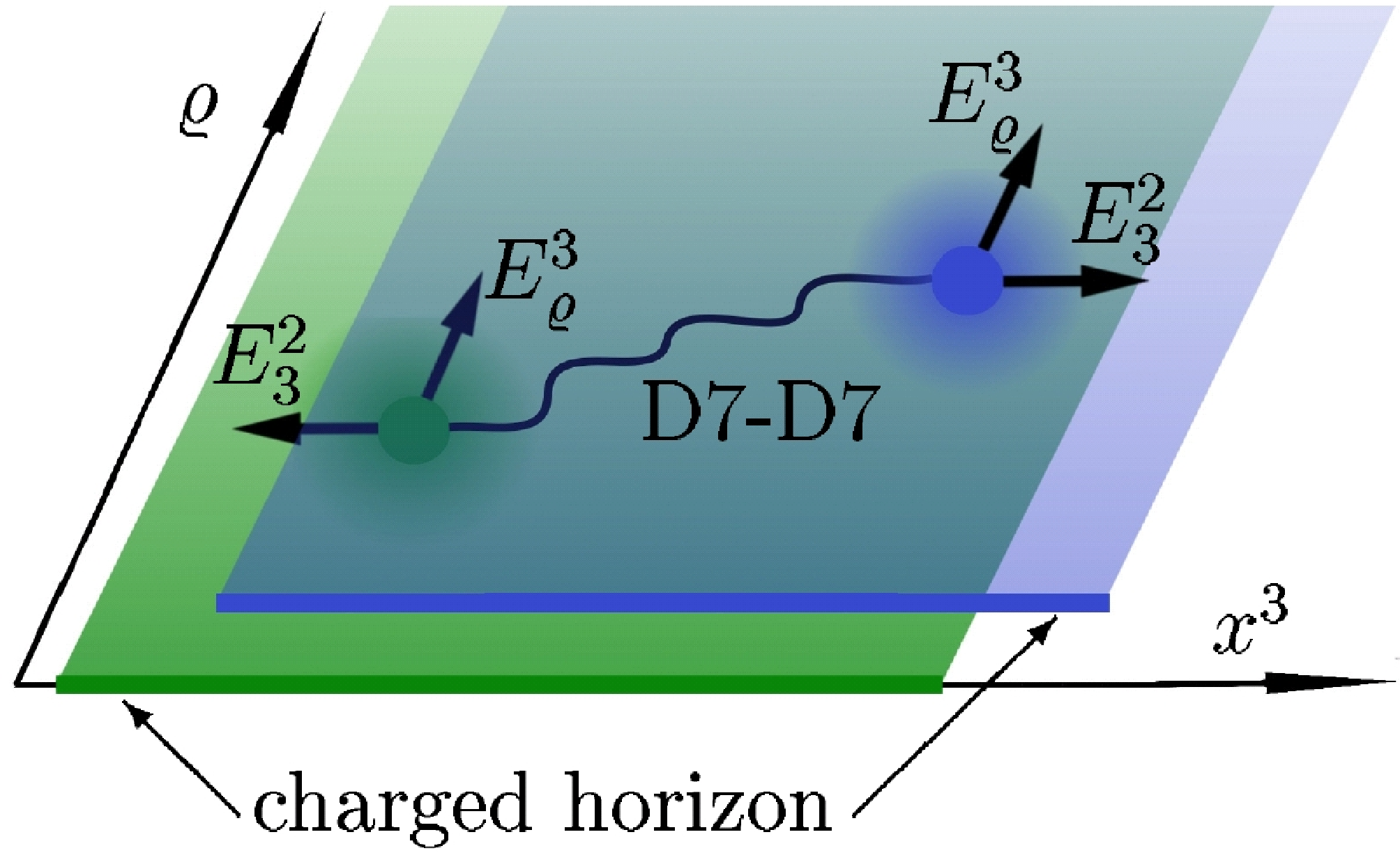
Let us first describe the unstable configuration in absence of the field . As known from [27, 26, 32], the non-zero field is induced by fundamental strings which are stretched from the D-brane to the horizon of the black hole. In the subsequent we call these strings ‘horizon strings’. Since the tension of these strings would increase as they move to the boundary, they are localized at the horizon, i. e. the horizon is effectively charged under the isospin charge given by (1). By increasing the horizon string density, the isospin charge on the D7-brane at the horizon and therefore the energy of the system grows. In [32], the critical density was found beyond which this setup becomes unstable. In this case, the strings would prefer to move towards the boundary due to the repulsive force on their charged endpoints generated by the flavorelectric field .
The setup is now stabilized by the new non-zero field . This field is induced by D-D strings moving in the direction. This movement of the strings may be interpreted as a current in direction which induces the magnetic field . Moreover, the non-Abelian interaction between the D-D strings and the horizon strings induces an flavorelectric field .
From the profile of the gauge fields and their conjugate momenta (see figure 3) we obtain the following: For , i. e. in the normal phase (), the isospin density is exclusively generated at the horizon by the horizon strings. This can also be understood by the profile of the conjugate momenta (see figure 3 (c)). We interpret as the isospin charge located between the horizon at and a fictitious boundary at . In the normal phase, the momentum is constant along the radial direction (see figure 3(c), blue curve), and therefore the isospin density is exclusively generated at the horizon. In the superconducting phase where , i. e. , the momentum is not constant any more. Its value increases monotonically towards the boundary and asymptotes to (see figure 3(c), red curve). Thus the isospin charge is also generated in the bulk and not only at the horizon. This decreases the isospin charge at the horizon and stabilizes the system.
Now we describe the string dynamics which distributes the isospin charge into the bulk. Since the field induced by the D-D strings is non-zero in the superconducting phase, these strings must be responsible for stabilizing this phase. In the normal phase, there are only horizon strings. In the superconducting phase, some of these strings recombine to form D-D strings which correspond to the non-zero gauge field and carry isospin charge 11 1 Note that the D-D strings are of the same order as the horizon strings, namely , since they originate from the DBI action [27].. There are two forces acting on the D-D strings, the flavorelectric force induced by the field and the gravitational force between the strings and the black hole. The flavorelectric force points to the boundary while the gravitational force points to the horizon. The gravitational force is determined by the change in effective string tension, which contains the dependent warp factor. The position of the D-D strings is determined by the equilibrium of these two forces. Therefore the D-D strings propagate from the horizon into the bulk and distribute the isospin charge.
Since the D-D strings induce the field , they also generate the density dual to the condensate , the Cooper pairs. This density is proportional to the D-D strings located in the bulk, in the same way as the density counts the strings which carry isospin charge [26]. This suggest that we can also interpret as the number of D-D strings which are located between the horizon at and the fictitious boundary at . The momentum is always zero at the horizon and increases monotonically in the bulk (see figure 3 (d)). Thus there are no D-D strings at the horizon.
The double importance of the D-D strings is given by the fact that they are both responsible for stabilizing the superconducting phase by lowering the isospin charge density, as well as being the dual of the Cooper pairs since they break the symmetry.


5 Thermodynamics & Phase Transition
In this section we study the thermodynamics of the fundamental matter sector which is dual to the thermal contributions of the D-branes. According the AdS/CFT dictionary the partition function of the boundary field theory is given in terms of the Euclidean on-shell supergravity action ,
| (33) |
Thus the thermodynamical potential, i. e. in the grand canonical ensemble the grand potential , is proportional to the Euclidean on-shell supergravity action,
| (34) |
To calculate the thermal contributions of the D-branes , we have to determine the Euclidean version of the DBI action (14) on-shell.
5.1 Adapted symmetrized trace prescription
Now we calculate the Euclidean on-shell action using the adapted symmetrized trace prescription defined in section 3.2. First we perform a Wick rotation in the time direction. Next we renormalize the action by adding appropriate counterterms (see [49] for a review). Since the action (15) has the same structure as the DBI action in [50, 26, 32] and since in these cases the counterterms do not depend on the finite densities, we can write the counterterms as in [50, 26, 32],
| (35) |
where is the UV-cutoff and
| (36) |
with Minkowski space volume . Then the renormalized Euclidean on-shell action may simply be written as
| (37) |
where determines the minimal value of the coordinate on the D-branes, i. e. for black hole embeddings which we consider exclusively in this paper, and
| (38) |
In figure 4 we plot the dimensionless grand potential defined as
| (39) |
We also calculate the specific heat
| (40) |
where is the free energy in the canonical ensemble 22 2 Note that in [14] we considered the second derivative of the grand potential in the grand canonical ensemble. Although not simply related to the specific heat, that quantity also shows a discontinuity indicating the second order phase transition.. Using (28), the expression for the specific heat can be rewritten as
| (41) |
with . In figure 9 we plot the dimensionless specific heat defined as
| (42) |
Below we discuss that our results hint towards a boson liquid being present. We also comment on the relation of our results to [51].
5.2 Expansion of the DBI action
The thermodynamical behavior in the case of the expanded DBI action may be determined in the same way as for the adapted symmetrized trace prescription. As mentioned above, the counterterms are needed to regularize the action and do not depend on the gauge fields on the brane. They are needed to regularize the divergence which occurs due to the infinite volume of the AdS space. For vanishing gauge fields on the brane, the action calculated using the adapted symmetrized trace prescription and the action expanded in field strength coincide. Thus the counterterms discussed above may also be used to regularize the action expanded in . For the renormalized Euclidean action we obtain
| (43) |
where
| (44) |
with and as defined in equations (29) and (81). In figure 6 we also plot the dimensionless grand potential obtained by the action expanded to fourth order in and defined as
| (45) |
Note that we have not computed the Legendre-transformed action for the DBI action expanded to fourth order due to technical complications discussed in section 3.2.2. Thus we do not have direct access to the quantities in the canonical ensemble, such as the free energy needed to compute the specific heat. A calculation exploiting thermodynamical relations between the ensembles is postponed to future work.
5.3 Thermodynamical consistency
In the following we confirm that both definitions of the grand potential, (39) and (45), give consistent thermodynamics. For this purpose, we have to vary the grand potential with respect to the thermodynamical variables. In the gravity setup this variation is induced by a variation of the gravity fields. Here we only consider a variation of the gauge field , since the variation of the embedding function is the same as in [26]. Using the equations of motion, the variation of the dimensionless grand potential with respect to the gauge field reduces to a boundary term,
| (46) |
Here is given by the integrand of the grand potential. Using the asymptotic behavior of the gauge fields (25), (26), (31) (26), the contribution of the fields and vanishes and the result coincides with [26],
| (47) |
Therefore we confirm that is the thermodynamical potential in the grand canonical ensemble, namely the grand potential. We also see that the density is not a thermodynamical variable.
5.4 Results & Comparison of the two prescriptions
We now compare the results obtained by evaluating the non-Abelian DBI action using the adapted symmetrized trace prescription or the expansion to fourth order.

Figure 4 shows that for non-zero gauge field , a phase transition occurs. The presence of this phase transition does not depend on the prescription used, as seen from the comparison of the potential derived using the adapted symmetrized trace prescription (see figure 5) with the results derived from the expanded DBI action (see figure 6). The transition is second order since there is a discontinuous step in the specific heat , see figure 9.


The temperature scale in the massless case is defined by
| (48) |
where and as obtained from the adapted symmetrized trace prescription (see section 3.2.1). For the expanded DBI action we equivalently obtain and . In the massive case we fix a quark mass , then a chemical potential measured in units of . Thus the temperature scale is defined as
| (49) |
where is the value of the mass parameter at which the phase transition occurs.

From the behavior of the order parameter , see in figure 7, near the critical temperature, we obtain the critical exponent of the transition to be , which coincides with the result obtained from Landau theory. It is also determined numerically from a fit within 10 percent accuracy, see blue dashed curve in figure 7. This exponent is independent from the quark mass as seen from the black curve at shown in figure 7. We have also confirmed numerically that the critical exponent of the order parameter does not depend on the prescription (adapted symmetrized trace or expanded DBI). Since the order parameter and the density increase rapidly as , we expect that the probe approximation breaks down near .

We define the density of superconducting charges in the following way
| (50) |
This identification was suggested in [7]. Beyond the arguments given there, we have the advantage of exactly knowing the dual field theory interpretation and having a string picture, see section 4. The numerator of equation (50) counts the isospin charges present in the bulk excluding those localized at the black hole horizon . Following the ideas described in section 4, these charges may be identified with the D-D strings in the bulk, which are dual to the Cooper pairs. As expected from Ginzburg-Landau theory, this superconducting density vanishes linearly at in massive and massless cases regardless of the prescription chosen, see figure 8.

In figure 9 the dimensionless specific heat computed from the adapted symmetrized trace prescription for massless quarks is shown versus the temperature. It clearly shows a discontinuity at the phase transition, stressing that the observed transition is second order. Note that the dimensionful specific heat is given by , where is the dimensionless specific heat shown in figure 9.
The blue curve in figure 9 corresponds to the normal phase while the red one shows the behavior of the superconducting phase. A general feature of superfluids, including charged superfluids as in the present case, is the behavior of the specific heat near . For Bose liquids the heat capacity has cubic temperature dependence. In Fermi liquids, a linear temperature dependence dominates near . In our numerical results (figure 9) we see a dramatic change of specific heat in the normal phase (blue curve) in sharp contrast to the constant behavior, corresponding to , of the superconducting phase (red curve) close to the critical temperature. The divergent behavior close to is due to the probe approximation which we use. Although our numerics do not allow to extend the calculation up to it is tempting to extrapolate the observed behavior towards and to conclude that our setup in the superconducting phase is a Bose liquid.
Recently a new type of quantum liquid has been discussed in [51], where the authors consider a brane setup at zero mass in the limit of infinite baryon density, i. e. at zero temperature. In that case the heat capacity was found to be proportional to , neither typical for a Fermi nor for a Bose liquid.
In the following we argue that our result found above suggests to consider the possibility of a phase transition also in the baryonic setup [51]. The baryonic setup of [51] may be related to our normal phase by a symmetry between pure baryonic and pure isospin configurations found in [32]. Thus the specific heat in the baryonic setup and in our normal-conducting phase coincide. Since in our isospin case there is a phase transition to the superconducting phase which shows the usual Bose liquid behavior, we suggest the possibility of a similar phase transition in the baryonic setup of [51]. The possible new phase may lead to the usual behavior of a Bose or Fermi liquid.

Summarizing our thermodynamical results in a phase diagram, we obtain figure 10. The choice of the calculational method – adapted symmetrized trace or expansion of the DBI to fourth order – does not change the qualitative structure of the phase diagram. The blue phase indicates the known region of stable mesons surviving the deconfinement transition. It is separated from the white meson melting region by the meson melting transition (blue line), see [52, 25, 50, 26, 29, 27, 53, 32]. Above a critical isospin density marked by the green line, a flavor-superconducting phase forms. At even higher isospin density, our approach, which does not include the back-reaction of the D-brane, gives diverging order parameters, signalling the breakdown of this approach. This particular region is indicated by orange color. Note that this behavior is well-known to occur in systems without back-reaction. In our case, the gauge fields on the D-brane grow arbitrarily large close to zero temperature. This behavior will be cured by including the back-reaction, i. e. the contribution of the gauge fields to the total energy-momentum tensor. For the Abelian Higgs model, it is shown in [13] that similar divergences are removed when these terms are included.
6 Fluctuations
The full gauge field on the branes consists of the field and fluctuations ,
| (51) |
where are the generators. The linearized equations of motion for the fluctuations are obtained by expanding the DBI action in to second order. We will analyze the fluctuations and , .
Including these fluctuations, the DBI action reads
| (52) |
with the non-Abelian field strength tensor
| (53) |
where the background is collected in
| (54) |
and all terms containing fluctuations in the gauge field are summed in
| (55) |
Index anti-symmetrization is always defined with a factor of two in the following way .
6.1 Adapted symmetrized trace prescription
In this section we use the adapted symmetrized trace prescription to determine the fluctuations about the background we discussed in section 3.2.1. To obtain the linearized equations of motion for the fluctuations , we expand the action (52) to second order in fluctuations,
| (56) |
As in the previous paper [33], we collect the metric and gauge field background in the tensor . Using the Euler-Lagrange equation, we get the linearized equation of motion for fluctuations in the form
| (57) |
Note that the linearized version of the fluctuation field strength used in equation (57) is given by
| (58) |
In our specific case the background tensor in its covariant form is given by
| (59) |
Inversion yields the contravariant form needed to compute the explicit equations of motion. The inverse of is defined as 33 3 We calculate the inverse of by ignoring the commutation relation of the ’s because of symmetrized trace. It is important that must not be simplified to since symmetrisation is not the same.. The non-zero components of may be found in the appendix B.1.
Fluctuations in :
For the fluctuation with zero spatial momentum, we obtain the equation of motion
| (60) |
with
| (61) |
Fluctuations in , :
For the fluctuations and with zero spatial momentum, we obtain the coupled equations of motion
| (62) | ||||
| (63) | ||||
where the component of the inverse background tensor may be found in the appendix B.1, index symmetrization is defined and
| (64) |
6.2 Expansion of the DBI action
In this section we determine the equation of motion for the fluctuation in the background determined by the DBI action expanded to fourth order in (see section 3.2.2). To obtain the quadratic action in the field , we first have to expand the DBI action (52) to fourth order in the full gauge field strength , and expand the result to second order in . Due to the symmetries of our setup, the equation of motion for the fluctuation at zero spatial momentum decouples from the other equations of motion, such that we can write down an effective Lagrangian for the fluctuation . This effective Lagrangian is given in the appendix B.2. The equation of motion for with zero spatial momentum determined by the Euler-Lagrange equation is given by
| (65) |
where
| (66) |
We introduce the factors which may be found in the appendix B.2 to emphasize the similarity to the equation of motion obtained by the adapted symmetrized trace prescription (60).
6.3 Result & Comparison of the two prescriptions
6.3.1 Conductivity
We calculate the frequency-dependent conductivity using the Kubo formula,
| (67) |
where is the retarded Green function of the current dual to the fluctuation , which we calculate using the method obtained in [54]. The current is the analog to the electric current since it is charged under the symmetry. In real space it is transverse to the condensate. Since this fluctuation is the only one which transforms as a vector under the rotational symmetry, it decouples from the other fluctuations of the system.
The real part of the frequency-dependent conductivity is presented in figure 11, 12, 13, 15. It shows the appearance and growth of a gap as we increase the condensate . The conductivity gap originates in a pseudo gap already present right above , as can be seen for example from the red curve in figure 11. By pseudo gap we mean a well-defined gap in the conductivity at low frequency in which the conductivity is not identically zero [8]. Both calculational prescriptions – the adapted symmetrized trace prescription and the expansion of the DBI action to fourth order in the field strength – yield qualitatively very similar results as can be seen by comparing figures 13 and 15. As a further distinct effect when using the adapted symmetrized trace prescription, figure 11, 12, 13 show prominent peaks which we interpret as mesonic excitations below. Increasing the quark mass from zero to a finite value, these meson peaks become sharper, i.e. more quasiparticle-like. This is reminiscent of results for condensed matter systems where prominent quasiparticle peaks appear (e. g. [55]). In figure 12 at fixed , the sharp resonances are also present inside the gap. In contrast to the adapted symmetrized trace prescription, from the expanded DBI action we obtain less prominent peaks as seen from figure 15. In the conductivity obtained from the DBI action expanded to fourth order, the peaks do not appear until we approach small temperatures. We expect that the terms higher order in the field strength dominate the generation of the peaks and therefore the generation of the meson mass. If the higher order terms discussed here are included, we presume that the quasinormal modes which generate these peaks move closer to the real axis.


Using the Kramers-Kronig relation, which connects the real and imaginary part of the complex conductivity, we find a delta peak at in the real part of the conductivity, . The corresponding -behavior in the imaginary part is visualized in figure 14. As expected from Ginzburg-Landau theory, our numerics show that the superconducting density vanishes linearly at the critical temperature, for . This field theory definition of the superconducting density yields a quantity with the same linear scaling near as found in our bulk definition (50) of the superconducting density . This confirms that these two quantities may be identified. Our numerics indeed indicate that and are proportional to each other.

Note that for translation invariant systems at finite density, there is a delta peak in the real part of the conductivity even in a normal conducting phase since the charge carriers cannot lose their momentum. This peak is called Drude peak. In our system, however, the charge carriers can dissipate their momentum although our system is translation invariant [56, 57]. The adjoint degrees of freedom can transfer momentum at order while the fundamental degrees of freedom only at order . The adjoint degrees of freedom effectively act as a heat sink into which the flavor fields can dissipate their momentum. Thus we do not observe a Drude peak in our system.

6.3.2 Spectral functions
In order to identify the prominent peaks in the conductivity in terms of field theory quantities as meson resonances, we examine the spectral functions which are related to these conductivities by (67). Due to this relation the prominent peaks in the conductivity correspond to the prominent peaks in the spectral function, see figure 16. As known from [58, 33] the resonances appearing in the spectral functions of vector fields in the bulk correspond to vector meson excitations in the dual field theory. Moving to higher quark mass parameter and near the meson melting transition, we compare the resulting spectrum, see figure 17 to the supersymmetric mass formula obtained in [24]. The prominent peaks clearly approach the supersymmetric line spectrum from above. The same behavior was found in figure 7 of [33], where vector mesons were considered also close to the meson melting transition. Note that the accuracy of our numerics becomes insufficient at larger frequencies around 44 4 The frequency range of validity of our fluctuation numerics increases with quark mass. However, the numerics for the background become worse at large quark masses..


6.3.3 Comments on stability
As shown in figure 18, our setup is stable with respect to the fluctuations and . Furthermore, figure 18 shows that the quasinormal modes of higher excitations move to larger frequencies and closer to the real axis. This corresponds to the formation of stable massive mesons. Such a behavior is known in gauge/gravity duality for mesons which are built from massive quarks (e. g. [33]). Thus we observe a dynamical mass generation for the mesons as described in the following subsection.

6.3.4 Dynamical mass generation
In this section we discuss dynamical mas generation on the field theory and on the gravity side. For this issue, it is important to distinguish between the cases where the broken symmetry is global or local in the boundary field theory.
Field theory observation
As explained in section 3.2, the superconducting condensate breaks the symmetry spontaneously in the field theory living on the AdS boundary. According to the Goldstone theorem this generates one massless Nambu-Goldstone boson in the boundary field theory. Let us now discuss the two different cases:
- Local symmetry:
-
If the broken symmetry is gauged, the Nambu-Goldstone boson is eaten by the gauge field charged under the spontaneously broken symmetry. In conventional superconductors this mechanism gives mass to the photons which implies the Meissner-Ochsenfeld effect.
- Global symmetry:
-
If the broken symmetry is global, there is no dynamical gauge field which eats the Nambu-Goldstone boson. Thus the Nambu-Goldstone boson remains present in the spectrum. Since this is the case in our setup, we need to identify this Nambu-Goldstone boson in the spectrum. In general, the Nambu-Goldstone boson corresponds to the phase of the condensate which parametrizes the the coset space . In our setup, the fluctuations and defined above (62) are charged under the symmetry such that the Nambu-Goldstone boson can be found in these fluctuations (see fig. 18).
Although in our case the broken symmetry is global, we nevertheless observe dynamical mass generation as see for instance in figures 16 and 18. Therefore in our setup, a more subtle mechanism then the ordinary Higgs mechanism generates the meson masses dynamically. Let us explain this mechanism in the dual gravity setup.
Gravity explanation
According to the AdS/CFT dictionary, a global symmetry in the boundary field theory is mapped to a local symmetry in the gravity theory. Thus the symmetry of the two D-branes is local in the gravity theory. In this paper we find new solutions to the equations of motion which non-vanishing gauge field components and . Since the gravity action is unchanged and thus still invariant, this non-zero components break the gauge symmetry spontaneously which generates in total three Nambu-Goldstone bosons. They are eaten by the gauge fields which then become massive. Let us now discuss the corresponding mass terms in more detail.
First we consider a non-zero isospin chemical potential which generates the mass term for the fluctuations . This new term shifts the quadratic fluctuation term in the action, i.e. its energy by the value of the field . For the spectral function of the dual field theory this results in a shift of the meson resonance peaks, see [33].
Second we consider the non-zero gauge field component which generates a mass term for the fluctuation . We expect that this mass term shifts the quasinormal frequencies of this system in the complex plane. That results in generation and shift of the resonance peaks in the spectral function as well as generation of the gap structure in the conductivity. To make more precise statements, the spectrum of quasinormal modes needs to be studied in presence of these fields.
7 Meissner-Ochsenfeld effect
The Meissner effect is a distinct signature of conventional and unconventional superconductors. It is the phenomenon of expulsion of external magnetic fields. An induced current in the superconductor generates a magnetic field counter-acting the external magnetic field . In AdS/CFT we are not able to observe the generation of counter-fields since the symmetries on the boundary are always global. Nevertheless, we can study their cause, i.e. the current induced in the superconductor. As usual [4, 5, 9, 13, 6, 18] the philosophy here is to weakly gauge the boundary theory afterwards.
In order to investigate how an external magnetic field influences our p-wave superconductor, we have two choices. Either we introduce the field along the spatial -direction or equivalently one along the -direction i.e. . Both are “aligned” with the spontaneously broken -flavor direction.
As an example here we choose a non-vanishing . This requires inclusion of some more non-vanishing field strength components in addition to those given in equation (11). In particular we choose and yielding the additional components55 5 Close to the phase transition, it is consistent to drop the dependence of the field on . Away form the phase transition the dependence must be included. From the boundary asymptotics it will be possible to extract the magnetic field and the magnetization of the superconductor.
| (68) |
Recall that the radial AdS-direction is identified by the indices either or . Amending the DBI-action (14) with the additional components (68), we compute the determinant in analogy to equation (14). We then choose to expand the new action to second order in , i.e. we only consider terms being at most quadratic in the fields. This procedure gives the truncated DBI action
| (69) |
Respecting the symmetries and variable dependencies in our specific system, this can be written as
| (70) |
with the convenient redefinitions
| (71) |
Rescaling the -coordinate once more
| (72) |
the equations of motion derived from the action (70) take a simple form
| (73) |
Here all metric components are understood to be evaluated at and .
We aim at decoupling and solving the system of partial differential equations (73) by the product ansatz
| (74) |
For this ansatz to work, we need to make two assumptions: First we assume that is constant in . Second we assume that is small, which clearly is the case near the transition . Our second assumption prevents from receiving a dependence on through its coupling to . These assumptions allow to write the second equation in (73) as
| (75) |
All terms but the last one are independent of , so the product ansatz (74) is consistent only if
| (76) |
where is a constant. The differential equation (76) has a particular solution if . The solutions for are Hermite functions
| (77) |
which have Gaussian decay at large . Choosing the lowest solution with and , which has no nodes, is most likely to give the configuration with lowest energy content. So the system we need to solve is finally given by
| (78) |
Asymptotically near the horizon the fields take the form
| (79) | ||||||||||
while at the boundary we obtain
| (80) | ||||||||||
We succeed in finding numerical solutions and to the set of equations (78) obeying the asymptotics given by equations (79) and (80). These numerical solutions are used to approach the phase transition from the superconducting phase by increasing the magnetic field. We map out the line of critical temperature-magnetic field pairs in figure 19. In this way we obtain a phase diagram displaying the Meissner effect. The critical line in figure 19 separates the phase with and without superconducting condensate .
We emphasize that this is a background calculation involving no fluctuations. Complementary to the procedure described above we also confirmed the phase diagram using the instability of the normal phase against fluctuations. Starting at large magnetic field and vanishing condensate , we determine for a given magnetic field the temperature at which the fluctuation becomes unstable. That instability signals the condensation process into the superconducting phase.

The presence of the coexistence phase below the critical line, where the system is still superconducting despite the presence of an external magnetic field, is the signal of the Meissner effect in the case of a global symmetry considered here. If we now weakly gauged the flavor symmetry at the boundary, the superconducting current would generate a magnetic field opposite to the external field. Thus the phase observed is a necessary condition in the case of a global symmetry for finding the standard Meissner effect when gauging the symmetry.
8 Discussion and Outlook
We found a holographic realization of superconductivity in the context of gauge/gravity duality with flavor at finite isospin chemical potential, for which the field theory action is known explicitly. The condensation process corresponds to a recombination of strings which leads to a thermodynamically favored configuration. On the field theory side, this new state may be interpreted as a meson superfluid. We show that the superconducting phase persists at finite quark mass and find a holographic Meissner–Ochsenfeld effect. From a technical point of view, we compare two different approaches for evaluating the non-Abelian DBI action involved (expansion to fourth order and a new modified trace evaluation procedure which we propose) and find the same physical results in both approaches, at least qualitatively.
For the future, we expect that a holographic s-wave superconductor may be constructed by applying the methods presented to the transverse scalars in similar holographic setups. It will also be interesting to apply our methods to the configuration discussed in [48] in order to find a purely fermionic superconductor.
Acknowledgements
We are grateful to T. Dahm, S. Gubser, S. Hartnoll, C. Herzog, K. Landsteiner, R. Meyer, A. O’Bannon, S. Pufu, F. Rust and E. Tsatis for discussions. This work was supported in part by The Cluster of Excellence for Fundamental Physics - Origin and Structure of the Universe.
Appendix A Expansion of the DBI action to fourth order
In this section we give some lengthy equations needed to calculate the expanded DBI action and the resulting equations of motion (see section 3.2.2).
The which determine the terms in expanded DBI action at order in the field strength are given by
| (81) |
with
| (82) |
Using the Euler-Lagrange equation the resulting equations of motion are
| (83) |
with
| (84) |
Appendix B Fluctuations
B.1 Adapted symmetrized trace prescription
In this section we present the elements of the inverse background tensor defined in section 6.1. The diagonal elements are given by
| (85) |
where the other diagonal elements are just . The off-diagonal elements read
| (86) | ||||
The denominator is given by
| (87) |
B.2 Expansion of the DBI action to fourth order
In this section we calculate the quadratic action for the fluctuations using the expanded DBI action as explained in section 6.2. Since the fluctuation decouples from every other fluctuation we can write down an effective Lagrangian for this fluctuation. This Lagrangian is given by
| (88) |
Using the results for the symmetrized traces (30), the effective Lagrangian simplifies to
| (89) |
To simplify the equation of motion for the fluctuation (see (65)) we define
| (90) |
References
- [1] J. M. Maldacena, The large N limit of superconformal field theories and supergravity, Adv. Theor. Math. Phys. 2 (1998) 231–252, arXiv:hep-th/9711200.
- [2] E. Witten, Anti-de Sitter space, thermal phase transition, and confinement in gauge theories, Adv. Theor. Math. Phys. 2 (1998) 505–532, arXiv:hep-th/9803131.
- [3] S. A. Hartnoll, C. P. Herzog, and G. T. Horowitz, Building a Holographic Superconductor, Phys. Rev. Lett. 101 (2008) 031601, arXiv:0803.3295.
- [4] E. Nakano and W.-Y. Wen, Critical magnetic field in a holographic superconductor, Phys. Rev. D78 (2008) 046004, arXiv:0804.3180.
- [5] T. Albash and C. V. Johnson, A Holographic Superconductor in an External Magnetic Field, JHEP 09 (2008) 121, arXiv:0804.3466.
- [6] W.-Y. Wen, Inhomogeneous magnetic field in AdS/CFT superconductor, arXiv:0805.1550.
- [7] S. S. Gubser and S. S. Pufu, The gravity dual of a p-wave superconductor, JHEP 11 (2008) 033, arXiv:0805.2960.
- [8] M. M. Roberts and S. A. Hartnoll, Pseudogap and time reversal breaking in a holographic superconductor, JHEP 08 (2008) 035, arXiv:0805.3898.
- [9] K. Maeda and T. Okamura, Characteristic length of an AdS/CFT superconductor, Phys. Rev. D78 (2008) 106006, arXiv:0809.3079.
- [10] C. P. Herzog, P. K. Kovtun, and D. T. Son, Holographic model of superfluidity, arXiv:0809.4870.
- [11] P. Basu, A. Mukherjee, and H.-H. Shieh, Supercurrent: Vector Hair for an AdS Black Hole, Phys. Rev. D79 (2009) 045010, arXiv:0809.4494.
- [12] G. T. Horowitz and M. M. Roberts, Holographic Superconductors with Various Condensates, Phys. Rev. D78 (2008) 126008, arXiv:0810.1077.
- [13] S. A. Hartnoll, C. P. Herzog, and G. T. Horowitz, Holographic Superconductors, JHEP 12 (2008) 015, arXiv:0810.1563.
- [14] M. Ammon, J. Erdmenger, M. Kaminski, and P. Kerner, Superconductivity from gauge/gravity duality with flavor, accepted for publication in Physics Letters B arXiv:0810.2316.
- [15] P. Basu, J. He, A. Mukherjee, and H.-H. Shieh, Superconductivity from D3/D7: Holographic Pion Superfluid, arXiv:0810.3970.
- [16] S. S. Gubser and A. Nellore, Low-temperature behavior of the Abelian Higgs model in anti-de Sitter space, JHEP 04 (2009) 008, arXiv:0810.4554.
- [17] A. O’Bannon, Toward a Holographic Model of Superconducting Fermions, JHEP 01 (2009) 074, arXiv:0811.0198.
- [18] A. Rebhan, A. Schmitt, and S. A. Stricker, Meson supercurrents and the Meissner effect in the Sakai- Sugimoto model, JHEP 05 (2009) 084, arXiv:0811.3533.
- [19] N. Evans and E. Threlfall, Chemical Potential in the Gravity Dual of a 2+1 Dimensional System, Phys. Rev. D79 (2009) 066008, arXiv:0812.3273.
- [20] F. Denef and S. A. Hartnoll, Landscape of superconducting membranes, Phys. Rev. D79 (2009) 126008, arXiv:0901.1160.
- [21] G. Koutsoumbas, E. Papantonopoulos, and G. Siopsis, Exact Gravity Dual of a Gapless Superconductor, JHEP 07 (2009) 026, arXiv:0902.0733.
- [22] C. P. Herzog and S. S. Pufu, The Second Sound of SU(2), JHEP 04 (2009) 126, arXiv:0902.0409.
- [23] A. Karch and E. Katz, Adding flavor to AdS/CFT, JHEP 06 (2002) 043, arXiv:hep-th/0205236.
- [24] M. Kruczenski, D. Mateos, R. C. Myers, and D. J. Winters, Meson spectroscopy in AdS/CFT with flavour, JHEP 07 (2003) 049, arXiv:hep-th/0304032.
- [25] J. Babington, J. Erdmenger, N. J. Evans, Z. Guralnik, and I. Kirsch, Chiral symmetry breaking and pions in non-supersymmetric gauge / gravity duals, Phys. Rev. D69 (2004) 066007, arXiv:hep-th/0306018.
- [26] S. Kobayashi, D. Mateos, S. Matsuura, R. C. Myers, and R. M. Thomson, Holographic phase transitions at finite baryon density, JHEP 02 (2007) 016, arXiv:hep-th/0611099.
- [27] A. Karch and A. O’Bannon, Holographic Thermodynamics at Finite Baryon Density: Some Exact Results, JHEP 11 (2007) 074, arXiv:0709.0570.
- [28] K. Ghoroku, M. Ishihara, and A. Nakamura, D3/D7 holographic Gauge theory and Chemical potential, Phys. Rev. D76 (2007) 124006, arXiv:0708.3706.
- [29] D. Mateos, S. Matsuura, R. C. Myers, and R. M. Thomson, Holographic phase transitions at finite chemical potential, JHEP 11 (2007) 085, arXiv:0709.1225.
- [30] S. Nakamura, Y. Seo, S.-J. Sin, and K. P. Yogendran, A new phase at finite quark density from AdS/CFT, J. Korean Phys. Soc. 52 (2008) 1734–1739, arXiv:hep-th/0611021.
- [31] S. Nakamura, Y. Seo, S.-J. Sin, and K. P. Yogendran, Baryon-charge Chemical Potential in AdS/CFT, Prog. Theor. Phys. 120 (2008) 51–76, arXiv:0708.2818.
- [32] J. Erdmenger, M. Kaminski, P. Kerner, and F. Rust, Finite baryon and isospin chemical potential in AdS/CFT with flavor, JHEP 11 (2008) 031, arXiv:0807.2663.
- [33] J. Erdmenger, M. Kaminski, and F. Rust, Holographic vector mesons from spectral functions at finite baryon or isospin density, Phys. Rev. D77 (2008) 046005, arXiv:0710.0334.
- [34] R. Apreda, J. Erdmenger, N. Evans, and Z. Guralnik, Strong coupling effective Higgs potential and a first order thermal phase transition from AdS/CFT duality, Phys. Rev. D71 (2005) 126002, arXiv:hep-th/0504151.
- [35] A. Buchel, J. Jia, and V. A. Miransky, Dynamical stabilization of runaway potentials at finite density, Phys. Lett. B647 (2007) 305–308, arXiv:hep-th/0609031.
- [36] O. Aharony, K. Peeters, J. Sonnenschein, and M. Zamaklar, Rho meson condensation at finite isospin chemical potential in a holographic model for QCD, JHEP 02 (2008) 071, arXiv:0709.3948.
- [37] G. E. Brown and M. Rho, Scaling effective Lagrangians in a dense medium, Phys. Rev. Lett. 66 (1991) 2720–2723.
- [38] F. Sannino, General structure of relativistic vector condensation, Phys. Rev. D67 (2003) 054006, arXiv:hep-ph/0211367.
- [39] D. Mateos and L. Patino, Bright branes for strongly coupled plasmas, JHEP 11 (2007) 025, arXiv:0709.2168.
- [40] D. T. Son and M. A. Stephanov, QCD at finite isospin density, Phys. Rev. Lett. 86 (2001) 592–595, arXiv:hep-ph/0005225.
- [41] D. T. Son and M. A. Stephanov, QCD at finite isospin density: From pion to quark antiquark condensation, Phys. Atom. Nucl. 64 (2001) 834–842, arXiv:hep-ph/0011365.
- [42] J. B. Kogut and D. K. Sinclair, Lattice QCD at finite isospin density at zero and finite temperature, Phys. Rev. D66 (2002) 034505, arXiv:hep-lat/0202028.
- [43] J. Erdmenger, N. Evans, I. Kirsch, and E. Threlfall, Mesons in Gauge/Gravity Duals - A Review, Eur. Phys. J. A35 (2008) 81–133, arXiv:0711.4467.
- [44] R. C. Myers, Dielectric-branes, JHEP 12 (1999) 022, arXiv:hep-th/9910053.
- [45] A. A. Tseytlin, On non-abelian generalisation of the Born-Infeld action in string theory, Nucl. Phys. B501 (1997) 41–52, arXiv:hep-th/9701125.
- [46] A. Hashimoto and W. Taylor, Fluctuation spectra of tilted and intersecting D-branes from the Born-Infeld action, Nucl. Phys. B503 (1997) 193–219, arXiv:hep-th/9703217.
- [47] N. R. Constable, R. C. Myers, and O. Tafjord, The noncommutative bion core, Phys. Rev. D61 (2000) 106009, arXiv:hep-th/9911136.
- [48] R. C. Myers and M. C. Wapler, Transport Properties of Holographic Defects, JHEP 12 (2008) 115, arXiv:0811.0480.
- [49] A. Karch, A. O’Bannon, and K. Skenderis, Holographic renormalization of probe D-branes in AdS/CFT, JHEP 04 (2006) 015, arXiv:hep-th/0512125.
- [50] D. Mateos, R. C. Myers, and R. M. Thomson, Thermodynamics of the brane, JHEP 05 (2007) 067, arXiv:hep-th/0701132.
- [51] A. Karch, D. T. Son, and A. O. Starinets, Zero Sound from Holography, arXiv:0806.3796.
- [52] T. Faulkner and H. Liu, Condensed matter physics of a strongly coupled gauge theory with quarks: some novel features of the phase diagram, arXiv:0812.4278.
- [53] C. Hoyos-Badajoz, K. Landsteiner, and S. Montero, Holographic Meson Melting, JHEP 04 (2007) 031, arXiv:hep-th/0612169.
- [54] D. T. Son and A. O. Starinets, Minkowski-space correlators in AdS/CFT correspondence: Recipe and applications, JHEP 09 (2002) 042, arXiv:hep-th/0205051.
- [55] M. Tinkham, The electromagnetic properties of superconductors, Rev. Mod. Phys. 46 (Oct, 1974) 587–596.
- [56] A. Karch and A. O’Bannon, Metallic AdS/CFT, JHEP 09 (2007) 024, arXiv:0705.3870.
- [57] A. Karch, A. O’Bannon, and E. Thompson, The Stress-Energy Tensor of Flavor Fields from AdS/CFT, JHEP 04 (2009) 021, arXiv:0812.3629.
- [58] R. C. Myers, A. O. Starinets, and R. M. Thomson, Holographic spectral functions and diffusion constants for fundamental matter, JHEP 11 (2007) 091, arXiv:0706.0162.