Thin film dynamics with surfactant phase transition

The stability and dynamics of thin liquid films have been of considerable interest to both experimental and theoretical research [1, 2, 3, 4]. When the thickness of a flat liquid film is in the range of $\sim 100\,\mathrm{nm}$, it becomes sensitive to interaction with its substrate. In a certain range of film thickness determined by the exact form of the interaction potential, this will render the film unstable with respect to small perturbations and a pattern formation process sets in. Depending on its initial height, the film breaks up into droplets, labyrinth-like patterns or arrays of holes [5, 4]. This process is known as spinodal dewetting.

Brought onto the surface of a liquid film, an insoluble surfactant, for example an organic molecule with a hydrophilic head group and a hydrophobic tail group, alters the surface tension and thereby influences the breakup process. In addition, gradients of surfactant density lead to so-called Marangoni convection on the surface resulting in new instabilities like surfactant-induced fingering [6, 7].

Most surfactants exhibit complicated thermodynamics with several phase transitions [8, 9]. These affect thin film hydrodynamics via an equation of state, relating surface tension to surfactant density [10]. In studies of the dynamics of surfactant covered thin films, surfactant thermodynamics has so far not been paid much attention to, because the hydrodynamics is dominated by Marangoni convection rather than by effects of lateral pressure and diffusion [11].

However, there is a special focus of experimental research on pattern formation under conditions close to the so-called main transition in monolayers of lipids like pulmonary surfactant Dipalmitoylphosphatidylcholine (DPPC) [12, 13, 14]. In vicinity of this first-order phase transition parts of the surfactant in the liquid-expanded (LE) phase and in the liquid-condensed (LC) phase coexist. In these experiments, a substrate is coated with a lipid monolayer via Langmuir-Blodgett transfer, i.e. it is withdrawn from a trough filled with water on which a lipid monolayer has been prepared. The observed patterns consist of ordered arrays of LE and LC domains, including regular stripes and rectangles, the formation of which is usually attributed to oscillations of the meniscus between the water in the trough and the substrate [14]. A full understanding of these phenomena cannot be achieved without understanding the dynamics of the film and the surfactant near the main transition. The aim of this letter is to outline theoretical description of the evolution of a thin film covered with a surfactant undergoing a phase transition.

The model we are going to present is derived within the lubrication approximation [1]. We follow the usual approach [15, 7, 16, 17, 18] to describe the time evolution of the surfactant covered thin film by two coupled partial differential equations, describing the height profile of the underlying liquid film and the surfactant density. The surfactant phase transition is incorporated by choice of a suitable free-energy functional which determines the lateral pressure as well as the diffusive flux. We are going to perform a linear stability analysis of stationary homogeneous solutions of the derived equations and investigate the effect of the surfactant on drop formation by numerical simulations.

We consider a thin liquid film covered with an insoluble surfactant on a moving solid substrate (see fig. 1). The velocity field of the liquid film can be obtained within the lubrication approximation [1]. By this procedure the initially three-dimensional flow problem is reduced to an effectively two-dimensional one. The liquid film is then described by a height profile $h(x,y,t)$, which indicates the local film thickness, and the two-dimensional flow field at the surface ${\bf\tilde{u}}(x,y,t)$. The surfactant density at the surface above the point $(x,y)$ is described by the function $\gamma(x,y,t)$. The continuity equation of an insoluble surfactant has been the subject of considerable discussion [19, 20, 21]. Surface geometry is of negligible influence in the lubrication regime, leaving us with the nondimensionalized conservation law

$$\Gamma_{,T}=-\nabla\cdot\left[\Gamma{\bf\tilde{U}}+{\bf I}\right]\,,$$

(1)

where ${\bf I}$ is the diffusive flux of the surfactant. Here we have scaled all quantities by characteristic values:

		$\displaystyle X=\frac{\epsilon x}{h_{0}}\,,\qquad Y=\frac{\epsilon y}{h_{0}}\,,\qquad T=\frac{\epsilon u_{0}t}{h_{0}}\,,$
		$\displaystyle{\bf U}=\frac{{\bf u}}{u_{0}}\,,\qquad\Gamma=\frac{\gamma}{\gamma_{0}}\,,\qquad{\bf I}=\frac{{\bf i}}{\gamma_{0}u_{0}}\,,$		(2)

and $\nabla:=(\partial_{X},\partial_{Y})$ denotes the nabla operator in non-dimensional coordinates $X,Y$. The dimensionless parameter $\epsilon=h_{0}/l_{0}$ defines the ratio of characteristic height and length scales of the problem. Neglecting surface forces, the flow field at the surface ${\bf\tilde{U}}$, subject to a no-slip condition at the moving substrate, is given by

$${\bf\tilde{U}}=-\frac{H^{2}}{2}\nabla\bar{P}+H\epsilon\mathrm{Ca}^{-1}\nabla\frac{\sigma}{\sigma_{0}}-\frac{{\bf v_{0}}}{u_{0}}\,.$$

(3)

Here $H=h/h_{0}$ denotes the nondimensionalized film height, ${\bf v_{0}}$ stands for the substrate velocity, $\sigma_{0}$ describes the surface tension in absence of any surfactant, and $\mathrm{Ca}=\mu u_{0}/\sigma_{0}$ is the capillary number with dynamic viscosity $\mu$. Moreover, $\bar{P}$ is a generalized pressure given by

$$\bar{P}=-\epsilon^{3}\mathrm{Ca}^{-1}\frac{\sigma}{\sigma_{0}}\nabla^{2}H+\Pi(H)\,.$$

(4)

One can see that $\bar{P}$ contains, besides the Laplace pressure term $\sim\nabla^{2}H$, the disjoining pressure $\Pi(H)$ due to interaction of substrate and liquid. In the literature, different expressions for the disjoining pressure have been considered (see ref. [1] and references therein for a discussion of possible $\Pi(H)$). Here, we will use the expression

$$\Pi(H)=\frac{A_{n}}{H^{n}}-\frac{A_{m}}{H^{m}}\,,$$

(5)

with the positive Hamaker constants $A_{n,m}$, where $m>n$, for example $n=3,m=9$ for Lennard-Jones potentials. The repulsive short-range interaction prevents a complete dry-off and the substrate is always covered with a thin precursor film. Gravity could be accounted for by adding a term $GH$ to $\bar{P}$, but is not considered here since it plays a minor role in the capillary regime.

For the height profile of the liquid film, we obtain the standard evolution equation [1]

$$H_{,T}=-\nabla\cdot\left[-\frac{H^{3}}{3}\nabla\bar{P}+\frac{H^{2}}{2}\epsilon\mathrm{Ca}^{-1}\nabla\frac{\sigma}{\sigma_{0}}-H\frac{{\bf v_{0}}}{u_{0}}\right]\,.$$

(6)

It should be noted, that surfactant thermodynamics affects the system in two ways. First of all, the diffusive flux ${\bf I}$ is determined by the chemical potential of the surfactant. Second, the presence of a surfactant alters the surface tension $\sigma$ of the liquid film, making it dependent on $\gamma$ in a way determined by ehe equation of state of the surfactant. These two points are discussed in further details in the following section.

The lateral pressure $p_{\mathrm{lat}}$ of a surfactant is defined by [22]

$$\sigma(\gamma)=\sigma_{0}-p_{\mathrm{lat}}(\gamma)\,.$$

(7)

Experimentally, $p_{\mathrm{lat}}(\gamma)$ is usually obtained from surface tensions measurements using a film balance, where the available area per surfactant molecule is adjusted with the help of a movable barrier [8, 9, 22]. The resulting isotherms of material exhibiting the first-order LE/LC transition display a behaviour reminiscent of a three-dimensional van der Waals gas. It is therefore reasonable to model the surfactant thermodynamics close to the main transition by a free energy suitable for a two-dimensional analogue of a van der Waals gas. Since the surfactant density varies along the surface, we apply a Cahn-Hilliard-type free-energy functional [23], allowing for a non-uniform free-energy density:

$$\mathcal{F}[\gamma]=\int\mathrm{d}^{D-1}x\left\{\frac{\kappa}{2}\left(\nabla\gamma\right)^{2}+f_{\mathrm{hom}}(\gamma)\right\}\,,$$

(8)

where $\kappa>0$ is constant and $f_{\mathrm{hom}}(\gamma)$ denotes the free-energy density of a homogeneous system with surfactant density $\gamma$. Assuming the system to be in local thermodynamic equilibrium the corresponding lateral pressure is given by [24]

$$p_{\mathrm{lat}}(\gamma)=-f(\gamma)+\gamma\mu^{\mathrm{(chem)}}(\gamma)\,,$$

(9)

where the chemical potential $\mu^{\mathrm{(chem)}}$ is obtained from $\mathcal{F}$ by functional derivation:

$$\mu^{\mathrm{(chem)}}=\frac{\delta\mathcal{F}}{\delta\gamma}=-\kappa\nabla^{2}\gamma+\frac{\partial f_{\mathrm{hom}}}{\partial\gamma}\,.$$

(10)

So far, there have been no limitations on the choice of $f_{\mathrm{hom}}$. In the spirit of Landau’s theory of first-order phase transitions [25] we will now restrict ourselves to free-energy densities that can be approximated sufficiently well by a fourth-order polynomial around the critical density $\gamma_{cr}$ of the main transition. Defining $\tilde{\gamma}=\gamma-\gamma_{\mathrm{cr}}$ we obtain

$$f_{\mathrm{hom}}(\tilde{\gamma})=f_{0}+f_{1}\tilde{\gamma}+f_{2}\tilde{\gamma}^{2}+f_{3}\tilde{\gamma}^{3}+f_{4}\tilde{\gamma}^{4}\,.$$

(11)

Realistic values for the parameters $f_{i}$ can be estimated by fitting eq. (9) to experimentally obtained isotherms. Notice, that $p_{\mathrm{lat}}$ has to be matched to the measured pressure within the coexistence region with the help of a Maxwell construction.

The diffusive current ${\bf I}$ in eq. (1) is proportional to the gradient of $\mu^{\mathrm{(chem)}}$ with proportionality constant $\alpha$ [26]. Hence, in nondimensionalized form, the lateral pressure and the diffusive current can be written as

	$\displaystyle P_{\mathrm{lat}}=$	$\displaystyle-\epsilon^{2}K\left[\frac{1}{2}\left(\nabla\Gamma\right)^{2}+\left(\Gamma_{\mathrm{cr}}+\tilde{\Gamma}\right)\nabla^{2}\Gamma\right]$
		$\displaystyle-F_{\mathrm{hom}}+\left(\Gamma_{\mathrm{cr}}+\tilde{\Gamma}\right)\frac{\partial F_{\mathrm{hom}}}{\partial\tilde{\Gamma}}\,,$		(12)

	$\displaystyle{\bf I}=$	$\displaystyle-\epsilon A\frac{\gamma_{0}}{\sigma_{0}}\nabla\mu^{\mathrm{(chem)}}$
	$\displaystyle=$	$\displaystyle-\epsilon A\left[-\epsilon^{2}K\nabla^{3}\Gamma+\frac{\partial^{2}F_{\mathrm{hom}}}{\partial\tilde{\Gamma}^{2}}\nabla\Gamma\right]\,.$		(13)

Here, the dimensionless numbers $A$ and $K$ are defined by

$$A=\frac{\alpha\sigma_{0}}{h_{0}\gamma_{0}^{2}u_{0}}\,,\qquad K=\frac{\kappa\gamma_{0}^{2}}{h_{0}^{2}\sigma_{0}}\,,$$

(14)

and the nondimensionalized free-energy density of the homogeneous system is given by

$$F_{\mathrm{hom}}=\sum_{n=0}^{4}F_{n}\tilde{\Gamma}^{n}\,,\quad\textrm{ where }\quad F_{n}=\frac{f_{n}}{\sigma_{0}}\gamma_{0}^{n}\,.$$

(15)

Inserting eqs. (12) and (13) into the evolution equations (1) and (6), we obtain the complete set of governing equations:

	$\displaystyle H_{,T}=$	$\displaystyle-\nabla\cdot\left[\frac{H^{3}}{3}\nabla\left\{\epsilon^{3}\mathrm{Ca}^{-1}\left(1-P_{\mathrm{lat}}(\Gamma)\right)\nabla^{2}H-\Pi(H)\right\}\right.$
		$\displaystyle\left.-\epsilon\frac{H^{2}}{2}\mathrm{Ca}^{-1}\nabla P_{\mathrm{lat}}(\Gamma)-H\frac{{\bf v_{0}}}{u_{0}}\right]\,,$		(16)
	$\displaystyle\Gamma_{,T}=$	$\displaystyle-\nabla\cdot\left(\Gamma\left[\frac{H^{2}}{2}\nabla\left\{\epsilon^{3}\mathrm{Ca}^{-1}\left(1-P_{\mathrm{lat}}(\Gamma)\right)\nabla^{2}H\right.\right.\right.$
		$\displaystyle\left.\left.-\Pi(H)\right\}-\epsilon H\mathrm{Ca}^{-1}\nabla P_{\mathrm{lat}}(\Gamma)-\frac{{\bf v_{0}}}{u_{0}}\right]$
		$\displaystyle\left.+\epsilon A\left[\epsilon^{2}K\nabla^{3}\Gamma-\frac{\partial^{2}F_{\mathrm{hom}}}{\partial\tilde{\Gamma}^{2}}\nabla\Gamma\right]\right)\,.$		(17)

In the next section, we will investigate the linear stability of stationary homogeneous solutions of these equations.

In the following we concentrate on the case of a substrate at rest, ${\bf v_{0}}=0$. For the sake of simplicity, we first consider only one-dimensional fields $H(X,T),\,\Gamma(X,T)$. Homogeneous film heights and surfactant densities $H=\hat{H}=\mathrm{const.},\Gamma=\hat{\Gamma}=\mathrm{const.}$ are always stationary solutions of the equations. Expanding eqs. (16) and (17) like $H(X,T)=\hat{H}+\eta(X,T)$ and $\Gamma(X,T)=\hat{\Gamma}+\zeta(X,T)$ yields the linearised set of equations

$$\partial_{T}\left(\begin{array}[]{c}\eta\\ \zeta\end{array}\right)=\mathcal{A}\left(\begin{array}[]{c}\eta\\ \zeta\end{array}\right)\,,$$

(18)

with the linear operator

$$\mathcal{A}=\left(\begin{array}[]{cc}\displaystyle\frac{\hat{H}^{3}}{3}\left(\frac{\partial\Pi}{\partial H}\bigg|_{\hat{H}}\partial_{X}^{2}-\epsilon^{3}\mathrm{Ca}^{-1}\hat{\Sigma}\partial_{X}^{4}\right)&\displaystyle\epsilon\mathrm{Ca}^{-1}\frac{\hat{H}^{2}}{2}\hat{\Gamma}\left(\frac{\partial^{2}F_{\mathrm{hom}}}{\partial\tilde{\Gamma}^{2}}\bigg|_{\Delta\Gamma}\partial_{X}^{2}-\epsilon^{2}K\partial_{X}^{4}\right)\\ \displaystyle\hat{\Gamma}\frac{\hat{H}^{2}}{2}\left(\frac{\partial\Pi}{\partial H}\bigg|_{\hat{H}}\partial_{X}^{2}-\epsilon^{3}\mathrm{Ca}^{-1}\hat{\Sigma}\partial_{X}^{4}\right)&\displaystyle\epsilon\left(\hat{\Gamma}^{2}\hat{H}\mathrm{Ca}^{-1}+A\right)\left(\frac{\partial^{2}F_{\mathrm{hom}}}{\partial\tilde{\Gamma}^{2}}\bigg|_{\Delta\Gamma}\partial_{X}^{2}-\epsilon^{2}K\partial_{X}^{4}\right)\end{array}\right)$$

(19)

where $\hat{\Sigma}=\sigma(\gamma_{0}\hat{\Gamma})/\sigma_{0}$ and $\Delta\Gamma=\hat{\Gamma}-\Gamma_{\mathrm{cr}}$. Using the ansatz $\eta\sim\exp(\lambda T+\mathrm{i}kX)$, $\zeta\sim\exp(\lambda T+\mathrm{i}kX)$, trace $\tau$ and determinant $\Delta$ of the resulting matrix ${\bf\mathrm{A}}={\bf\mathrm{A}}(k)$ can be obtained as polynomials of wavenumber $k$. The growth rates $\lambda$, which are the eigenvalues of ${\bf\mathrm{A}}(k)$, can be calculated by use of

$$\lambda_{\pm}=\frac{\tau\pm\sqrt{\tau^{2}-4\Delta}}{2}\,.$$

(20)

The system is linearly stable if and only if the conditions $\tau(k)<0$ and $\Delta(k)>0$ are simultaneously fulfilled for all wavenumbers $k$. Assuming the parameters $\epsilon,\mathrm{Ca}^{-1},A,K$ to be positive and taking into account that $\hat{\Sigma}$ is a surface tension and hence positive as well, the stability condition can be shown to be equivalent to:

$$\left\{\begin{array}[]{cc}\displaystyle\frac{\partial\Pi}{\partial H}\bigg|_{\hat{H}}&>0\,,\\[10.0pt] \displaystyle\frac{\partial^{2}F_{\mathrm{hom}}}{\partial\tilde{\Gamma}^{2}}\bigg|_{\Delta\Gamma}&>0\,.\end{array}\right.$$

(21)

In the following analysis, we will use $P_{1}:=\partial\Pi(\hat{H})/\partial H$ and $P_{2}:=\partial^{2}F_{\mathrm{hom}}(\Delta\Gamma)/\partial\Gamma^{2}$ as control parameters. Besides the significance of the sign of $P_{1}$, which is well known from investigations of spinodal dewetting, there is a similar dependence on the sign of $P_{2}$. This is due to the fact, that a homogeneous distribution of surfactant in the spinodal region, where $P_{2}<0$, becomes unstable to spinodal decomposition. Although the stability borders are exactly as would be expected from the isolated subsystems $H$ and $\Gamma$, film and surfactant do not decouple linearly as will be discussed in the next section.

An elementary calculation reveals that whenever condition (21) is violated, there is a band of unstable modes $0<k<k_{\mathrm{c}}$, where growth rate $\mathrm{Re}(\lambda_{+})$ is positive. If both, $P_{1}$ and $P_{2}$ are negative, there will also be a band of wavenumbers with positive $\mathrm{Re}(\lambda_{-})$ reaching from $k=0$ to a maximal wavenumber smaller than $k_{\mathrm{c}}$.

In principle, the wavenumber $k_{\mathrm{max}}$ corresponding to maximal growth rate $\mathrm{Re}(\lambda_{+}(k_{\mathrm{max}}))$ can be calculated from eq. (19), but for the general case the result cannot be stated in a concise manner. However, the upper bound of the band of unstable modes, $k_{\mathrm{c}}$, can be calculated analytically and the result depends on the signs of $P_{1}$ and $P_{2}$. Defining

$$k_{1}=\sqrt{\frac{-P_{1}}{\epsilon^{3}\mathrm{Ca}^{-1}\hat{\Sigma}}},\qquad k_{2}=\sqrt{\frac{-P_{2}}{\epsilon^{2}K}},$$

(22)

we obtain

$$k_{\mathrm{c}}=\left\{\begin{array}[]{rcr}k_{1}&\textrm{ for }&P_{1}<0,P_{2}>0\,,\\ k_{2}&\textrm{ for }&P_{1}>0,P_{2}<0\,,\\ \max\left\{k_{1},k_{2}\right\}&\textrm{ for }&P_{1}<0,P_{2}<0\,.\end{array}\right.$$

(23)

This means, that in its lower-left quadrant, the $P_{1}$-$P_{2}$ plane is divided by the line $k_{1}=k_{2}$, or equivalently $P_{2}=(K/\epsilon\mathrm{Ca}^{-1}\hat{\Sigma})P_{1}$, into one region where $k_{c}=k_{1}$ and another one, where $k_{c}=k_{2}$ (see fig. 2).

Since operator $\mathcal{A}$ contains only even powers of $\nabla$, it is clear, that by writing $k:=|{\bf k}|$, the same results for $\Delta(k)$, $\tau(k)$ and $k_{c}$ are obtained in the two-dimensional case, using the ansatz $\eta\sim\exp(\lambda T+i{\bf k}\cdot{\bf X}),\zeta\sim\exp(\lambda T+i{\bf k}\cdot{\bf X})$.

We have numerically simulated the nonlinear set of equations (16) and (17) on periodic domains in one and two dimensions using a pseudospectral method of lines code [27]. Time integration was performed by an embedded 4(5) Runge-Kutta scheme, using the Cash-Karp parameter set [28], while the r.h.s. of the evolution equations was calculated using 256 Fourier modes in 1D or $64\times 64$ modes in 2D.

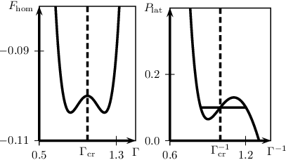
In the simulations we used a simple symmetric double well potential $F_{\mathrm{hom}}$ employing the parameters ${\Gamma_{\mathrm{cr}}=1},{F_{1}=F_{3}=0},{F_{0}=-0.1},{F_{2}=-0.24},{F_{4}=3.85}$. Figure 3 shows the free-energy density $F_{\mathrm{hom}}$, as is obtained for our choice of parameters, as well as the resulting pressure-area diagram calculated according to eq. (12) for homogeneous values of $\Gamma$. The two minima of $F_{\mathrm{hom}}$ correspond to two thermodynamically stable phases of different surfactant density. Within this simple model, the phases of higher and lower density can be identified with the liquid-condensed (LC) phase and the liquid-expanded (LE) phase, respectively.

For the disjoining pressure (5) we use the parameters ${n=3},{m=9}$ with ${A_{3}=3}$ and ${A_{9}=1}$ and set the remaining dimensionless numbers to $\mathrm{Ca}^{-1}=1,A=0.05,K=0.05,{\bf v_{0}}=0$.

Our goal is to investigate how the surfactant affects the formation of droplets. Therefore, as initial conditions, small random perturbations of the stationary homogeneous solution ${\hat{H}=1.2}$ and ${\hat{\Gamma}=0.82345}$ are used. Since $\partial\Pi(1.2)/\partial H<0$ this corresponds to a flat film, which would be unstable to droplet formation even in absence of any surfactant. The value of $\hat{\Gamma}$ is chosen as the position of the lower density minimum of $F_{\mathrm{hom}}$. Thus, we are simulating a thin film uniformly covered with surfactant in its lower density phase.

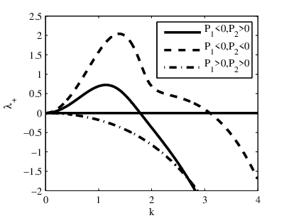
The parameter values specified above correspond to the case $P_{1}<0,P_{2}>0$ of the linear stability analysis. The wavenumber dependent growth rate $\mathrm{Re}(\lambda_{+}(k))$ is displayed in fig. 4. For comparison we also show $\mathrm{Re}(\lambda_{+}(k))$ for two different sets of $\hat{H},\hat{\Gamma}$. The first one where $P_{1}<0,P_{2}<0$ corresponds to the unstable fixed point $\hat{\Gamma}=\Gamma_{\mathrm{cr}}=1$ of $F_{\mathrm{hom}}$ and the same $\hat{H}=1.2$, whereas the other describes the stable case $P_{1}>0,P_{2}>0$ where again $\hat{\Gamma}=0.82345$ and $\hat{H}=0.9$. Now we are in position to determine numerically the maximal growth rates $\lambda_{+}(k_{\mathrm{max}})$ and the corresponding eigenvectors for the three parameter sets mentioned above. The calculations show that neither component of the eigenvectors is dominant. This indicates the coupling of the fields $H$ and $\Gamma$ even within the scope of linear theory.

Now we concentrate again on the initial condition $\hat{H}=1.2,\hat{\Gamma}=0.82345$. Time evolution of the nonlinear system in the one-dimensional case can be described as follows. In the beginning, spinodal dewetting and surfactant spinodal decomposition lead to rapid formation of liquid droplets and surfactant domains, the latter consisting of surfactant in a higher-density (LC) and a lower-density (LE) phase. Then a coarsening process sets in and drops of liquid coalesce while surfactant domains merge into larger ones. To visualize the coarsening of the liquid film and the surfactant density, we display the regions of negative curvature, which naturally indicate the location of drops and domains of high surfactant density, in a space-time diagram (see fig. 5). Figure 6 shows a snapshot of a later stage of the 1D simulation, where the few remaining high-density domains are clearly located on the largest liquid drops. Evidently, there is a strong correlation of $\Gamma$ and $H$. In the 2D case, morphology is similar. As can be seen in fig. 7, high-density domains are again located on the largest drops of liquid. To emphasise this correlation the contour line $\Gamma=1$ is drawn in the plot of the field $H$ (fig. 7 (a)) and vice versa. Like in the 1D simulation, drops, that are covered with surfactant in the low-density phase become smaller and smaller as $T$ increases, while drops covered with the high-density surfactant phase grow stronger during the coarsening. Obviously the surfactant has a sustaining effect on the drops, since the system energetically favours surfaces with lower surface tension.

We have modelled the dynamics of a thin liquid film covered with an insoluble surfactant in the vicinity of a phase transition. For that purpose we have incorporated a suitable free-energy functional for the surfactant into the two governing equations, which were derived within the lubrication approximation. Linear stability analysis revealed the interplay of surfactant spinodal decomposition and spinodal dewetting of the liquid film. Although result (23) for $k_{c}$ seems to imply that the liquid film and the surfactant are linearly decoupled, their time evolution is connected from onset. One- and two-dimensional simulations were presented, showing the decomposition of the surfactant into domains of material in thermodynamically stable phases. Droplets and domains show a strong spatial correlation resulting from the sustaining effect of the surfactant on droplets. The proposed model might serve as a starting point for further research on thin film dynamics with surfactant phase transitions and the related pattern formation. Also, further investigation is needed, to understand the role of the phase transition in Langmuir-Blodgett transfer systems. Thus, it will be necessary to solve the set of evolution equations subject to suitable boundary conditions.

This work was supported by the Deutsche Forschungsgemeinschaft within special research fund TRR 61. We thank L. F. Chi and M. Hirtz for helpful discussions.

References

- [1] Alexander Oron, Stephen H. Davis, and S. George Bankoff. Long-scale evolution of thin liquid films. Rev. Mod. Phys., 69(3):931–980, 1997.
- [2] P. G. de Gennes. Wetting: statics and dynamics. Rev. Mod. Phys., 57(3):827–863, 1985.
- [3] Len M. Pismen and Yves Pomeau. Disjoining potential and spreading of thin liquid layers in the diffuse-interface model coupled to hydrodynamics. Phys. Rev. E, 62(2):2480–2492, 2000.
- [4] Günter Reiter. Dewetting of thin polymer films. Phys. Rev. Lett., 68(1):75–78, 1992.
- [5] Michael Bestehorn and Kai Neuffer. Surface patterns of laterally extended thin liquid films in three dimensions. Phys. Rev. Lett., 87(4):046101, 2001.
- [6] S. M. Troian, X. L. Wu, and S. A. Safran. Fingering instability in thin wetting films. Phys. Rev. Lett., 62(13):1496–1499, Mar 1989.
- [7] R. V. Craster and O. K. Matar. Numerical simulations of fingering instabilities in surfactant-driven thin films. Phys. Fluids, 18(3):032103, 2006.
- [8] Vladimir M. Kaganer, Helmuth Möhwald, and Pulak Dutta. Structure and phase transitions in langmuir monolayers. Rev. Mod. Phys., 71(3):779–819, 1999.
- [9] O. Albrecht, H. Gruler, and E. Sackmann. Polymorphism of phospholipid monolayers. Journal de Physique, 39:301–313, 1978.
- [10] Eli Ruckenstein and Buqiang Li. Surface equation of state for insoluble surfactant monolayers at the air/water interface. J. Phys. Chem. B, 102(6):981–989, 1998.
- [11] Omar K. Matar and Sandra M. Troian. Linear stability analysis of an insoluble surfactant monolayer spreading on a thin liquid film. Phys. Fluids, 9(12):3645–3657, 1997.
- [12] M. Gleiche, L. F. Chi, and H. Fuchs. Nanoscopic channel lattices with controlled anisotropic wetting. Nature, 403:173–175, 2000.
- [13] K. Spratte, Li F. Chi, and H. Riegler. Physisorption instabilities during dynamic langmuir wetting. Europhys. Lett., 25(3):211–217, 1994.
- [14] X. Chen, S. Lehnert, M. Hirtz H., N. Lu, Fuchs, and Li F. Chi. Langmuir-blodgett patterning: A bottom-up way to build mesostructures over large areas. Acc. Chem. Res., 40(6):393–401, 2007.
- [15] Donald P. Gaver and James B. Grotberg. The dynamics of a localized surfactant on a thin film. J. Fluid Mech., 213(-1):127–148, 1990.
- [16] M. R. E. Warner, R. V. Craster, and O. K. Matar. Dewetting of ultrathin surfactant-covered films. Phys. Fluids, 14(11):4040–4054, 2002.
- [17] Z. Dagan and L. M. Pismen. Marangoni waves induced by a multistable chemical reaction on thin liquid films. J. Coll. Int. Sci., 99(1):215–225, 1984.
- [18] A. De Wit, D. Gallez, and C. I. Christov. Nonlinear evolution equations for thin liquid films with insoluble surfactants. Phys. Fluids, 6(10):3256–3266, 1994.
- [19] L. E. Scriven. Dynamics of a fluid interface equation of motion for newtonian surface fluids. Chem. Eng. Sci., 12(2):98–108, 1960.
- [20] H. A. Stone. A simple derivation of the time-dependent convective-diffusion equation for surfactant transport along a deforming interface. Phys. Fluids A, 2(1):111–112, 1990.
- [21] Rutherford Aris. Vectors, tensors and the basis equations of fluids mechanics. Dover, New-York, 1989.
- [22] A. W. Adamson. Physical Chemistry of Surfaces. Wiley Interscience, 1990.
- [23] John W. Cahn and John E. Hilliard. Free energy of a nonuniform system. i. interfacial free energy. Journal Chem. Phys., 28(2):258–267, 1958.
- [24] R. Evans. The nature of the liquid-vapour interface and other topics in the statistical mechaniocs of non-uniform, classical fluids Adv. Phys. 28(2):143–200, 1979.
- [25] L. D. Landau and E. M. Lifschitz. Statistische Physik, Teil 1. Akademie Verlag, Berlin, 1987.
- [26] L. D. Landau and E. M. Lifschitz. Hydrodynamik. Akademie Verlag, Berlin, 1991.
- [27] John P. Boyd. Chebyshev and Fourier Spectral Methods 2nd Edition. Dover, New-York, 2000.
- [28] William H. Press. Numerical Recipes in C. University Press, Cambridge, 1999.