跳到论文正文
W Papers独立论文阅读器 arXiv:0903.1719 论文正文 计算阅读时间 · 0%
引用这篇论文根据当前论文元数据生成,正式投稿前建议核对。


License: arXiv.org perpetual non-exclusive license
arXiv:0903.1719v1 [hep-ph] 10 Mar 2009

CPT-P003-2009

Mars 2009

Reduction of one-massless-loop with scalar boxes in n+2n+2 dimensions.

C. Bernicot a

a CPT, Luminy, CNRS
UMR 6207
Campus de Luminy, Case 907 - 13288 Marseille cedex 9, France.

All one-massless-loop Feynman diagrams could be written like a linear combination of scalar boxes, triangles an bubbles in nn dimensions plus rational terms. However, the four-point scalar integrals in n+2n+2 dimensions are free of infrared divergences. We are going to change the dimensions of the scalar boxes n→n+2n\rightarrow n+2 and the using of this degree of freedom to simplify the computation of coefficients of the decomposition.

version August 24, 2026

1 Introduction

Since many years, one have try to calculate analytically Feynman Diagrams. The aim is the computation of amplitudes and cross sections. In fact, at the LHC, we want to discover new physics and new particles like Higgs by the interaction of two protons. The background is constituted by many QCD reactions. So the knowlegde of this pone is necessary, if we want to detect a new particle. But the amplitudes depend to an unphysical energy, and this dependance decreases with the order of the development. So to have a good prediction, we have to calculate each reaction at NLO. At this time, all 2→22\rightarrow 2 and 2→32\rightarrow 3 processes are known at NLO, but it remains the 2→N2\rightarrow N, with N>3N>3. So we have to calculate one-loop diagrams with many ingoing legs.

Forty years ago, Passarino and Veltman gave a first method to reduce diagrams. This method is not really efficient and doesn’t use the mathematical symmetry of a loop, for example, unitarity. They showed that we can write a diagram like a linear combination of scalar integrals. Then since ten years, Bern and al. [1, 2, 3, 4] reduce diagrams thanks to unitarity. It simplifies computation. In 2004, Britto and al. [5, 6, 7, 8, 9] gave a very efficient method to calculate the coefficients in front of the four-point scalar integrals. Then, Mastrolia [10] found a way to express the coefficients in front of triangles. Recently Forde [11] in one hand and Papadopoulos and al. [12] in a other hand gave some algorithms to obtain directly the coefficients in front of the scalar massless boxes, triangles and bubbles. Finally, Kilgore [13] improves the Forde algorithms to a massive loop. But in this algorithm, less the scalar integrals have legs, more the coefficients are difficult to calculate because some free parameters appear. In fact, as they use unitarity and cuts, we need four cuts to define a loop momenta. But we have only three cuts (respectively two cuts) in a triangle (resp. in a bubble). So some free parameters remains.

In this paper, I would like to give a way to eliminate this degree of freedom in front of the triangles in a massless loop. Just after given some notations in the section 2, I would like to speak about the bases of scalar integrals in section 3 and to show that the classical base is not efficient, therefore I give a better base. Then, in section 4, I would like to give a way to find coefficients in front of triangles in this new bases. Finally I finish by an exemple in section 5: the four-photon amplitudes. For a massive loop more work are needed.

2 Notations

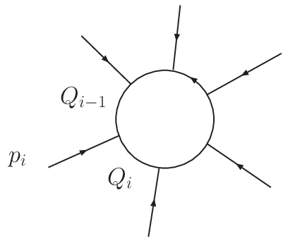
So in this first section we gave some notations. The purpose of this article is to study the decomposition of a one-massless loop Feynman diagram amplitude. So consider a one-loop diagram with NN ingoing legs (Fig. 1), we note it amplitude:

𝒜N=∫dn​Q​Num​(Q)D12​…​DN2,\displaystyle{\cal A}_{N}\ =\ \int d^{n}Q\frac{\textrm{Num}(Q)}{D_{1}^{2}...D_{N}^{2}}, (1)

with QQ the loop momentum in n=4−2​ϵn=4-2\epsilon dimensions and the denominator Di2=Qi2+i​λ=(Q+ri)2+i​λD_{i}^{2}\ =\ Q_{i}^{2}+i\lambda\ =\ \left(Q+r_{i}\right)^{2}+i\lambda. We decide to note the nn-dimensional vectors in capital letters and the 44-dimensional vectors in small letters. The −2​ϵ-2\epsilon part of the loop momentum is μ\mu. As the four and the −2​ϵ-2\epsilon parts Minkowski space are orthogonal, therefore the denominator “i” is written:

Di2=Qi2+i​λ=(qi+μ)2+i​λ=qi2+i​λ−μ2=di2−μ2.D_{i}^{2}\ =\ Q_{i}^{2}+i\lambda\ =\ \left(q_{i}+\mu\right)^{2}+i\lambda\ =\ q_{i}^{2}+i\lambda-\mu^{2}\ =\ d_{i}^{2}-\mu^{2}. (2)

“di2d_{i}^{2}” is the four dimensional part of the denominator “i”. The function Num​(Q)\textrm{Num}(Q) depends on the theory with described the loop. In classical gauge theory, this function is polynomial.

In particularly, we note INnI_{N}^{n} the amplitude of a one-loop diagram, with NN external legs, where all internal propagators are scalar:

INn=∫dn​Q​1D12​…​DN2.\displaystyle I_{N}^{n}\ =\ \int d^{n}Q\frac{1}{D_{1}^{2}...D_{N}^{2}}. (3)

We often call those amplitudes: scalar integrals. There are well-known and we can express them with explicit analytic expressions. We recall some of them in Appendix A. Moreover, we use oftentimes the kinematical matrix 𝒮i​j{\cal S}_{ij} and the Gram matrix Gi​jG_{ij}, defined (for a massless loop) by:

𝒮i​j=(qi−qj)2Gi​j= 2​pi.pj\displaystyle{\cal S}_{ij}\ =\ \left(q_{i}-q_{j}\right)^{2}\quad\quad G_{ij}\ =\ 2p_{i}.p_{j} (4)
Refer to caption
Figure 1: General structure of a loop.

3 The bases of decomposition

Now we assume a one-massless-loop Feynman diagram, described in a gauge theory by the amplitude (1)\left(\ref{ampliini}\right). The numerator of the amplitude is a polynomial function. This last point out is very importante to decompose the amplitude.

3.1 The classical base

As the loop are described in a standard gauge theory, therefore, the integrand of the amplitude is a rational function. We can expand it automatically in partial fractions. Each one gives a scalar integral. Therefore, we can write straightforward an amplitude like a linear combination of scalar integrals in nn dimensions:

𝒜N=∑i=1Nai​Iin+Rationnal terms+O⁡(ϵ).\displaystyle{\cal A}_{N}\ =\ \sum_{i=1}^{N}a_{i}I_{i}^{n}+\textrm{Rationnal terms}+O(\epsilon). (5)

Obviously the decomposition of an NN external-leg one-loop Feynman diagram uses scalar integrals with at most NN external legs. However, all those integrals {Iin,n∈[1..N]}\left\{I_{i}^{n},\ n\in[1..N]\right\} are not free. Indeed, we have the linear relation [14, 15]:

INn​(𝒮)=∑i,j=1N𝒮i​j−1​IN−1n​(𝒮−{i})i−(−1)N+1​(N−n−1)​det(G)det(𝒮)​INn+2​(𝒮),I_{N}^{n}\left({\cal S}\right)\ =\ \sum_{i,j=1}^{N}{\cal S}_{ij}^{-1}{I_{N-1}^{n}\left({\cal S}-\{i\}\right)}_{i}-(-1)^{N+1}\left(N-n-1\right)\frac{\det\left(G\right)}{\det\left({\cal S}\right)}I_{N}^{n+2}\left({\cal S}\right), (6)

where 𝒮−{i}{\cal S}-\{i\} is the kinematical matrix obtained by eliminate the column and the line number “i”. Moreover, we can show that the Gram determinant for N>5N>5 is equal to zero. So this last equation (6)\left(\ref{reductionint}\right) simplify:

{∀N>5,INn​(𝒮)=∑i,j=1N𝒮i​j−1​IN−1n​(𝒮−{i})iI5n​(𝒮)=∑i,j=15𝒮i​j−1​I4n​(𝒮−{i})i−2​ϵ​det(G)det(𝒮)​I5n+2​(𝒮).\displaystyle\left\{\begin{array}[]{l}\displaystyle\forall\ N>5,\ I_{N}^{n}\left({\cal S}\right)\ =\ \sum_{i,j=1}^{N}{\cal S}_{ij}^{-1}{I_{N-1}^{n}\left({\cal S}-\{i\}\right)}_{i}\\ \displaystyle I_{5}^{n}\left({\cal S}\right)\ =\ \sum_{i,j=1}^{5}{\cal S}_{ij}^{-1}{I_{4}^{n}\left({\cal S}-\{i\}\right)}_{i}-2\epsilon\ \frac{\det\left(G\right)}{\det\left({\cal S}\right)}I_{5}^{n+2}\left({\cal S}\right).\end{array}\right.

So we see easily that in the leading order in ϵ\epsilon, the reduction (6)\left(\ref{reductionint}\right) simplify (as the loop is massless, we don’t need tadpoles to decompose the loop):

𝒜N=∑i=24ai​Iin+O⁡(ϵ).\displaystyle{\cal A}_{N}\ =\ \sum_{i=2}^{4}a_{i}I_{i}^{n}+O(\epsilon). (9)

We need only scalar boxes, triangles, bubbles and rational terms to generate all the one-massless-loop Feynman diagrams. Generally we call the scalar function part: the analytic part and the rational terms the rational part. The call “analytic part” comes from fact that they contains polylogarithm functions of Mandelstam variables. The rational terms are studied in [16, 17]. But we are going to see, that this base ℬ={I2n,…​I4n}{\cal B}\ =\ \{I_{2}^{n},...I_{4}^{n}\} is not efficient.

𝒜N=∑i\displaystyle{\cal A}_{N}\ =\ \sum_{i}\ ai​[Uncaptioned image]n+bi​[Uncaptioned image]n+ci​[Uncaptioned image]n+\displaystyle a_{i}\parbox{56.9055pt}{\includegraphics[width=56.9055pt]{I4m4.eps}}^{n}+b_{i}\parbox{56.9055pt}{\includegraphics[width=56.9055pt]{I4m3.eps}}^{n}+c_{i}\parbox{56.9055pt}{\includegraphics[width=56.9055pt]{I4m2A.eps}}^{n}+
+\displaystyle+ di​[Uncaptioned image]n+ei​[Uncaptioned image]n+fi​[Uncaptioned image]n+\displaystyle d_{i}\parbox{56.9055pt}{\includegraphics[width=56.9055pt]{I4m2B.eps}}^{n}+e_{i}\parbox{56.9055pt}{\includegraphics[width=56.9055pt]{I4m1.eps}}^{n}+f_{i}\parbox{56.9055pt}{\includegraphics[width=56.9055pt]{I4m0.eps}}^{n}+
+\displaystyle+ gi​[Uncaptioned image]n+hi​[Uncaptioned image]n+ii​[Uncaptioned image]n+\displaystyle g_{i}\parbox{56.9055pt}{\includegraphics[width=56.9055pt]{I3m3.eps}}^{n}+h_{i}\parbox{56.9055pt}{\includegraphics[width=56.9055pt]{I3m2.eps}}^{n}+i_{i}\parbox{56.9055pt}{\includegraphics[width=56.9055pt]{I3m1.eps}}^{n}+
+\displaystyle+ ji​[Uncaptioned image]n+Rational Terms\displaystyle j_{i}\parbox{56.9055pt}{\includegraphics[width=56.9055pt]{I2m1.eps}}^{n}+\textrm{Rational Terms}

The acknowledge of the coefficients {ai,…​ji}\{a_{i},...j_{i}\} and the rational terms is enough to reconstruction all the amplitude. This base ℬ={I2n,…​I4n}{\cal B}\ =\ \{I_{2}^{n},...I_{4}^{n}\} is the most obvious, the canonical base, but not the more efficient. It is the subject of the next subsection.

3.2 The problems of this base ℬ{\cal B}

The base of decomposition ℬ={I2n,…​I4n}{\cal B}\ =\ \{I_{2}^{n},...I_{4}^{n}\} has at least two problems.

The first comes from divergences. Indeed, the four-point functions are constituted by finite terms and infrared divergent terms, the three-point functions are infrared divergent and the bubbles: UV divergent. So three and four-point functions could have infrared divergences. Therefore, with the base ℬ{\cal B}, we don’t have separate explicitly the infrared, ultraviolet and finite structure. It could forget some compensations and it is not easy to found them. For instance, consider a loop without infrared divergences, therefore we can have three and four-point functions and not explicite compensations, this implies some numerical instabilities.

The second problem concerns the famous Gram determinant. The reduction gives some negative powers of Gram determinants in front of the four-point functions. This determinant is spurious, because it could be equal to zero but this divergence is not physic, it has no physical explanation. Indeed, there is some unexplicit compensations to eliminate those determinants.

Those two problems give the base ℬ{\cal B} not efficient. So we have to find an other base.

3.3 A better base

The main problem is the blend of infrared, ultraviolet and finite parts and in particularly, it should be genius if we could separate the infrared and the finite part of the four-point scalar functions. We could do it just by the application of the formula (6)\left(\ref{reductionint}\right) to the four-point scalar integrals:

I4n​(𝒮)=∑i,j=14𝒮i​j−1​I3n​(𝒮−{i})i−(1+2​ϵ)​det(G)det(𝒮)​I4n+2​(𝒮).I_{4}^{n}\left({\cal S}\right)\ =\ \sum_{i,j=1}^{4}{\cal S}_{ij}^{-1}{I_{3}^{n}\left({\cal S}-\{i\}\right)}_{i}-\left(1+2\epsilon\right)\frac{\det\left(G\right)}{\det\left({\cal S}\right)}I_{4}^{n+2}\left({\cal S}\right). (10)

The four-point scalar functions in n+2n+2 dimensions are totally finite and well-known, we recall them in Appendix A. Moreover (10)\left(\ref{equredcution}\right) see us that it appears one Gram determinant in the numerator of the coefficients in front of the four-point functions. So with (10)\left(\ref{equredcution}\right), we reduce one time the problem of the Gram determinant, but we don’t eliminate all the problem. So we conclude that the base ℬ′={I2n,I3n,I4n+2}{\cal B}^{{}^{\prime}}\ =\ \left\{I_{2}^{n},I_{3}^{n},I_{4}^{n+2}\right\} is better than ℬ{\cal B}. It remains to calculate the coefficients in front of each scalar integral.

𝒜N=∑i\displaystyle{\cal A}_{N}\ =\ \sum_{i}\ ai′[Uncaptioned image]n+2+bi′[Uncaptioned image]n+2+ci′[Uncaptioned image]n+2+\displaystyle a_{i}^{{}^{\prime}}\parbox{56.9055pt}{\includegraphics[width=56.9055pt]{I4m4.eps}}^{n+2}+b_{i}^{{}^{\prime}}\parbox{56.9055pt}{\includegraphics[width=56.9055pt]{I4m3.eps}}^{n+2}+c_{i}^{{}^{\prime}}\parbox{56.9055pt}{\includegraphics[width=56.9055pt]{I4m2A.eps}}^{n+2}+
+\displaystyle+ di′[Uncaptioned image]n+2+ei′[Uncaptioned image]n+2+fi′[Uncaptioned image]n+2+\displaystyle d_{i}^{{}^{\prime}}\parbox{56.9055pt}{\includegraphics[width=56.9055pt]{I4m2B.eps}}^{n+2}+e_{i}^{{}^{\prime}}\parbox{56.9055pt}{\includegraphics[width=56.9055pt]{I4m1.eps}}^{n+2}+f_{i}^{{}^{\prime}}\parbox{56.9055pt}{\includegraphics[width=56.9055pt]{I4m0.eps}}^{n+2}+
+\displaystyle+ gi′[Uncaptioned image]n+hi′[Uncaptioned image]n+ii′[Uncaptioned image]n+\displaystyle g_{i}^{{}^{\prime}}\parbox{56.9055pt}{\includegraphics[width=56.9055pt]{I3m3.eps}}^{n}+h_{i}^{{}^{\prime}}\parbox{56.9055pt}{\includegraphics[width=56.9055pt]{I3m2.eps}}^{n}+i_{i}^{{}^{\prime}}\parbox{56.9055pt}{\includegraphics[width=56.9055pt]{I3m1.eps}}^{n}+
+\displaystyle+ ji[Uncaptioned image]n+Rationnal Terms.\displaystyle j_{i}\parbox{56.9055pt}{\includegraphics[width=56.9055pt]{I2m1.eps}}^{n}+\textrm{Rationnal Terms}.

The ultraviolet divergences are carried out by the scalar bubbles, whereas the infrared structures are contained by the one and two-external-mass scalar triangles, but the finite structure are the four-point functions and the three-external-mass scalar triangle. So this decomposition partitions the amplitudes over the three kind of analytic structure without covering.

We will see that this partition is very interesting. It eliminates many subtil compensations. And the result that we are going to show is that if the loop has no infrared divergences, so the decomposition has no infrared structure. The extension of this result to the ultraviolet one is not so easy.

4 Coefficients in front of boxes and triangles in the base ℬ′={I2n,I3n,I4n+2}{\cal B}^{{}^{\prime}}=\left\{I_{2}^{n},I_{3}^{n},I_{4}^{n+2}\right\}

Now we are going to calculate the coefficients {ai′,…,ji}\{a_{i}^{{}^{\prime}},...,j_{i}\} in this new base ℬ′={I2n,I3n,I4n+2}{\cal B}^{{}^{\prime}}=\left\{I_{2}^{n},I_{3}^{n},I_{4}^{n+2}\right\}. In this section, we give the method to calculate the coefficients of the four and three-point functions. The ones in front of bubbles will be given in an other paper.

4.1 Coefficients of four-point functions.

To transform the base ℬ={I2n,I3n,I4n}{\cal B}\ =\ \left\{I_{2}^{n},I_{3}^{n},I_{4}^{n}\right\} to the base ℬ′={I2n,I3n,I4n+2}{\cal B}^{{}^{\prime}}\ =\ \left\{I_{2}^{n},I_{3}^{n},I_{4}^{n+2}\right\}, we have just to apply the formula (10)\left(\ref{equredcution}\right) to the first base. So keeping only the four-point scalar function part, the transformation gives us:

ai​I4n→−(4−n−1)​det(G)det(𝒮)​ai​I4n+2.a_{i}I_{4}^{n}\ \rightarrow\ -\left(4-n-1\right)\frac{\det\left(G\right)}{\det\left({\cal S}\right)}a_{i}I_{4}^{n+2}. (11)

So, we obtain the bounding equation:

ai′=−(4−n−1)det(G)det(𝒮)ai,a_{i}^{{}^{\prime}}\ =\ -\left(4-n-1\right)\frac{\det\left(G\right)}{\det\left({\cal S}\right)}a_{i}, (12)

where GG (respectively 𝒮\cal S) are the Gram matrix (resp. kinematical matrix) of the four-point scalar function. The coefficient aia_{i} is given directly by the unitarity-cut method [7, 18]. We recall it, for example, consider a loop with NN ingoing legs described by the amplitude (1)\left(\ref{ampliini}\right) and, we want the coefficient in front of the box obtained by pinching the denominators of the initial loop except the four ones called “a,b,ca,b,c” and “dd”. Therefore, the unitary cuts give us directly the coefficient by the limit:

ai=limda2,db2,dc2,dd2→0Num​(q)​da2​db2​dc2​dd2d12​…​dN2,a_{i}\ =\ \lim_{d_{a}^{2},d_{b}^{2},d_{c}^{2},d_{d}^{2}\rightarrow 0}\frac{\textrm{Num}\left(q\right)d_{a}^{2}d_{b}^{2}d_{c}^{2}d_{d}^{2}}{d_{1}^{2}...d_{N}^{2}}, (13)

where di2d_{i}^{2} represents the four-dimensional part of the denominator Di2D_{i}^{2}: di2=qi2+i​λd_{i}^{2}=q_{i}^{2}+i\lambda (eq. 2). To obtain this limit we have just to solve the system {i∈[a..d],di2=0}\{i\in[a..d],d_{i}^{2}=0\}. The loop momentum is a four-dimensional vector, so we write it like a linear combination of four four-dimensional vectors (for example external ingoing legs). The system is linear, with four equations and four variables (four parameters of the linear combination of the loop momentum), so we can solve it exactly, and we explicite the momentum of the loop. We note q0q_{0} this momentum. This process is explained in [5, 7, 12, 19, 20].

4.2 Coefficients of three-point functions.

In this subsection we use the Forde results and the Forde formalism given in [11]. Here we give the method to find the coefficient in front the three-point functions, assuming that the four-point functions are in n+2n+2 dimensions. To simplify the proof, we use an amplitude with four external legs:

𝒜4=∫dn​Q​Num​(Q)D12​D22​D32​D42,{\cal A}_{4}\ =\ \int d^{n}Q\frac{\textrm{Num}\left(Q\right)}{D_{1}^{2}D_{2}^{2}D_{3}^{2}D_{4}^{2}}, (14)

which we decompose on the base ℬ′={I2n,I3n,I4n+2}{\cal B}^{{}^{\prime}}=\left\{I_{2}^{n},I_{3}^{n},I_{4}^{n+2}\right\} and rational terms:

𝒜4=−a​det(G)det(𝒮)​I4n+2+∑i=14Ti​I3,in+∑i=12γi​I2n+rationnal terms.{\cal A}_{4}\ =\ -a\frac{\det\left(G\right)}{\det\left({\cal S}\right)}I_{4}^{n+2}+\sum_{i=1}^{4}T_{i}I_{3,i}^{n}+\sum_{i=1}^{2}\gamma_{i}I_{2}^{n}+\textrm{rationnal terms}. (15)

With the last subsection, we can compute, very easily the coefficient in front of the four-point function, we know a=Num​(q0)a=\textrm{Num}(q_{0}), where q0q_{0} is the solve of the linear system {∀i∈[1..4],di2=0\left\{\forall i\in[1..4],\ d_{i}^{2}=0\right. given by the four cuts. Now we want to calculate the coefficients in front triangles. We are going to use the fact that [14, 15]:

−det(G)det(𝒮)​I4n+2=∫dn​Q​1−∑i=14bi​Di2D12​D22​D32​D42,-\frac{\det\left(G\right)}{\det\left({\cal S}\right)}I_{4}^{n+2}\ =\ \int d^{n}Q\frac{1-\sum_{i=1}^{4}b_{i}D_{i}^{2}}{D_{1}^{2}D_{2}^{2}D_{3}^{2}D_{4}^{2}}, (16)

where bi=∑j=14𝒮i​j−1b_{i}=\sum_{j=1}^{4}{\cal S}_{ij}^{-1}. The amplitude becomes:

𝒜4=∫dn​Q​Num​(Q)D12​D22​D32​D42=\displaystyle{\cal A}_{4}\ =\ \int d^{n}Q\frac{\textrm{Num}\left(Q\right)}{D_{1}^{2}D_{2}^{2}D_{3}^{2}D_{4}^{2}}\ = Num​(q0)​∫dn​Q​1−∑i=14bi​Di2D12​D22​D32​D42\displaystyle\ \textrm{Num}\left(q_{0}\right)\int d^{n}Q\frac{1-\sum_{i=1}^{4}b_{i}D_{i}^{2}}{D_{1}^{2}D_{2}^{2}D_{3}^{2}D_{4}^{2}}
+∑i=14Ti∫dnQDi2D12​D22​D32​D42+∑i=12γiI2n+Rationnal Terms.\displaystyle+\sum_{i=1}^{4}T_{i}\int d^{n}Q\frac{D_{i}^{2}}{D_{1}^{2}D_{2}^{2}D_{3}^{2}D_{4}^{2}}+\sum_{i=1}^{2}\gamma_{i}I_{2}^{n}+\textrm{Rationnal Terms}. (17)

For example, we assume that we want to calculate the coefficient in front of the three-point scalar function obtained by pinching the propagator number 1. So we apply, in the last equation (17)\left(\ref{III}\right), the linear application “Disc2,3,4\textrm{Disc}_{2,3,4}”, which cuts the three propagators 2,3 and 4 in four dimensions:

Disc2,3,4​𝒜4=Disc2,3,4​∫dn​Q​Num​(Q)D12​D22​D32​D42=\displaystyle\textrm{Disc}_{2,3,4}{\cal A}_{4}\ =\ \textrm{Disc}_{2,3,4}\int d^{n}Q\frac{\textrm{Num}\left(Q\right)}{D_{1}^{2}D_{2}^{2}D_{3}^{2}D_{4}^{2}}\ = Num​(q0)​Disc2,3,4​∫dn​Q​1−∑i=14bi​Di2D12​D22​D32​D42\displaystyle\ \textrm{Num}\left(q_{0}\right)\textrm{Disc}_{2,3,4}\int d^{n}Q\frac{1-\sum_{i=1}^{4}b_{i}D_{i}^{2}}{D_{1}^{2}D_{2}^{2}D_{3}^{2}D_{4}^{2}}
+∑i=14TiDisc2,3,4∫dnQDi2D12​D22​D32​D42.\displaystyle+\sum_{i=1}^{4}T_{i}\ \textrm{Disc}_{2,3,4}\int d^{n}Q\frac{D_{i}^{2}}{D_{1}^{2}D_{2}^{2}D_{3}^{2}D_{4}^{2}}. (18)

We keep on only the three and four-point functions. The application “Disc2,3,4\textrm{Disc}_{2,3,4}” inputs the three propagators d22,d32d_{2}^{2},d_{3}^{2} and d42d_{4}^{2} on-shell. As we keep only the four-dimensional part in the numerator, because we want the coefficient in front of the scalar integrals. Indeed, the −2​ϵ-2\epsilon dimensional part of the loop momentum in the numerator give the rational terms [16]. Therefore (18)\left(\ref{IIII}\right) becomes:

∫dn​Q​Num​(Q)D12​δ​(2,3,4)=\displaystyle\int d^{n}Q\ \frac{\textrm{Num}\left(Q\right)}{D_{1}^{2}}\ \delta\left(2,3,4\right)\ = Num​(q0)​∫dn​Q​1−b1​D12D12​δ​(2,3,4)+T1​∫dn​Q​δ​(2,3,4),\displaystyle\ \textrm{Num}\left(q_{0}\right)\int d^{n}Q\frac{1-b_{1}D_{1}^{2}}{D_{1}^{2}}\delta\left(2,3,4\right)+T_{1}\int d^{n}Q\ \delta\left(2,3,4\right), (19)

where δ⁡(2,3,4)=δ⁡(d22)​δ​(d32)​δ​(d42)\delta\left(2,3,4\right)=\delta\left(d_{2}^{2}\right)\delta\left(d_{3}^{2}\right)\delta\left(d_{4}^{2}\right). In this step we use the Forde Formalism [11]. As we have only three cuts, we have only three equations. We write again the loop momentum like a linear combination of four four-dimensional vectors {K3bμ,K4bμ,⟨K3b​γμ​K4b⟩,⟨K4b​γμ​K3b⟩}\left\{{K_{3}^{b}}^{\mu},{K_{4}^{b}}^{\mu},{\langle}K_{3}^{b}\gamma^{\mu}K_{4}^{b}{\rangle},{\langle}K_{4}^{b}\gamma^{\mu}K_{3}^{b}{\rangle}\right\}, where K3bμ{K_{3}^{b}}^{\mu} and K4bμ{K_{4}^{b}}^{\mu} are light-like vectors defined in the Appendix B. But as we have only three equations, therefore, we can explicit only three parameters over four of the linear combination of the loop momentum. The one, which it remains, is noted “c”. According to [11], q3q_{3} becomes:

q3​(c)=α04​K3bμ+α03​K4bμ+c2​⟨K3b​γμ​K4b⟩+α03​α042​c​⟨K4b​γμ​K3b⟩.q_{3}(c)\ =\ \alpha_{04}{K_{3}^{b}}^{\mu}+\alpha_{03}{K_{4}^{b}}^{\mu}+\frac{c}{2}{\langle}K_{3}^{b}\gamma^{\mu}K_{4}^{b}{\rangle}+\frac{\alpha_{03}\alpha_{04}}{2c}{\langle}K_{4}^{b}\gamma^{\mu}K_{3}^{b}{\rangle}. (20)

where all αi​j\alpha_{ij} and vectors KiK_{i} are explained in Forde paper [11] and recalled in the Appendix B. Moreover, we use the spinor notations introduced in [21]. Now we change the variables of integration and do the integrations over the three delta functions. We obtain:

∫d​c​Jc​Num​(c)D1​(c)2=Num​(q0)​∫d​c​Jc​1−b1​D12​(c)D12​(c)+T1​∫d​c​Jc.\ \int dc\ J_{c}\ \frac{\textrm{Num}\left(c\right)}{D_{1}(c)^{2}}\ =\ \textrm{Num}\left(q_{0}\right)\int dc\ J_{c}\frac{1-b_{1}D_{1}^{2}(c)}{D_{1}^{2}(c)}+T_{1}\int dc\ J_{c}. (21)

If we want to calculate the coefficient of the three point function, we have just to solve the equation:

1−b1​d12​(c0)= 0,1-b_{1}d_{1}^{2}\left(c_{0}\right)\ =\ 0, (22)

where D12=d12−μ2D_{1}^{2}=d_{1}^{2}-\mu^{2} (eq. 2). We put those II solves c0(i)c_{0}^{(i)} in the equation (21)\left(\ref{OPQ}\right) and we obtain the result.

Résultat 4.1

In the base ℬ′{\cal B}^{{}^{\prime}}, the coefficient in front of the scalar integrals I3,1nI_{3,1}^{n} is:

T1=b1​∑i=1INum​(c0(i)),T_{1}\ =\ b_{1}\sum_{i=1}^{I}\textrm{Num}\left(c_{0}^{(i)}\right), (23)

where c0c_{0} is the solve of the equation (22)\left(\ref{equationXXX}\right). For the other triangles, we have just to permute the cut propagators and the parameter bib_{i}.

Here we see one of the interest of the base ℬ′{\cal B}^{{}^{\prime}} rather than the base ℬ{\cal B}. Indeed, not only the base ℬ′{\cal B}^{{}^{\prime}} separate the infrared, ultraviolet and the finite parts but also the coefficients in front of scalar triangles are very simple to computed. There are no longer problems to obtain the free parameters, it is given by the equation (22)\left(\ref{equationXXX}\right). The solve of this equation is often obvious. In the last example, if one of the legs p3p_{3} or p4p_{4} is massless therefore, the solve is zero: c0=0c_{0}=0.

To improve the computation in this base ℬ′{\cal B}^{{}^{\prime}}, we are going to give some rules. With them, we are going to know directly, without computation, the null coefficients in front of triangles.

4.3 Infrared Divergences

Proposition 4.2

Consider the decomposition of an one-massless-loop Feynman diagram on the base ℬ′={I2n,I3n,I4n+2}{\cal B}^{{}^{\prime}}\ =\ \left\{I_{2}^{n},I_{3}^{n},I_{4}^{n+2}\right\}. We assume that this diagram has no infrared (soft or collinear) divergence. Therefore the coefficients in front of the scalar one or two-external-massive-leg triangles are zero.

Proof : We can give an analytical proof, but with some arguments of reduction, the proof is obvious.
Consider a one-loop-massless diagram free of IR divergences. The reduction by standard methods gives some sub-diagrams by pinching propagators. But those reduction cannot create infrared divergences. Indeed the pinched propagator plus the two-adjacent legs give a massive-external leg, which eliminates all infrared divergences around it. After the reduction, we obtain three-point sub-diagrams and the “finite” part of four-point scalar integrals. Since the three-point sub-diagrams are free of IR divergences, they cannot be expressed in term of one mass/two mass three-point scalar integrals and so the coefficients in front of them are zero.   ⊓\sqcap⊔\sqcup

We can improve this result and consider a diagram with infrared divergences.

Proposition 4.3

Consider the decomposition of an one-massless-loop Feynman diagram, with a soft divergence on the propagator number “i”, on the base ℬ′={I2n,I3n,I4n+2}{\cal B}^{{}^{\prime}}\ =\ \left\{I_{2}^{n},I_{3}^{n},I_{4}^{n+2}\right\}. The coefficients in front of the one-external and two-external-massive-leg triangles are zero except the one which corresponds to the one-external-massive-leg triangle whom the external-massive-leg is opposite to the propagator number “i”:

[Uncaptioned image]=∑iai​I4n+2i+b⁡([Uncaptioned image])+∑ici​I2ni\parbox{56.9055pt}{\includegraphics[width=56.9055pt]{regleinfrouge1.eps}}=\sum_{i}a_{i}{I_{4}^{n+2}}_{i}+b\ \left(\parbox{56.9055pt}{\includegraphics[width=56.9055pt]{regleinfrouge2.eps}}\right)+\sum_{i}c_{i}{I_{2}^{n}}_{i}
Proposition 4.4

Consider the decomposition of a one-massless-loop Feynman diagram, with a collinear divergence on the external leg “i”, on the base {I2n,I3n,I4n+2}\left\{I_{2}^{n},I_{3}^{n},I_{4}^{n+2}\right\}. The coefficients in front the one-external and two-external-massive-leg triangles are zero except the ones which correspond to the triangles, whom the leg number “i” doesn’t belong to an external mass:

[Uncaptioned image]=∑iai​I4n+2i+∑jbj​([Uncaptioned image])j+∑ici​I2ni\parbox{56.9055pt}{\includegraphics[width=56.9055pt]{reglecolineaire1.eps}}=\sum_{i}a_{i}\ {I_{4}^{n+2}}_{i}+\sum_{j}b_{j}\ \left(\parbox{56.9055pt}{\includegraphics[width=56.9055pt]{reglecolineaire2.eps}}\right)_{j}+\sum_{i}c_{i}\ {I_{2}^{n}}_{i}

Proof : The proofs are the same like the first proposition 4.2. The external mass regular the infrared divergences. Therefore all three-point sub-diagrams have a null coefficient except which one preserves the divergence.   ⊓\sqcap⊔\sqcup

Remark: In a loop, only photons, gluons or scalars create some divergent propagators. Indeed a fermion propagator has a numerator and this numerator compensate all infrared divergences.

If we decide to decompose a one-massless-loop Feynman diagram on the base ℬ′={I2n,I3n,I4n+2}{\cal B}^{{}^{\prime}}\ =\ \left\{I_{2}^{n},I_{3}^{n},I_{4}^{n+2}\right\}, using this last remark we deduce straightforward the three-point scalar integrals which have a null or non-null coefficients.

5 An Exemple: the four-photon amplitudes

We are going to calculate rapidly the helicity amplitudes of the four-photon amplitudes in QED for example, and in QED, scalar QED and supersymmetric QED 𝒩=1{}^{\cal N}=1. All the result are given in [22, 23, 24, 25, 26, 27, 28, 29, 30, 31], but we are going to found the results.

The four-photon amplitudes γ1+γ2+γ3+γ4→0\gamma_{1}+\gamma_{2}+\gamma_{3}+\gamma_{4}\rightarrow 0 in QED are null at tree order. The first non null order is the one-loop order. Therefore, the amplitude is six one-massless-loop diagrams with four photons ingoing in a loop of fermions. So the decomposition of the amplitude on the base ℬ′{\cal B}^{{}^{\prime}} is:

𝒜4=∑σ⁡(1,2,3,4)(a′I4n+2(σ)+b′I3n(σ)+cI2n(σ))+rationnal terms.{\cal A}_{4}\ =\ \sum_{\sigma(1,2,3,4)}\ \left(a^{{}^{\prime}}I_{4}^{n+2}\left(\sigma\right)+b^{{}^{\prime}}I_{3}^{n}\left(\sigma\right)+cI_{2}^{n}\left(\sigma\right)\right)+\textrm{rationnal terms}. (24)

However with the last subsection, as the loop is a fermion loop, therefore, there are no infrared divergence so b=0b=0. The decomposition becomes:

𝒜4=∑σ⁡(1,2,3,4)(a′I4n+2(σ)+cI2n(σ))+rationnal terms.{\cal A}_{4}\ =\ \sum_{\sigma(1,2,3,4)}\ \left(a^{{}^{\prime}}I_{4}^{n+2}\left(\sigma\right)+cI_{2}^{n}\left(\sigma\right)\right)+\textrm{rationnal terms}. (25)

a′a^{{}^{\prime}} is obtained by the equation (12)\left(\ref{coef4}\right):

a′=(1−2ϵ)det(G)det(𝒮)a,a^{{}^{\prime}}\ =\ (1-2\epsilon)\frac{\det(G)}{\det({\cal S})}\ a, (26)

where “aa” is given by unitary-cut. If all photons have a positive or a negative helicity therefore, at least two adjacent photons have the same helicity, and as the loop is massless therefore the coefficient is null. We explain it in [20]. We have the same argument if three photons have the same helicity:

a(++++)=a(−+++)= 0.a(++++)\ =\ a(-+++)\ =\ 0. (27)

.

If we have two positive-helicity photons and two negative-helicity photons therefore the coefficient is non null only if the helicities ingoing alternately in the loop. The non null coefficient corresponds to the scalar integrals I4n+2​(1+,2−,3+,4−)I_{4}^{n+2}\left(1^{+},2^{-},3^{+},4^{-}\right). The argument in this integrals gives the order in which the photon ingoing to the loop. We alternate the negative and the positive helicity photons. With some calculation with find directly:

a(−+−+)=−e4⟨12⟩[12][34]⟨34⟩t2+u2sa(-+-+)\ =\ -e^{4}\frac{\langle 12\rangle}{[12]}\frac{[34]}{\langle 34\rangle}\frac{t^{2}+u^{2}}{s} (28)

To compute the rational terms and the coefficients of bubbles we need other methods. In [24, 25, 26, 27, 28, 29, 30, 31], we find:

𝒜4(++++)\displaystyle\displaystyle{\cal A}_{4}(++++)\ = 8​i​α2​[12]​[34]⟨12⟩​⟨34⟩+O⁡(ϵ),\displaystyle=\ \displaystyle 8i\alpha^{2}\frac{[12][34]}{\langle 12\rangle\langle 34\rangle}+O(\epsilon), (29)
𝒜4(−+++)\displaystyle\displaystyle{\cal A}_{4}(-+++)\ = 8​i​α2​[34]​[231]⟨34⟩​⟨231⟩+O⁡(ϵ),\displaystyle=\ \displaystyle 8i\alpha^{2}\frac{[34][231]}{\langle 34\rangle\langle 231\rangle}+O(\epsilon), (30)
𝒜4(−−++)\displaystyle\displaystyle{\cal A}_{4}(--++)\ =−8​i​α2​⟨12⟩[12]​[34]⟨34⟩​{1+t2+u2s​I4n+2​(1324)+t−us​(I2n​(u)−I2n​(t))}+O⁡(ϵ).\displaystyle=\ \displaystyle-8i\alpha^{2}\frac{\langle 12\rangle}{[12]}\frac{[34]}{\langle 34\rangle}\left\{1+\frac{t^{2}+u^{2}}{s}I_{4}^{n+2}(1324)+\frac{t-u}{s}\left(I_{2}^{n}(u)-I_{2}^{n}(t)\right)\right\}+O\left(\epsilon\right). (31)

The definition of each scalar integrals are given in Appendix A. In the last helicity, the coefficients in front of bubbles are non null. They carried out ultraviolet divergences, but the amplitude is free of those divergence. But the soustraction of two bubbles compensate and those divergence disappear. We can extend those results to the six-photon amplitudes. All the results are given in [30, 31].

6 Conclusion

In this paper, we suggest a way to decompose a one-massless-loop Feynman diagram.

As the other methods of reduction, we decompose an amplitude like a linear combination of scalar integrals. But contrary to the methods already existing, here we use the scalar boxes in n+2n+2 dimensions. Thanks to this transformation, we win a degree of freedom which simplify the computation of the coefficients in front of the scalar triangles.

But it remains works to finish the method. Indeed, we have to incorpore the computation of the coefficients in front of bubbles and rational terms. But as the example of the four-photon amplitudes shows, the bound between the amplitude and the ultraviolet divergences is not so simple as the one with the infrared divergences.

Acknowledgements

I want to thank T. Binoth, G. Heinrich and P. Mastrolia for collaboration during the early stages of this work and for useful discussions. I would like to thank very much the CPT (Centre de Physique Théorique, Luminy, France) to welcome me during this year.

Appendix A Scalar integrals

In this appendix, for sake of completeness, the definition of master massless integrals used in this paper is recalled, more details can be found in [32]. We also give det(G)\det(G) the determinant of the Gram matrix Gi​j=2​pi.pjG_{ij}=2p_{i}.p_{j} built with the external four momentum and det(S)\det(S) the determinant of the kinematical S-matrix defined by Si​j=(qj−qi)2S_{ij}=\left(q_{j}-q_{i}\right)^{2} where the qiq_{i} are the four dimensional momentum flowing in the propagators. All was explain in section 2, but we remember the draw.

Refer to caption
Figure 2: General structure of a loop.

Moreover, we are going to use the dilogarithm function defined by [33]:

Li2(x)=−∫01dtln⁡(1−x​t)t.\textrm{Li}_{2}(x)\ =\ -\int_{0}^{1}dt\ \frac{\ln(1-xt)}{t}. (A.1)

In [33], we find many formulae using those dilogaritms. We have to be careful, the Mandelstam variables could be negative. They are in the arguments of the dilogarithm, so to solve the problem of the Riemann sheet of the logarithm we use the analytic continuation by adding a small imaginary part, the prescription is:

s→s+i​λ,with​λ>0.s\rightarrow s+i\lambda,\textrm{with}\ \lambda>0. (A.2)

And, all the scalar integrals must be multiplied by the angular integral:

rΓ=Γ⁡(1+ϵ)​Γ​(1−ϵ)2Γ⁡(1−2​ϵ).r_{\Gamma}\ =\frac{\Gamma(1+\epsilon)\Gamma(1-\epsilon)^{2}}{\Gamma(1-2\epsilon)}. (A.3)

A.1 Two-point Function.

[Uncaptioned image]s=s12=s34\displaystyle\parbox{71.13188pt}{\includegraphics[width=71.13188pt]{I2pappendix.eps}}\quad\quad\quad\quad\quad\quad\quad\quad s=s_{12}=s_{34}
𝒮2=(0ss0).\displaystyle{{\cal S}_{2}}=\begin{pmatrix}0&s\\ s&0\end{pmatrix}. (A.4)

The determinants are given by:

det(S2)=−s2\displaystyle\det\left(S_{2}\right)\ =\ -s^{2} (A.5)
det(G2)=s.\displaystyle\det\left(G_{2}\right)\ =\ s. (A.6)

The two-point function in nn dimensions is:

I2n​(s)=1ϵ⁡(1−2​ϵ)​(−s)−ϵ=1ϵ−ln⁡(−s)+2+O⁡(ϵ),I_{2}^{n}\left(s\right)\ =\ \displaystyle\frac{1}{\epsilon(1-2\epsilon)}\left(-s\right)^{-\epsilon}\ =\ \frac{1}{\epsilon}-\ln\left(-s\right)+2+O\left(\epsilon\right), (A.7)

and in n+2n+2 dimensions :

I2n+2​(s)=−12​ϵ​(1−2​ϵ)​(3−2​ϵ)​(−s)1−ϵ.I_{2}^{n+2}\left(s\right)\ =\ \displaystyle-\frac{1}{2\epsilon(1-2\epsilon)(3-2\epsilon)}\left(-s\right)^{1-\epsilon}. (A.8)

A.2 One-external-massive-leg three-point Function.

[Uncaptioned image]s=s34\parbox{71.13188pt}{\includegraphics[width=71.13188pt]{I3p1Mappendix.eps}}\quad\quad\quad\quad\quad\quad\quad\quad s=s_{34}
𝒮3,1=(00s000s00).\displaystyle{{\cal S}_{3,1}}=\begin{pmatrix}0&0&s\\ 0&0&0\\ s&0&0\end{pmatrix}. (A.9)

The determinants are given by:

det(𝒮3,1)\displaystyle\det\left({\cal S}_{3,1}\right) =0\displaystyle=0 (A.10)
det(G3,1)\displaystyle\det\left(G_{3,1}\right) =−s2.\displaystyle=-s^{2}. (A.11)

This one-external-massive-leg three-point function in nn dimensions is:

I3n​(s)=1ϵ2​(−s)−ϵs=1s​(1ϵ2−ln⁡(−s)+ln⁡(−s)22)+O⁡(ϵ),I_{3}^{n}\left(s\right)\ =\ \displaystyle\frac{1}{\epsilon^{2}}\frac{\left(-s\right)^{-\epsilon}}{s}\ =\ \frac{1}{s}\left(\frac{1}{\epsilon^{2}}-\ln\left(-s\right)+\frac{\ln\left(-s\right)^{2}}{2}\right)+O\left(\epsilon\right), (A.12)

and in n+2n+2 dimensions :

I3n+2​(s)=12​ϵ​(1−ϵ)​(1−2​ϵ)​(−s)−ϵ.I_{3}^{n+2}\left(s\right)\ =\ \displaystyle\frac{1}{2\epsilon(1-\epsilon)(1-2\epsilon)}\left(-s\right)^{-\epsilon}. (A.13)

A.3 The two-external-massive-leg three-point Function

[Uncaptioned image]{m12=s12m22=s34\parbox{71.13188pt}{\includegraphics[width=71.13188pt]{I3p2Mappendix.eps}}\quad\quad\quad\quad\quad\quad\quad\quad\left\{\begin{array}[]{l}m_{1}^{2}=s_{12}\\ m_{2}^{2}=s_{34}\end{array}\right.
𝒮3,2=(0m22m12m2200m1200).\displaystyle{{\cal S}_{3,2}}=\begin{pmatrix}0&m_{2}^{2}&m_{1}^{2}\\ m_{2}^{2}&0&0\\ m_{1}^{2}&0&0\end{pmatrix}. (A.14)

The determinants are given by:

det(𝒮3,2)\displaystyle\det\left({\cal S}_{3,2}\right) = 0\displaystyle\ =\ 0 (A.15)
det(G3,2)\displaystyle\det\left(G_{3,2}\right) =−(m12−m22)2.\displaystyle\ =\ -\left(m_{1}^{2}-m_{2}^{2}\right)^{2}. (A.16)

The two-external-massive-leg three-point function in nn dimensions is:

I3n​(m12,m22)=1ϵ2​(−m12)−ϵ−(−m22)−ϵm12−m22.I_{3}^{n}\left(m_{1}^{2},m_{2}^{2}\right)\ =\ \displaystyle\frac{1}{\epsilon^{2}}\frac{\left(-m_{1}^{2}\right)^{-\epsilon}-\left(-m_{2}^{2}\right)^{-\epsilon}}{m_{1}^{2}-m_{2}^{2}}. (A.17)

A.4 The three-external-massive-leg three-point Function

[Uncaptioned image]{m12=s14m22=s25m32=s36\displaystyle\parbox{71.13188pt}{\includegraphics[width=71.13188pt]{I3p3Mappendix.eps}}\quad\quad\quad\quad\quad\quad\quad\quad\left\{\begin{array}[]{l}m_{1}^{2}=s_{14}\\ m_{2}^{2}=s_{25}\\ m_{3}^{2}=s_{36}\end{array}\right.
𝒮3,3=(0m22m12m220m32m12m320).\displaystyle{{\cal S}_{3,3}}=\begin{pmatrix}0&m_{2}^{2}&m_{1}^{2}\\ m_{2}^{2}&0&m_{3}^{2}\\ m_{1}^{2}&m_{3}^{2}&0\end{pmatrix}. (A.18)

The determinants are given by:

det(G3,3)\displaystyle\det(G_{3,3}) =m12m22−(m1.m2)2=−Δ4\displaystyle=m_{1}^{2}m_{2}^{2}-\left(m_{1}.m_{2}\right)^{2}=-\frac{\Delta}{4} (A.19)
det(𝒮3,3)\displaystyle\det({\cal S}_{3,3}) =2​m12​m22​m32.\displaystyle=2m_{1}^{2}m_{2}^{2}m_{3}^{2}. (A.20)

The three-external-massive-leg three-point function in nn dimensions is [32]:

I3n​(m12,m22,m32)=\displaystyle I_{3}^{n}\left(m_{1}^{2},m_{2}^{2},m_{3}^{2}\right)= 1Δ{(2Li2(1−1y2)+2Li2(1−1x2)+π23)\displaystyle\displaystyle\frac{1}{\sqrt{\Delta}}\left\{\left(2\textrm{Li}_{2}\left(1-\frac{1}{y_{2}}\right)+2\textrm{Li}_{2}\left(1-\frac{1}{x_{2}}\right)+\frac{\pi^{2}}{3}\right)\right.
+12(ln2(x1y1)+ln2(x2y2)+ln2(x2y1)−ln2(x1y2))},\displaystyle\left.\displaystyle+\frac{1}{2}\left(\ln^{2}\left(\frac{x_{1}}{y_{1}}\right)+\ln^{2}\left(\frac{x_{2}}{y_{2}}\right)+\ln^{2}\left(\frac{x_{2}}{y_{1}}\right)-\ln^{2}\left(\frac{x_{1}}{y_{2}}\right)\right)\right\}, (A.21)

where:

x1,2\displaystyle x_{1,2} =m12+m22−m32±Δ2​m12\displaystyle=\displaystyle\frac{m_{1}^{2}+m_{2}^{2}-m_{3}^{2}\pm\sqrt{\Delta}}{2m_{1}^{2}} (A.22)
y1,2\displaystyle y_{1,2} =m12−m22+m32±Δ2​m12\displaystyle=\displaystyle\frac{m_{1}^{2}-m_{2}^{2}+m_{3}^{2}\pm\sqrt{\Delta}}{2m_{1}^{2}} (A.23)
Δ\displaystyle\Delta =m14+m24+m34−2​m12​m22−2​m12​m32−2​m22​m32−i​sign​(m12)​ϵ.\displaystyle=\displaystyle m_{1}^{4}+m_{2}^{4}+m_{3}^{4}-2m_{1}^{2}m_{2}^{2}-2m_{1}^{2}m_{3}^{2}-2m_{2}^{2}m_{3}^{2}-i\ \textrm{sign}(m_{1}^{2})\ \epsilon. (A.24)

The formula (A.21)\left(\ref{3p3m}\right) is available every where thanks to the small imaginary part i​ϵi\ \epsilon :

Δ±i​ϵ\displaystyle\sqrt{\Delta\pm i\epsilon} =\displaystyle= {Δ±i​ϵ,Δ≥0±i​−Δ,Δ≤0\displaystyle\left\{\begin{array}[]{l}\sqrt{\Delta}\pm i\epsilon\,,\;\Delta\geq 0\\ \pm i\,\sqrt{-\Delta}\,,\;\Delta\leq 0\end{array}\right.

A.5 The zero-external-massive-leg four-point Function

[Uncaptioned image]{s=s12t=s14u=s13\displaystyle\parbox{71.13188pt}{\includegraphics[width=71.13188pt]{I4p0Mappendix.eps}}\quad\quad\quad\quad\quad\quad\quad\quad\left\{\begin{array}[]{l}s=s_{12}\\ t=s_{14}\\ u=s_{13}\end{array}\right.
𝒮4,0=(00s0000ts0000t00).\displaystyle{{\cal S}_{4,0}}=\begin{pmatrix}0&0&s&0\\ 0&0&0&t\\ s&0&0&0\\ 0&t&0&0\end{pmatrix}. (A.28)

The determinants are given by:

det(G4,0)\displaystyle\det\left(G_{4,0}\right) =−2​s​t​(s+t)= 2​s​t​u\displaystyle\ =\ -2st(s+t)\ =\ 2stu (A.29)
det(𝒮4,0)\displaystyle\det\left({\cal S}_{4,0}\right) =t2​s2=⟨24342⟩2.\displaystyle\ =\ t^{2}s^{2}\ =\ \langle 24342\rangle^{2}. (A.30)

The zero-external-massive-leg four-point function in nn dimensions is [32] :

I4,0n​(s,t)=2s​t​1ϵ2​{(−s)−ϵ+(−t)−ϵ}−2s​t​F0​(s,t),I_{4,0}^{n}\left(s,t\right)\ =\ \displaystyle\frac{2}{st}\frac{1}{\epsilon^{2}}\left\{(-s)^{-\epsilon}+(-t)^{-\epsilon}\right\}-\frac{2}{st}F_{0}(s,t), (A.31)

where:

F0​(s,t)=12​{ln2⁡(st)+π2}.F_{0}(s,t)\ =\ \displaystyle\frac{1}{2}\left\{\ln^{2}\left(\frac{s}{t}\right)+\pi^{2}\right\}. (A.32)

And in n+2n+2 dimensions, it is:

I4,0n+2​(s,t)=F0​(s,t)u⁡(n−3).I_{4,0}^{n+2}\left(s,t\right)\ =\ \frac{F_{0}(s,t)}{u(n-3)}. (A.33)

A.6 The one-external-massive-leg four-point Function

[Uncaptioned image]{s=s12t=s23u=s13m2=s456\parbox{71.13188pt}{\includegraphics[width=71.13188pt]{I4p1Mappendix.eps}}\quad\quad\quad\quad\quad\quad\quad\quad\left\{\begin{array}[]{l}s=s_{12}\\ t=s_{23}\\ u=s_{13}\\ m^{2}=s_{456}\end{array}\right.
𝒮4,1=(0m12s0m1200ts0000t00).{{\cal S}_{4,1}}=\begin{pmatrix}0&m_{1}^{2}&s&0\\ m_{1}^{2}&0&0&t\\ s&0&0&0\\ 0&t&0&0\end{pmatrix}. (A.34)

The determinants are given by:

det(G4,1)\displaystyle\det(G_{4,1}) =−2​s​t​(s+t−m2)= 2​s​t​u\displaystyle\ =\ -2st\left(s+t-m^{2}\right)\ =\ 2stu (A.35)
det(S4,1)\displaystyle\det(S_{4,1}) =(s​t)2=⟨1​m​3​m​1⟩2.\displaystyle\ =\ (st)^{2}=\langle 1m3m1\rangle^{2}. (A.36)

The one-external-massive-leg four-point function in nn dimensions is [32]:

I4,1n​(s,t,m2)=\displaystyle I_{4,1}^{n}\left(s,t,m^{2}\right)= 1s​t​ϵ2​{((−s)−ϵ+(−t)−ϵ)+((−s)−ϵ−(−m2)−ϵ)+((−t)−ϵ−(−m2)−ϵ)}\displaystyle\displaystyle\ \ \frac{1}{st\epsilon^{2}}\left\{\left((-s)^{-\epsilon}+(-t)^{-\epsilon}\right)+\left((-s)^{-\epsilon}-(-m^{2})^{-\epsilon}\right)+\left((-t)^{-\epsilon}-(-m^{2})^{-\epsilon}\right)\right\}
−2s​t​F1​(s,t,m2),\displaystyle\displaystyle-\frac{2}{st}F_{1}\left(s,t,m^{2}\right), (A.37)

where:

F1​(s,t,m2)\displaystyle F_{1}\left(s,t,m^{2}\right) =Li2​(1−m2s)+Li2​(1−m2t)−Li2​(−st)−Li2​(−ts)\displaystyle\displaystyle=\textrm{Li}_{2}\left(1-\frac{m^{2}}{s}\right)+\textrm{Li}_{2}\left(1-\frac{m^{2}}{t}\right)-\textrm{Li}_{2}\left(-\frac{s}{t}\right)-\textrm{Li}_{2}\left(-\frac{t}{s}\right) (A.38)
=F0​(s,t)+{Li2​(1−m2s)+Li2​(1−m2t)−π23}.\displaystyle=F_{0}(s,t)+\left\{\textrm{Li}_{2}\left(1-\frac{m^{2}}{s}\right)+\textrm{Li}_{2}\left(1-\frac{m^{2}}{t}\right)-\frac{\pi^{2}}{3}\right\}. (A.39)

And in n+2n+2 dimensions, it is:

I4,1n+2​(s,t,m2)=F1​(s,t,m2)u⁡(n−3).I_{4,1}^{n+2}\left(s,t,m^{2}\right)\ =\ \frac{F_{1}(s,t,m^{2})}{u(n-3)}. (A.40)

A.7 The two-adjacent-external-massive-leg four-point Function

[Uncaptioned image]{s=s14t=s425u=s125m12=s25m22=s36\parbox{71.13188pt}{\includegraphics[width=71.13188pt]{I4p2AMappendix.eps}}\quad\quad\quad\quad\quad\quad\quad\quad\left\{\begin{array}[]{l}s=s_{14}\\ t=s_{425}\\ u=s_{125}\\ m_{1}^{2}=s_{25}\\ m_{2}^{2}=s_{36}\end{array}\right.
𝒮4,2​A=(0m12s0m120m22tsm22000t00).\displaystyle{{\cal S}_{4,2A}}=\begin{pmatrix}0&m_{1}^{2}&s&0\\ m_{1}^{2}&0&m_{2}^{2}&t\\ s&m_{2}^{2}&0&0\\ 0&t&0&0\end{pmatrix}. (A.41)

The determinants are given by:

det(G4,2​A)\displaystyle\det(G_{4,2A}) =−2​s​(m12​m22−t⁡(m12+m22−s−t))=−2​s​⟨1​m1​4​m2​1⟩\displaystyle=\ -2s\left(m_{1}^{2}m_{2}^{2}-t(m_{1}^{2}+m_{2}^{2}-s-t)\right)=\ -2s\langle 1m_{1}4m_{2}1\rangle (A.42)
det(S4,2​A)\displaystyle\det(S_{4,2A}) =(s​t)2\displaystyle=\ (st)^{2} (A.43)

The two-adjacent-external-massive-leg four-point Function in nn dimensions is:

I4,2​An​(s,t,m12,m22)=\displaystyle I_{4,2A}^{n}\left(s,t,m_{1}^{2},m_{2}^{2}\right)= 1(s​t)​ϵ2​{(−s)−ϵ+((−t)−ϵ−(−m12)−ϵ)+((−t)−ϵ−(−m22)−ϵ)}\displaystyle\displaystyle\ \ \frac{1}{(st)\epsilon^{2}}\left\{(-s)^{-\epsilon}+\left((-t)^{-\epsilon}-(-m_{1}^{2})^{-\epsilon}\right)+\left((-t)^{-\epsilon}-(-m_{2}^{2})^{-\epsilon}\right)\right\}
−2s​t​F2​A​(s,t,m12,m22),\displaystyle\displaystyle-\frac{2}{st}F_{2A}\left(s,t,m_{1}^{2},m_{2}^{2}\right), (A.44)

where:

F2​A​(s,t,m12,m22)\displaystyle F_{2A}\left(s,t,m_{1}^{2},m_{2}^{2}\right) =Li2​(1−m12t)+Li2​(1−m22t)+12​ln⁡(st)​ln⁡(m22t)+12​ln⁡(sm22)​ln⁡(m12t).\displaystyle=\displaystyle\textrm{Li}_{2}\left(1-\frac{m_{1}^{2}}{t}\right)+\textrm{Li}_{2}\left(1-\frac{m_{2}^{2}}{t}\right)+\frac{1}{2}\ln\left(\frac{s}{t}\right)\ln\left(\frac{m_{2}^{2}}{t}\right)+\frac{1}{2}\ln\left(\frac{s}{m_{2}^{2}}\right)\ln\left(\frac{m_{1}^{2}}{t}\right). (A.45)

And in n+2n+2, it is:

I4,2​An+2​(s,t,m12,m22)=\displaystyle I_{4,2A}^{n+2}\left(s,t,m_{1}^{2},m_{2}^{2}\right)= t(t​u−m12​m22)​(n−3)​F2​A​(s,t,m12,m22)\displaystyle\ \ \frac{t}{\left(tu-m_{1}^{2}m_{2}^{2}\right)(n-3)}F_{2A}(s,t,m_{1}^{2},m_{2}^{2})
−2​m12​m12+t⁡(s−m12−m22)2​(n−3)​(t​u−m12​m22)​I3n​(m12,m22,m32).\displaystyle-\frac{2m_{1}^{2}m_{1}^{2}+t\left(s-m_{1}^{2}-m_{2}^{2}\right)}{2(n-3)\left(tu-m_{1}^{2}m_{2}^{2}\right)}I_{3}^{n}\left(m_{1}^{2},m_{2}^{2},m_{3}^{2}\right). (A.46)

A.8 The two-opposite-external-massive-leg four-point Function

[Uncaptioned image]{s=s143t=s243u=s23m12=s14m22=s56\parbox{71.13188pt}{\includegraphics[width=71.13188pt]{I4p2BMappendix.eps}}\quad\quad\quad\quad\quad\quad\quad\quad\left\{\begin{array}[]{l}s=s_{143}\\ t=s_{243}\\ u=s_{23}\\ m_{1}^{2}=s_{14}\\ m_{2}^{2}=s_{56}\end{array}\right.
𝒮4,2​B=(0m12s0m1200ts00m220tm220).\displaystyle{{\cal S}_{4,2B}}=\begin{pmatrix}0&m_{1}^{2}&s&0\\ m_{1}^{2}&0&0&t\\ s&0&0&m_{2}^{2}\\ 0&t&m_{2}^{2}&0\end{pmatrix}. (A.47)

The determinants are given by:

det(G4,2​B)\displaystyle\det(G_{4,2B}) =−2​(m12​m22−s​t)​(m12+m22−s−t)=2​u​(s​t−m12​m22)\displaystyle=-2\left(m_{1}^{2}m_{2}^{2}-st\right)\left(m_{1}^{2}+m_{2}^{2}-s-t\right)=2u\left(st-m_{1}^{2}m_{2}^{2}\right) (A.48)
det(S4,2​B)\displaystyle\det(S_{4,2B}) =(s​t−m12​m22)2=⟨2​m1​3​m1​2⟩2=⟨2​m2​3​m2​2⟩2.\displaystyle=\left(st-m_{1}^{2}m_{2}^{2}\right)^{2}=\langle 2m_{1}3m_{1}2\rangle^{2}=\langle 2m_{2}3m_{2}2\rangle^{2}. (A.49)

The two-opposite-external-massive-leg four-point function in nn dimensions is [32]:

I4,2​Bn​(s,t,m12,m22)=\displaystyle I_{4,2B}^{n}\left(s,t,m_{1}^{2},m_{2}^{2}\right)= 1(s​t−m12​m22)​ϵ2​{((−s)−ϵ−(−m12)−ϵ)+((−s)−ϵ−(−m22)−ϵ)}\displaystyle\displaystyle\frac{1}{(st-m_{1}^{2}m_{2}^{2})\epsilon^{2}}\left\{\left((-s)^{-\epsilon}-(-m_{1}^{2})^{-\epsilon}\right)+\left((-s)^{-\epsilon}-(-m_{2}^{2})^{-\epsilon}\right)\right\}
+1(s​t−m12​m22)​ϵ2​{((−t)−ϵ−(−m12)−ϵ)+((−t)−ϵ−(−m22)−ϵ)}\displaystyle+\displaystyle\frac{1}{(st-m_{1}^{2}m_{2}^{2})\epsilon^{2}}\left\{\left((-t)^{-\epsilon}-(-m_{1}^{2})^{-\epsilon}\right)+\left((-t)^{-\epsilon}-(-m_{2}^{2})^{-\epsilon}\right)\right\}
−2s​t−m12​m22​F2​B​(s,t,m12,m22),\displaystyle\displaystyle-\frac{2}{st-m_{1}^{2}m_{2}^{2}}F_{2B}\left(s,t,m_{1}^{2},m_{2}^{2}\right), (A.50)

where:

F2​B​(s,t,m12,m22)=\displaystyle F_{2B}\left(s,t,m_{1}^{2},m_{2}^{2}\right)= −Li2​(1−m12​m22s​t)+Li2​(1−m12s)\displaystyle\displaystyle\ -\textrm{Li}_{2}\left(1-\frac{m_{1}^{2}m_{2}^{2}}{st}\right)+\textrm{Li}_{2}\left(1-\frac{m_{1}^{2}}{s}\right)
+Li2​(1−m22s)+Li2​(1−m12t)+Li2​(1−m22t)+12​ln2⁡(st)\displaystyle\displaystyle+\textrm{Li}_{2}\left(1-\frac{m_{2}^{2}}{s}\right)+\textrm{Li}_{2}\left(1-\frac{m_{1}^{2}}{t}\right)+\textrm{Li}_{2}\left(1-\frac{m_{2}^{2}}{t}\right)+\frac{1}{2}\ln^{2}\left(\frac{s}{t}\right) (A.51)
=\displaystyle= F1​(s,t,m12)+F1​(s,t,m22)−F0​(s,t)−{Li2​(1−m12​m22s​t)−π26}.\displaystyle\displaystyle\ F_{1}\left(s,t,m_{1}^{2}\right)+F_{1}\left(s,t,m_{2}^{2}\right)-F_{0}(s,t)-\left\{\textrm{Li}_{2}\left(1-\frac{m_{1}^{2}m_{2}^{2}}{st}\right)-\frac{\pi^{2}}{6}\right\}. (A.52)

And in n+2n+2 dimensions, it is:

I4,2​Bn+2​(s,t,m12,m22)=F2​B​(s,t,m12,m22)u⁡(n−3).I_{4,2B}^{n+2}\left(s,t,m_{1}^{2},m_{2}^{2}\right)\ =\ \frac{F_{2B}(s,t,m_{1}^{2},m_{2}^{2})}{u(n-3)}. (A.53)

A.9 The three-external-massive-leg four-point Function

[Uncaptioned image]{s=s1234t=s712u=s1256m12=s12m22=s34m32=s56\parbox{71.13188pt}{\includegraphics[width=71.13188pt]{I4p3Mappendix.eps}}\quad\quad\quad\quad\quad\quad\quad\quad\left\{\begin{array}[]{l}s=s_{1234}\\ t=s_{712}\\ u=s_{1256}\\ m_{1}^{2}=s_{12}\\ m_{2}^{2}=s_{34}\\ m_{3}^{2}=s_{56}\end{array}\right.
𝒮4,3=(0m12s0m120m22tsm220m320tm320).\displaystyle{{\cal S}_{4,3}}=\begin{pmatrix}0&m_{1}^{2}&s&0\\ m_{1}^{2}&0&m_{2}^{2}&t\\ s&m_{2}^{2}&0&m_{3}^{2}\\ 0&t&m_{3}^{2}&0\end{pmatrix}. (A.54)

The determinant is:

det(𝒮4,3)=(s​t−m12​m32)2=⟨7​m1​m2​m1​7⟩2=⟨7​m3​m2​m3​7⟩2.\det({\cal S}_{4,3})\ =\ \left(st-m_{1}^{2}m_{3}^{2}\right)^{2}=\langle 7m_{1}m_{2}m_{1}7\rangle^{2}=\langle 7m_{3}m_{2}m_{3}7\rangle^{2}. (A.55)

The three-external-massive-leg four-point function in nn dimensions is:

I4n​(s,t,m12,m22,m32)=\displaystyle I_{4}^{n}\left(s,t,m_{1}^{2},m_{2}^{2},m_{3}^{2}\right)= 1(s​t−m12​m32)​ϵ2​{(−s)−ϵ+(−t)−ϵ−(−m12)−ϵ−(−m22)−ϵ−(−m32)−ϵ}\displaystyle\displaystyle\frac{1}{(st-m_{1}^{2}m_{3}^{2})\epsilon^{2}}\left\{(-s)^{-\epsilon}+(-t)^{-\epsilon}-(-m_{1}^{2})^{-\epsilon}-(-m_{2}^{2})^{-\epsilon}-(-m_{3}^{2})^{-\epsilon}\right\}
−2s​t−m12​m32​F3​(s,t,m12,m22,m32),\displaystyle\displaystyle-\frac{2}{st-m_{1}^{2}m_{3}^{2}}F_{3}\left(s,t,m_{1}^{2},m_{2}^{2},m_{3}^{2}\right), (A.56)

where:

F3​(s,t,m12,m22,m32)=\displaystyle F_{3}\left(s,t,m_{1}^{2},m_{2}^{2},m_{3}^{2}\right)= −12​ln⁡(sm12)​ln⁡(sm22)−12​ln⁡(tm32)​ln⁡(tm22)+12​ln2⁡(st)\displaystyle\displaystyle-\frac{1}{2}\ln\left(\frac{s}{m_{1}^{2}}\right)\ln\left(\frac{s}{m_{2}^{2}}\right)-\frac{1}{2}\ln\left(\frac{t}{m_{3}^{2}}\right)\ln\left(\frac{t}{m_{2}^{2}}\right)+\frac{1}{2}\ln^{2}\left(\frac{s}{t}\right)
+Li2​(1−m12s)+Li2​(1−m32t)−Li2​(1−m12​m32s​t).\displaystyle+\textrm{Li}_{2}\left(1-\frac{m_{1}^{2}}{s}\right)+\textrm{Li}_{2}\left(1-\frac{m_{3}^{2}}{t}\right)-\textrm{Li}_{2}\left(1-\frac{m_{1}^{2}m_{3}^{2}}{st}\right). (A.57)

A.10 The four-external-massive-leg four-point Function

[Uncaptioned image]{s=s1234t=s7812u=s1256m12=s12m22=s34m32=s56m42=s78\parbox{71.13188pt}{\includegraphics[width=71.13188pt]{I4p4Mappendix.eps}}\quad\quad\quad\quad\quad\quad\quad\quad\left\{\begin{array}[]{l}s=s_{1234}\\ t=s_{7812}\\ u=s_{1256}\\ m_{1}^{2}=s_{12}\\ m_{2}^{2}=s_{34}\\ m_{3}^{2}=s_{56}\\ m_{4}^{2}=s_{78}\end{array}\right.
𝒮4,4=(0m12sm42m120m22tsm220m32m42tm320).\displaystyle{{\cal S}_{4,4}}=\begin{pmatrix}0&m_{1}^{2}&s&m_{4}^{2}\\ m_{1}^{2}&0&m_{2}^{2}&t\\ s&m_{2}^{2}&0&m_{3}^{2}\\ m_{4}^{2}&t&m_{3}^{2}&0\end{pmatrix}. (A.58)

The determinant is given by:

det(𝒮4,4)=(s​t−m12​m32−m22​m44)2−4​m12​m32​m22​m44.\det({\cal S}_{4,4})\ =\ \left(st-m_{1}^{2}m_{3}^{2}-m_{2}^{2}m_{4}^{4}\right)^{2}-4m_{1}^{2}m_{3}^{2}m_{2}^{2}m_{4}^{4}. (A.59)

The four-external-massive-leg four-point Function in nn dimensions is:

I4n​(s,t,m12,m22,m32,m42)=1(m12+m22)2​(m22+m32)2​ρ​F4​(s,t,m12,m22,m32,m42),\displaystyle I_{4}^{n}\left(s,t,m_{1}^{2},m_{2}^{2},m_{3}^{2},m_{4}^{2}\right)\ =\ \frac{1}{\left(m_{1}^{2}+m_{2}^{2}\right)^{2}\left(m_{2}^{2}+m_{3}^{2}\right)^{2}\rho}F_{4}\left(s,t,m_{1}^{2},m_{2}^{2},m_{3}^{2},m_{4}^{2}\right), (A.60)

where:

F4​(s,t,m12,m22,m32,m42)=12\displaystyle F_{4}\left(s,t,m_{1}^{2},m_{2}^{2},m_{3}^{2},m_{4}^{2}\right)\ =\ \frac{1}{2} {−Li2(1−λ1+λ2+ρ2)+−Li2(1−λ1+λ2−ρ2)\displaystyle\displaystyle\left\{-\textrm{Li}_{2}\left(\frac{1-\lambda_{1}+\lambda_{2}+\rho}{2}\right)+-\textrm{Li}_{2}\left(\frac{1-\lambda_{1}+\lambda_{2}-\rho}{2}\right)\right.
−Li2​(1−λ1−λ2−ρ2​λ1)+Li2​(1−λ1−λ2+ρ2​λ1)\displaystyle\ \ -\textrm{Li}_{2}\left(\frac{1-\lambda_{1}-\lambda_{2}-\rho}{2\lambda_{1}}\right)+\textrm{Li}_{2}\left(\frac{1-\lambda_{1}-\lambda_{2}+\rho}{2\lambda_{1}}\right)
−12ln(λ1λ22)ln(1+λ1−λ2+ρ1+λ1−λ2−ρ)},\displaystyle\left.\ \ -\frac{1}{2}\ln\left(\frac{\lambda_{1}}{\lambda_{2}^{2}}\right)\ln\left(\frac{1+\lambda_{1}-\lambda_{2}+\rho}{1+\lambda_{1}-\lambda_{2}-\rho}\right)\right\}, (A.61)

and:

ρ\displaystyle\rho =1−2​λ1−2​λ2+λ12−2​λ1​λ2+λ22\displaystyle\ =\ \sqrt{1-2\lambda_{1}-2\lambda_{2}+\lambda_{1}^{2}-2\lambda_{1}\lambda_{2}+\lambda_{2}^{2}} (A.62)
λ1\displaystyle\lambda_{1} =m12​m32(m12+m22)2​(m22+m32)2\displaystyle\ =\ \frac{m_{1}^{2}m_{3}^{2}}{\left(m_{1}^{2}+m_{2}^{2}\right)^{2}\left(m_{2}^{2}+m_{3}^{2}\right)^{2}} (A.63)
λ2\displaystyle\lambda_{2} =m22​m42(m12+m22)2​(m22+m32)2.\displaystyle\ =\ \frac{m_{2}^{2}m_{4}^{2}}{\left(m_{1}^{2}+m_{2}^{2}\right)^{2}\left(m_{2}^{2}+m_{3}^{2}\right)^{2}}. (A.64)

Appendix B Recall of the formalism introduced by Forde [11].

We have:

{K3b=p3−(p42/γ)​p41−(p32​p42/γ2)K4b=p4−(p42/γ)​p31−(p32​p42/γ2),\left\{\begin{array}[]{l}\displaystyle K_{3}^{b}\ =\ \frac{p_{3}-\left(p_{4}^{2}/\gamma\right)p_{4}}{1-\left(p_{3}^{2}p_{4}^{2}/\gamma^{2}\right)}\\ \displaystyle K_{4}^{b}\ =\ \frac{p_{4}-\left(p_{4}^{2}/\gamma\right)p_{3}}{1-\left(p_{3}^{2}p_{4}^{2}/\gamma^{2}\right)},\end{array}\right. (B.65)

and

{α03=p32​(γ−p42)γ2−p32​p42α04=p42​(γ−p32)γ2−p32​p42,\left\{\begin{array}[]{l}\displaystyle\alpha_{03}\ =\ \frac{p_{3}^{2}\left(\gamma-p_{4}^{2}\right)}{\gamma^{2}-p_{3}^{2}p_{4}^{2}}\\ \displaystyle\alpha_{04}\ =\ \frac{p_{4}^{2}\left(\gamma-p_{3}^{2}\right)}{\gamma^{2}-p_{3}^{2}p_{4}^{2}},\end{array}\right. (B.66)

with γ=p3.p4±(p3.p4)2−p32p42\displaystyle\gamma\ =\ p_{3}.p_{4}\pm\sqrt{\left(p_{3}.p_{4}\right)^{2}-p_{3}^{2}p_{4}^{2}}.

References

  • [1] Z.Bern and A.G.Morgan, Nucl. Phys. B 467 (1996) 479-509, [arXiv:hep-ph/9511336].
  • [2] L. Dixon TASI Lectures, Boulder TASI 95, 539 [arXiv:hep-ph/9601359].
  • [3] Z. Bern, L. Dixon, D.A. Kosower, [arXiv:hep-ph/9708239].
  • [4] Z. Bern, L. Dixon and D. A. Kosower, Ann. Rev. Nucl. Part. Sci. 46 (1996) 109-148, [arXiv:hep-ph/9602280v1].
  • [5] R. Britto, F. Cachazo and B. Feng, Nucl. Phys. B 725 (2005) 275, [arXiv:hep-th/0412103].
  • [6] R. Britto, E. Buchbinder, F. Cachazo and B. Feng, Phys. Rev. D 72 (2005) 065012, [arXiv:hep-ph/0503132].
  • [7] R. Britto, B. Feng and P. Mastrolia, Phys. Rev. D 73 (2006) 105004, [arXiv:hep-ph/0602178].
  • [8] C. Anastasiou, R. Britto, B. Feng, Z. Kunszt and P. Mastrolia, Phys. Lett. B 645 (2007) 213, [arXiv:hep-ph/0612277].
  • [9] R. Britto and B. Feng, Phys. Rev. D 75 (2007) 105006, [arXiv:hep-ph/0612089].
  • [10] P. Mastrolia, Phys. Lett. B 644 (2007) 272, [arXiv:hep-th/0611091].
  • [11] D. Forde, Phys. Rev. D 75 (2007) 125019, [arXiv:hep-ph/0704.1835].
  • [12] G. Ossola, C.G. Papadopoulos and R. Pittau, Nucl. Phys. B 763 (2007) 147-169, [arXiv:hep-ph/0609007].
  • [13] W. B. Kilgore, [arXiv:0711.5015].
  • [14] T.Binoth, J.Ph. Guillet and G. Heinrich, Nucl. Phys. B 572 (2000) 361-386, [arXiv:hep-ph/9911342].
  • [15] T. Binoth, J. P. Guillet, G. Heinrich, E. Pilon and C. Schubert, JHEP 0510 (2005) 015, [arXiv:hep-ph/0504267].
  • [16] G. Ossola, C.G. Papadopoulos and R. Pittau, JHEP 05 (2008) 004, [arXiv:0802.1876[hep-ph]].
  • [17] T. Binoth, J. P. Guillet and G. Heinrich, JHEP 0702 (2007) 013. [arXiv:hep-ph/0609054].
  • [18] R.E. Cutkosky, J. Math. Phys 1 (1960) 429.
  • [19] A. Brandhuber, S. McNamara, B. J. Spence and G. Travaglini, JHEP 0510 (2005) 011, [arXiv:hep-th/0506068].
  • [20] C.Bernicot, [arXiv:0804.0749].
  • [21] Z. Xu, D.H Zhang and L. Chang, Nucl. Phys. B 291 (1987) 392-428.
  • [22] R. Karplus and M. Neumann, Phys. Rev. 80 (1950) 380, 83 (1951) 776.
  • [23] B. De Tollis, Nuovo Cim. 32 (1964) 757, 35 (1965) 1182.
  • [24] Z. Bern, A. De Freitas, L. J. Dixon, A. Ghinculov and H. L. Wong, JHEP 0111 (2001) 031. [arXiv:hep-ph/0109079].
  • [25] T. Binoth, E. W. N. Glover, P. Marquard and J. J. van der Bij, JHEP 0205 (2002) 060. [arXiv:hep-ph/0202266].
  • [26] G. Mahlon, in proceedings of Beyond the Standard Model IV, eds. J. Gunion, T. Han, J. Ohnemus, World Scientific (River Edge NJ, 1995).
  • [27] Z. Nagy and D. E. Soper, Phys. Rev. D 74 (2006) 093006. [arXiv:hep-ph/0610028].
  • [28] G. Ossola, C. G. Papadopoulos and R. Pittau, JHEP 0707, 085 (2007) [arXiv:0704.1271 [hep-ph]].
  • [29] T.Binoth, T.Gehrmann, G.Heinrich, P.Mastrolia Phys. Lett. B 649 (2007) 422-426 [arXiv:hep-ph/0703311].
  • [30] C.Bernicot and J.Ph. Guillet, JHEP 01 (2008) 059, [arXiv:0711.4713].
  • [31] C.Bernicot, 43nd Rencontres de Moriond on QCD and High-Energy Interactions, La Thuile, March 2008 [arXiv:0804.1315].
  • [32] T. Binoth, J. P. Guillet, G. Heinrich and C. Schubert, Nucl. Phys. B 615 (2001) 385, [arXiv:hep-ph/0106243].
  • [33] L.C. Maximon, Proc. R. Soc. Lond. A 459 (2003) 2807-2819.