Connectivity of Heterogeneous Wireless NetworksThanks: This work was supported in part by the Army Research Laboratory CTA on Communication and Networks under Grant DAAD19-01-2-0011, by the Army Research Office under Grant W911NF-08-1-0467, and by the National Science Foundation under Grants ECS-0622200 and CCF-0830685.

Wei Ren Qing Zhao^* Ananthram Swami ^†^†thanks: W. Ren and Q. Zhao are with the Department of Electrical and Computer Engineering, University of California, Davis, CA 95616. A. Swami is with the Army Research Laboratory, Adelphi, MD 20783.^†^†thanks: ^* Corresponding author. Phone: 1-530-752-7390. Fax: 1-530-752-8428. Email: qzhao@ece.ucdavis.edu.

Abstract

We address the connectivity of large-scale ad hoc heterogeneous wireless networks, where secondary users exploit channels temporarily unused by primary users and the existence of a communication link between two secondary users depends on not only the distance between them but also the transmitting and receiving activities of nearby primary users. We introduce the concept of connectivity region defined as the set of density pairs — the density of secondary users and the density of primary transmitters — under which the secondary network is connected. Using theories and techniques from continuum percolation, we analytically characterize the connectivity region of the secondary network and reveal the tradeoff between proximity (the number of neighbors) and the occurrence of spectrum opportunities. Specifically, we establish three basic properties of the connectivity region – contiguity, monotonicity of the boundary, and uniqueness of the infinite connected component, where the uniqueness implies the occurrence of a phase transition phenomenon in terms of the almost sure existence of either zero or one infinite connected component; we identify and analyze two critical densities which jointly specify the profile as well as an outer bound on the connectivity region; we study the impacts of secondary users’ transmission power on the connectivity region and the conditional average degree of a secondary user, and demonstrate that matching the interference ranges of the primary and the secondary networks maximizes the tolerance of the secondary network to the primary traffic load. Furthermore, we establish a necessary condition and a sufficient condition for connectivity, which lead to an outer bound and an inner bound on the connectivity region.

Index Terms:

Heterogeneous wireless network, cognitive radio, connectivity region, phase transition, critical densities, continuum percolation.

I Introduction

The communication infrastructure is becoming increasingly heterogeneous, with a dynamic composition of interdependent, interactive, and hierarchical network components with different priorities and service requirements. One example is the cognitive radio technology [1] for opportunistic spectrum access which adopts a hierarchical structure for resource sharing [2]. Specifically, a secondary network is overlaid with a primary network, where secondary users identify and exploit temporarily and locally unused channels without causing unacceptable interference to primary users [2].

I-A Connectivity and Connectivity Region

While the connectivity of homogeneous ad hoc networks consisting of peer users has been well studied (see, for example, [3, 4, 5, 6, 7, 8, 9, 10]), little is known about the connectivity of heterogeneous networks. The problem is fundamentally different from its counterpart in homogeneous networks. In particular, the connectivity of the low-priority network component depends on the characteristics (traffic pattern/load, topology, interference tolerance, etc.) of the high-priority component, thus creating a much more diverse and complex design space.

Using theories and techniques from continuum percolation, we analytically characterize the connectivity of the secondary network in a large-scale ad hoc heterogeneous network. Specifically, we consider a Poisson distributed secondary network overlaid with a Poisson distributed primary network in an infinite two-dimensional Euclidean space¹¹ 1 This infinite network model is equivalent in distribution to the limit of a sequence of finite networks with a fixed density as the area of the network increases to infinity, i.e., the so-called extended network [11]. It follows from the arguments similar to the ones used in [12, Chapter 3] for homogeneous ad hoc networks that this infinite ad hoc heterogeneous network model represents the limiting behavior of large-scale networks.. We define network connectivity as the existence of an infinite connected component almost surely (a.s.), i.e., the occurrence of percolation. We say that the secondary network is strongly connected when it contains a unique infinite connected component a.s.

Due to the hierarchical structure of spectrum sharing, a communication link exists between two secondary users if the following two conditions hold: (C1) they are within each other’s transmission range; (C2) they see a spectrum opportunity determined by the transmitting and receiving activities of nearby primary users (see Sec. II-B1). Thus, given the transmission power and the interference tolerance of both the primary and the secondary users, the connectivity of the secondary network depends on the density of secondary users (due to (C1)) and the traffic load of primary users (due to (C2)).

We thus introduce the concept of connectivity region ${\cal C}$ , defined as the set of density pairs $(\lambda_{S},\lambda_{PT})$ under which the secondary network is connected, where $\lambda_{S}$ denotes the density of the secondary users and $\lambda_{PT}$ the density of primary transmitters (representing the traffic load of the primary users). As illustrated in Fig. 1, a secondary network with a density pair $(\lambda_{S},\lambda_{PT})$ inside this region is connected: the secondary network has a giant connected component which includes infinite secondary users. The existence of the giant connected component enables bidirectional communications between distant secondary users via multihop relaying. On the other hand, a secondary network with a density pair $(\lambda_{S},\lambda_{PT})$ outside this region is not connected: the network is separated into an infinite number of finite connected components. Consequently, any secondary user can only communicate with users within a limited range.

Refer to caption — Fig. 1: The connectivity region $\mathcal{C}$ (the upper boundary $\lambda^{*}_{PT}(\lambda_{S})$ is defined as the supremum density of the primary transmitters to ensure connectivity with a *fixed* density of the secondary users; the critical density $\lambda^{*}_{S}$ of the secondary users is defined as the infimum density of the secondary users to ensure connectivity under a *positive* density of the primary transmitters; the critical density $\overline{\lambda^{*}_{PT}}$ of the primary transmitters the supremum density of the primary transmitters to ensure connectivity with a *finite* density of the secondary users).

The objective of this paper is to establish analytical characterizations of the connectivity region and to study the impact of system design parameters (in particular, the transmission power of the secondary users) on the network connectivity. Main results are summarized in the subsequent two subsections.

I-B Analytical Characterizations of the Connectivity Region

We first establish three basic properties of the connectivity region: contiguity, monotonicity of the boundary, and uniqueness of the infinite connected component. Specifically, based on a coupling argument, we show that the connectivity region is a contiguous area bounded below by the $\lambda_{S}$ -axis and bounded above by a monotonically increasing function $\lambda_{PT}^{*}(\lambda_{S})$ (see Fig. 1), where the upper boundary $\lambda_{PT}^{*}(\lambda_{S})$ is defined as

\lambda^{*}_{PT}(\lambda_{S}){\,\stackrel{{\scriptstyle\Delta}}{{=}}\,}\sup\{\lambda_{PT}:~\mathcal{G}(\lambda_{S},\lambda_{PT})\mbox{ is connected.}\},

with $\mathcal{G}(\lambda_{S},\lambda_{PT})$ denoting the secondary network of density $\lambda_{S}$ overlaid with a primary network specified by the density $\lambda_{PT}$ of the primary transmitters. The uniqueness of the infinite connected component is established based on the ergodic theory and certain combinatorial results. It shows that once the secondary network is connected, it is strongly connected.

Second, we identify and analyze two critical parameters of the connectivity region: $\lambda^{*}_{S}$ and $\overline{\lambda^{*}_{PT}}$ . They jointly specify the profile as well as an outer bound on the connectivity region. Referred to as the critical density of the secondary users, $\lambda^{*}_{S}$ is the infimum density of the secondary users to ensure connectivity under a positive density of the primary transmitters:

\lambda^{*}_{S}{\,\stackrel{{\scriptstyle\Delta}}{{=}}\,}\inf\{\lambda_{S}:\exists\lambda_{PT}>0\mbox{ s.t. $\mathcal{G}(\lambda_{S},\lambda_{PT})$ is connected}\}.

We show that $\lambda^{*}_{S}$ equals the critical density $\lambda_{c}$ of a homogeneous ad hoc network (i.e., in the absence of primary users), which has been well studied [13]. This result shows that the “takeoff” point in the connectivity region is completely determined by the effect of proximity—the number of neighbors (nodes within the transmission range of a secondary user).

Referred to as the critical density of the primary transmitters, $\overline{\lambda^{*}_{PT}}$ is the supremum density of the primary transmitters to ensure the connectivity of the secondary network with a finite density of the secondary users:

\overline{\lambda^{*}_{PT}}{\,\stackrel{{\scriptstyle\Delta}}{{=}}\,}\sup\{\lambda_{PT}:\exists\lambda_{S}<\infty\mbox{ s.t. $\mathcal{G}(\lambda_{S},\lambda_{PT})$ is connected}\}.

We obtain an upper bound on $\overline{\lambda^{*}_{PT}}$ which is shown to be achievable in simulations. More importantly, this result shows that when the density of the primary transmitters is higher than the (finite) value given by this upper bound, the secondary network cannot be connected no matter how dense it is. This parameter $\overline{\lambda^{*}_{PT}}$ thus characterizes the impact of opportunity occurrence on the connectivity of the secondary network: when the density of the primary transmitters is beyond a certain level, there are simply not enough spectrum opportunities for any secondary network to be connected.

Since a precise characterization of the upper boundary $\lambda^{*}_{PT}(\lambda_{S})$ of the connectivity region is intractable, we establish a necessary and a sufficient condition for connectivity to provide an outer and an inner bound on the connectivity region. The necessary condition is expressed in the form of the conditional average degree of a secondary user, and is derived by the construction of a branching process. The sufficient condition is obtained by the discretization of the continuum percolation model into a dependent site percolation model.

I-C Impact of Transmission Power on Connectivity: Proximity vs. Opportunity

The study on the impact of the secondary users’ transmission power on the network connectivity reveals an interesting tradeoff between proximity and opportunity in the design of heterogeneous networks. As illustrated in Fig. 2, we show that increasing $p_{tx}$ enlarges the connectivity region ${\cal C}$ in the $\lambda_{S}$ -axis (i.e., better proximity leads to a smaller “takeoff” point), but at the price of reducing ${\cal C}$ in the $\lambda_{PT}$ -axis. Specifically, with a large $p_{tx}$ , few secondary users experience spectrum opportunities due to their large interference range with respect to the primary users. This leads to a poor tolerance to the primary traffic load parameterized by $\lambda_{PT}$ .

The transmission power $p_{tx}$ of the secondary network should thus be chosen according to the operating point of the heterogeneous network given by the density of the secondary users and the traffic load of the co-existing primary users. Using the tolerance to the primary traffic load as the performance measure, we show that the interference range $r_{I}$ of the secondary users should be equal to the interference range $R_{I}$ of the primary users in order to maximize the upper bound on the critical density $\overline{\lambda^{*}_{PT}}$ of the primary transmitters. Given the interference tolerance of the primary and secondary users, we can then design the optimal transmission power $p_{tx}$ of the secondary users based on that of the primary users.

I-D Related Work

To our best knowledge, the connectivity of large-scale ad hoc heterogeneous networks has not been characterized analytically or experimentally in the literature. There are a number of classic results on the connectivity of homogeneous ad hoc networks. For example, it has been shown that to ensure either $1$ -connectivity (there exists a path between any pair of nodes) [5, 6] or $k$ -connectivity (there exist at least $k$ node-disjoint paths between any pair of nodes) [8], the average number of neighbors of each node must increase with the network size. On the other hand, to maintain a weaker connectivity – p-connectivity (i.e., the probability that any pair of nodes is connected is at least $p$ ), the average number of neighbors is only required to be above a certain ‘magic number’ which does not depend on the network size [7].

The theory of continuum percolation has been used by Dousse et al. in analyzing the connectivity of a homogeneous ad hoc network under the worst case mutual interference [3, 4]. In [9, 10], the connectivity and the transmission delay in a homogeneous ad hoc network with statically or dynamically on-off links are investigated from a percolation-based perspective.

The optimal power control in heterogeneous networks has been studied in [14], which focuses on a single pair of secondary users in a Poisson network of primary users. The impacts of secondary users’ transmission power on the occurrence of spectrum opportunities and the reliability of opportunity detection are analytically characterized.

I-E Organization and Notations

The rest of this paper is organized as follows. Sec. II presents the Poisson model of the heterogeneous network. In particular, the conditions for the existence a communication link in the secondary network is specified based on a rigorous definition of spectrum opportunity. In Sec. III, we introduce the concept of connectivity region and establish its three basic properties. The two critical densities are analyzed, followed by a necessary and a sufficient condition for connectivity. In Sec. IV, we demonstrate the tradeoff between proximity and opportunity by studying the impacts of the secondary users’ transmission power on the connectivity region and on the conditional degree of a secondary user. The optimal transmission power of the secondary users is obtained under the performance measure of the secondary network’s tolerance to the primary traffic load. Sec V contains the detailed proofs of the main results, and Sec. VI concludes the paper.

Throughout the paper, we use capital letters for parameters of the primary users and lowercase letters for the secondary users.

II Network Model

We consider a Poisson distributed secondary network overlaid with a Poisson distributed primary network in an infinite two-dimensional Euclidean space. The models of the primary and secondary networks are specified in the following two subsections.

II-A The Primary Network

The primary transmitters are distributed according to a two-dimensional Poisson point process with density $\lambda_{PT}$ . To each primary transmitter, its receiver is uniformly distributed within its transmission range $R_{p}$ . Here we have assumed that all primary transmitters use the same transmission power and the transmitted signals undergo an isotropic path loss. Based on the displacement theorem [15, Chapter 5], it is easy to see that the primary receivers form a two-dimensional Poisson point process with density $\lambda_{PT}$ . Note that the two Poisson processes formed by the primary transmitters and receivers are correlated.

II-B The Secondary Network

The secondary users are distributed according to a two-dimensional Poisson point process with density $\lambda_{S}$ , independent of the Poisson processes of the primary transmitters and receivers. The transmission range of the secondary users is denoted by $r_{p}$ .

II-B1 Communication Links

In contrast to the case in a homogeneous network, the existence of a communication link between two secondary users depends on not only the distance between them but also the availability of the communication channel (i.e., the presence of a spectrum opportunity). The latter is determined by the transmitting and receiving activities in the primary network as described below.

As illustrated in Fig. 3, there exists an opportunity from $A$ , the secondary transmitter, to $B$ , the secondary receiver, if the transmission from $A$ does not interfere with nearby primary receivers in the solid circle, and the reception at $B$ is not affected by nearby primary transmitters in the dashed circle [16]. Referred to as the interference range of the secondary users, the radius $r_{I}$ of the solid circle at $A$ depends on the transmission power of $A$ and the interference tolerance of the primary receivers, whereas the radius $R_{I}$ of the dashed circle (the interference range of the primary users) depends on the transmission power of the primary users and the interference tolerance of $B$ .

It is clear from the above discussion that spectrum opportunities depend on both transmitting and receiving activities of the primary users. Furthermore, spectrum opportunities are asymmetric. Specifically, a channel that is an opportunity when $A$ is the transmitter and $B$ the receiver may not be an opportunity when $B$ is the transmitter and $A$ the receiver. In other words, there exist unidirectional communication links in the secondary network. Since unidirectional links are difficult to utilize in wireless networks [17], we only consider bidirectional links in the secondary network when we define connectivity. As a consequence, when we determine whether there exists a communication link between two secondary users, we need to check the existence of spectrum opportunities in both directions.

To summarize, under the disk signal propagation and interference model, there is a (bidirectional) link between $A$ and $B$ if and only if (C1) the distance between $A$ and $B$ is at most $r_{p}$ ; (C2) there exists a bidirectional spectrum opportunity between $A$ and $B$ , ${\it i.e.,\ \/}$ there are no primary transmitters within distance $R_{I}$ of either $A$ or $B$ and no primary receivers within distance $r_{I}$ of either $A$ or $B$ .

II-B2 Connectivity

We interpret the connectivity of the secondary network in the percolation sense: the secondary network is connected if there exists an infinite connected component a.s.

Based on the above conditions (C1, C2) for the existence of a communication link, we can obtain an undirected random graph $\mathcal{G}(\lambda_{S},\lambda_{PT})$ corresponding to the secondary network, which is determined by three Poisson point processes: the secondary users with density $\lambda_{S}$ , the primary transmitters with density $\lambda_{PT}$ , and the primary receivers with density $\lambda_{PT}$ (correlated to the process of the primary transmitters)²² 2 The two Poisson point processes of the primary transmitters and receivers are essentially a snap shot of the realizations of the primary transmitters and receivers. In different time slots, different sets of primary users become active transmitters/receivers. Thus, even if a secondary user is isolated at one time due to the absence of spectrum opportunities, it may experience an opportunity at a different time and be connected to other secondary users.. See Fig. 4 for an illustration of $\mathcal{G}(\lambda_{S},\lambda_{PT})$ .

The question we aim to answer in this paper is the connectivity of the secondary network, i.e., the percolation in $\mathcal{G}(\lambda_{S},\lambda_{PT})$ .

III Analytical Characterizations of the Connectivity Region

Given the transmission power and the interference tolerance of both the primary and the secondary users ( ${\it i.e.,\ \/}$ $R_{p}$ , $R_{I}$ , $r_{p}$ , and $r_{I}$ are fixed), the connectivity of the secondary network is determined by the density $\lambda_{S}$ of the secondary users and the density $\lambda_{PT}$ of the primary transmitters. We thus introduce the concept of connectivity region $\mathcal{C}$ of a secondary network, which is defined as the set of density pairs $(\lambda_{S},~\lambda_{PT})$ under which the secondary network $\mathcal{G}(\lambda_{S},\lambda_{PT})$ is connected (see Fig. 1).

\displaystyle\mathcal{C}{\,\stackrel{{\scriptstyle\Delta}}{{=}}\,}\{(\lambda_{S},~\lambda_{PT}):~\mathcal{G}(\lambda_{S},\lambda_{PT})\mbox{ is connected.}\}.

III-A Basic Properties of the Connectivity Region

We establish in Theorem 1 below three basic properties of the connectivity region.

Theorem 1

Basic Properties of the Connectivity Region.

T1.1

The connectivity region ${\cal C}$ is contiguous, that is, for any two points $(\lambda_{S1},\lambda_{PT1})$ , $(\lambda_{S2},\lambda_{PT2})\in{\cal C}$ , there exists a continuous path in ${\cal C}$ connecting the two points.

T1.2

The lower boundary of the connectivity region ${\cal C}$ is the $\lambda_{S}$ -axis. Let $\lambda^{*}_{PT}(\lambda_{S})$ denote the upper boundary of the connectivity region ${\cal C}$ , i.e.,

\lambda^{*}_{PT}(\lambda_{S}){\,\stackrel{{\scriptstyle\Delta}}{{=}}\,}\sup\{\lambda_{PT}:~\mathcal{G}(\lambda_{S},\lambda_{PT})\mbox{ is connected.}\},

then we have that $\lambda^{*}_{PT}(\lambda_{S})$ is monotonically increasing with $\lambda_{S}$ .

T1.3

There exists either zero or one infinite connected component in $\mathcal{G}(\lambda_{S},\lambda_{PT})$ a.s.

Proof:

The proofs of T1.1 and T1.2 are based on the coupling argument, a technique frequently used in continuum percolation [13, Section 2.2]. The proof of T1.3 is based on the ergodicity of the random model driven by the three Poisson point processes of the primary transmitters, the primary receivers, and the secondary users (the concept of ergodicity of a random model is reviewed in Sec. V-A5). The details of the proofs are given in Sec. V-B. ∎

T1.1 and T1.2 specify the basic structure of the connectivity region, as illustrated in Fig. 1. T1.3 implies the occurrence of a phase transition phenomenon, that is, there exists either a unique infinite connected component a.s. or no infinite connected component a.s. This uniqueness of the infinite connected component establishes the strong connectivity of the secondary network: once it is connected, it is strongly connected. It excludes the undesirable possibility of having more than one (maybe infinite) infinite connected component in the secondary network. We point out that such a property is not always present in wireless networks. Two examples where more than one infinite connected component exists in a homogeneous ad hoc network can be found in [18].

III-B Critical Densities

In this subsection, we study the critical density $\lambda^{*}_{S}$ of the secondary users and the critical density $\overline{\lambda^{*}_{PT}}$ of the primary transmitters. Recall that

	$\displaystyle\lambda^{*}_{S}$	$\displaystyle{\,\stackrel{{\scriptstyle\Delta}}{{=}}\,}$	$\displaystyle\inf\{\lambda_{S}:\exists\lambda_{PT}>0\mbox{ s.t. $\mathcal{G}(\lambda_{S},\lambda_{PT})$ is connected}\},$
	$\displaystyle\overline{\lambda^{*}_{PT}}$	$\displaystyle{\,\stackrel{{\scriptstyle\Delta}}{{=}}\,}$	$\displaystyle\sup\{\lambda_{PT}:\exists\lambda_{S}<\infty\mbox{ s.t. $\mathcal{G}(\lambda_{S},\lambda_{PT})$ is connected}\}.$

We have the following theorem.

Theorem 2

Critical Densities.
Given $R_{p}$ , $R_{I}$ , $r_{p}$ , and $r_{I}$ , we have

T2.1

$\lambda^{*}_{S}=\lambda_{c}(r_{p})$ , where $\lambda_{c}(r_{p})$ is the critical density for a homogeneous ad hoc network with transmission range $r_{p}$ (i.e., in the absence of the primary network).
T2.2

$\overline{\lambda^{*}_{PT}}\leq\frac{\lambda_{c}(1)}{4\max\{R_{I}^{2},r_{I}^{2}\}-r_{p}^{2}}$ , where the constant $\lambda_{c}(1)$ is the critical density for a homogeneous ad hoc network with a unit transmission range.

Proof:

The basic idea of the proof of T2.1 is to approximate the secondary network $\mathcal{G}(\lambda_{S},\lambda_{PT})$ by a discrete edge-percolation model on the grid. This discretization technique is often used to convert a continuum percolation model to a discrete site/edge percolation model (see, for example, [13, Chapter 3], [4]). The details of the proof are given in Sec. V-C1.

The proof of T2.2 is based on the argument that if there is an infinite connected component in the secondary network, then an infinite vacant component must exist in the two Poisson Boolean models driven by the primary transmitters and the primary receivers, respectively. The key point is to carefully choose the radii of the two Poisson Boolean models in order to obtain a valid upper bound on $\overline{\lambda^{*}_{PT}}$ . The details of the proof can be found in Sec. V-C2. ∎

Fig. 5 shows one realization of the Poisson heterogeneous network when $\lambda_{S}$ is slightly larger than $\lambda_{c}(r_{p})$ and $\lambda_{PT}$ is small. At least one left-to-right (L-R) crossing and at least one top-to-bottom (T-B) crossing can be found in the square network. It is thus expected that these L-R and T-B crossings in finite square regions can form an infinite connected component in the whole network on $\mathbb{R}^{2}$ . If we slightly increase $\lambda_{PT}$ , then we observe from Fig. 6 that the reduction in spectrum opportunities eliminates considerable communication links in the secondary network, creating several disjoint small components.

Fig. 7 shows a simulation example of the connectivity region, where the upper bound on the critical density $\overline{\lambda^{*}_{PT}}$ of the primary transmitters given in T2.2 appears to be achievable.

III-C A Necessary Condition for Connectivity

In this subsection, we establish a necessary condition for connectivity which is given in terms of the average conditional degree of a secondary user. This condition agrees with our intuition: the secondary network cannot be connected if the degree of every secondary user is small.

Let $\mathbb{I}(A,d,\textrm{rx/tx})$ denote the event that there exists primary receivers/transmitters within distance $d$ of a secondary user $A$ . Let $\overline{\mathbb{I}(A,d,\textrm{rx/tx})}$ denote the complement of $\mathbb{I}(A,d,\textrm{rx/tx})$ . Since a secondary user is isolated if it does not see a spectrum opportunity, we focus on secondary users who experience spectrum opportunities and define the conditional average degree $\mu$ of such a secondary user $A$ as

\displaystyle\mu=\mathbb{E}[deg(A)|~\overline{\mathbb{I}(A,r_{I},\textrm{rx})}\cap\overline{\mathbb{I}(A,R_{I},\textrm{tx})}],

(1)

where $deg(A)$ denotes the degree of $A$ , $r_{I}$ the interference range of the secondary users, and $R_{I}$ the interference range of the primary users. Notice that the degree of $A$ is the number of secondary users within the transmission range of $A$ and experiencing opportunities. We arrive at the following necessary condition for connectivity.

Theorem 3

A necessary condition for the connectivity of $\mathcal{G}(\lambda_{S},\lambda_{PT})$ is $\mu>1$ , where $\mu$ is the conditional average degree of a secondary user defined in (1).

Proof:

The basic idea is to construct a branching process, where the conditional average degree $\mu$ is the average number of offspring. This branching process provides an upper bound on the number of secondary users in a connected component. If $\mu\leq 1$ , then the branching process is finite a.s. It thus follows that there is no infinite connected component a.s. in $\mathcal{G}(\lambda_{S},\lambda_{PT})$ . Details can be found in Sec. V-D. ∎

To apply the necessary condition given in Theorem 3, the conditional average degree $\mu$ of a secondary user $A$ needs to be evaluated based on the network parameters. Let $B$ be a secondary user randomly and uniformly distributed within the transmission range $r_{p}$ of $A$ . Let $g(\lambda_{PT},r_{p},r_{I},R_{p},R_{I})$ denote the probability of a bidirectional opportunity between $A$ and $B$ conditioned on the event that $A$ sees an opportunity. Based on the statistical equivalence and independence of different points in a Poisson point process, the conditional average degree $\mu$ of a secondary user $A$ is given by this conditional probability $g(\cdot)$ of a bidirectional opportunity between $A$ and a randomly chosen neighbor multiplied by the average number of neighbors of $A$ , i.e.,

\displaystyle\mu=\left(\lambda_{S}\pi r_{p}^{2}\right)\cdot g(\lambda_{PT},r_{p},r_{I},R_{p},R_{I}).

(2)

The detailed derivation for $(\ref{eqn:cond_avg_deg_sim})$ and the expression for $g(\cdot)$ are given in Appendix A. It is also shown in Appendix A that $g(\cdot)$ is a strictly decreasing function of $\lambda_{PT}$ . Thus $g^{-1}(\cdot)$ , the inverse of $g(\cdot)$ with respect to $\lambda_{PT}$ , is well-defined.

Combining (2) with Theorem 3, we obtain an outer bound on the connectivity region. Specifically, let $\mu(\lambda_{S},\lambda_{PT})$ denote the conditional average degree of a secondary user in $\mathcal{G}(\lambda_{S},\lambda_{PT})$ . Then those density pairs $(\lambda_{S},\lambda_{PT})$ satisfying $\mu(\lambda_{S},\lambda_{PT})\leq 1$ are outside the connectivity region.

Corollary 1

Given $R_{p}$ , $R_{I}$ , $r_{p}$ , and $r_{I}$ , an outer bound on the connectivity region ${\cal C}$ is given by

\displaystyle\lambda_{PT}=g^{-1}\left(\frac{1}{\lambda_{S}\pi r_{p}^{2}}\right),

where $g^{-1}(\cdot)$ is the inverse of the conditional probability $g(\cdot)$ with respect to $\lambda_{PT}$ .

III-D A Sufficient Condition for Connectivity

In this subsection, we establish a sufficient condition for connectivity, which provides an inner bound on the connectivity region and a criterion for checking whether a secondary network is connected.

The sufficient condition for connectivity is established by using the discretization technique. The continuum percolation model is mapped onto a dependent site-percolation model $\mathcal{L}$ in the following way. As illustrated in Fig. 8, we partition $\mathbb{R}^{2}$ into (dashed) squares with side length $d$ and locate a site at the center of each square. Sites whose associated dashed squares share at least one common point are considered connected (as illustrated by solid lines in Fig. 8). Thus each site is connected to eight neighbors³³ 3 For the commonly used square site-percolation model, each site has four neighbors. The site-percolation model constructed here can provide a better inner bound. (see the eight neighbors $O_{1}$ ,…, $O_{8}$ of site $O$ in Fig. 8). Let $B_{O}$ be the associated dashed square of $O$ , then $O$ is occupied if there exists in $B_{O}$ at least one secondary user who sees an opportunity.

Since the largest distance between two points in two neighboring dashed squares is $2\sqrt{2}d$ , it follows that if we set $d=\frac{r_{p}}{2\sqrt{2}}$ , then for every pair of secondary users in two neighboring dashed squares, they are within the transmission range $r_{p}$ of each other. Based on the definitions of occupied site in ${\cal L}$ and communication link in the secondary network, we conclude that the existence of an infinite occupied component (a connected component consisting of only occupied sites) in $\mathcal{L}$ implies the existence of an infinite connected component in the secondary network.

Due to the fact that spectrum opportunities are spatially dependent, the state of one site is correlated with the states of its adjacent sites. Thus, the above site-percolation model $\mathcal{L}$ is a dependent model. Define the dependence range $k$ as the minimum distance such that the state of any two sites at distance $d>k$ are independent, where the distance between two sites is the minimum number of neighboring sites that must be traversed from one site to the other. Then the dependence range of $\mathcal{L}$ is given by

\displaystyle k=\left\lceil\frac{8\max\left\{R_{I}+\frac{r_{p}}{4},r_{I}+\frac{r_{p}}{4}\right\}}{r_{p}}\right\rceil-1.

(3)

Let $p_{c}$ denote the upper critical probability of ${\cal L}$ which is defined as the minimum occupied probability $p^{*}$ such that if the occupied probability $p>p^{*}$ , an infinite occupied component containing the origin exists in $\mathcal{L}$ with a positive probability (wpp.). Since the dependence range $k$ of $\mathcal{L}$ is finite, it follows from Theorem 2.3.1 [12] that $p_{c}<1$ . Now we present the sufficient condition for connectivity in the following theorem.

Theorem 4

Let $p_{c}$ denote the upper critical probability of the dependent site-percolation model $\mathcal{L}$ specified above. Define

\displaystyle I(r,R_{p},r_{I})=2\int_{0}^{r}t\frac{S_{I}(t,R_{p},r_{I})}{\pi R_{p}^{2}}\mathrm{d}t,

(4)

where $S_{I}(t,R_{p},r_{I})$ is the common area of two circles with radii $R_{p}$ and $r_{I}$ and centered $t$ apart. Then the secondary network is connected if

\displaystyle\left[1-\exp\left(-\frac{\lambda_{S}r_{p}^{2}}{8}\right)\right]\exp\left\{-\lambda_{PT}\pi\left[R_{I}^{2}+r_{I}^{2}-I\left(R_{I},R_{p},r_{I}\right)\right]\right\}>p_{c}.

Proof:

The proof is based on the ergodicity of the heterogeneous network model and its relation with the constructed dependent site-percolation model ${\cal L}$ . Details can be found in Sec. V-E. ∎

By applying a general upper bound on the upper critical probability $p_{c}$ for a site-percolation model with finite dependence range [12, Theorem 2.3.1], we arrive at the following corollary.

Corollary 2

A sufficient condition for the connectivity of $\mathcal{G}(\lambda_{S},\lambda_{PT})$ is

\displaystyle\lambda_{PT}<\frac{1}{\pi\left[R_{I}^{2}+r_{I}^{2}-I(R_{I},R_{p},r_{I})\right]}\ln\frac{1-\exp\left(-\frac{\lambda_{S}r_{p}^{2}}{8}\right)}{1-\left(\frac{1}{3}\right)^{(2k+1)^{2}}},

where $I(R_{I},R_{p},r_{I})$ is defined in (4) and $k$ is the dependence range of the site-percolation model defined in (3).

IV Impact of Transmission Power: Proximity vs. Opportunity

In this section, we study the impact of the secondary users’ transmission power on the connectivity and the conditional average degree of the secondary network. As has been illustrated in Fig. 2, there exists a tradeoff between proximity and opportunity in designing the secondary users’ transmission power for connectivity. Specifically, increasing the transmission power of the secondary users leads to a smaller critical density $\lambda^{*}_{S}$ of the secondary users, but at the same time, a lower tolerance to the primary traffic load manifested by a smaller critical density $\overline{\lambda^{*}_{PT}}$ of the primary transmitters.

IV-A Impact on the Conditional Average Degree

As discussed in Sec. III-C, the expression for the conditional average degree $\mu$ can be decomposed into the product of two terms: $\lambda_{S}\pi r_{p}^{2}$ and $g(\lambda_{PT},r_{p},r_{I},R_{p},R_{I})$ . The first term is the average number of neighbors of a secondary user, which increases with the transmission power $p_{tx}$ of the secondary users (i.e., enhanced proximity). The other term $g(\lambda_{PT},r_{p},r_{I},R_{p},R_{I})$ is the conditional probability of a bidirectional opportunity, which decreases with $p_{tx}$ due to reduced spectrum opportunities. This tension between proximity and opportunity is illustrated in Fig. 9, where we observe that the impact of $p_{tx}$ on proximity dominates when $p_{tx}$ is small ( $\mu$ increases with $p_{tx}$ ) while its impact on the occurrence of opportunities dominates when $p_{tx}$ is large ( $\mu$ decreases with $p_{tx}$ ).

Corollary 3

Let $p_{tx}$ be the transmission power of secondary users and $\mu$ the conditional average degree defined in (1), then under the disk signal propagation and interference model we have⁴⁴ 4 Here we use the Big O notation: $f(x)=O(g(x))$ as $x\rightarrow\infty$ if and only if $\exists~M>0$ , $x_{0}>0$ such that $|f(x)|\leq M|g(x)|$ for all $x>x_{0}$ .

\displaystyle\mu=O\left((p_{tx})^{-2/\alpha}\right)\textrm{ as }p_{tx}\rightarrow\infty,

where $\alpha$ is the path-loss exponent.

Proof:

We show this corollary by deriving an upper bound on the conditional average degree $\mu$ . Details can be found in Appendix B. ∎

For a homogeneous network, the average degree of a user is $\lambda\pi r_{p}^{2}$ , which increases with $p_{tx}$ at rate $\left(p_{tx}\right)^{2/\alpha}$ . In sharp contrast, this corollary tells us that for a heterogeneous network, when $p_{tx}$ is large enough, the conditional average degree $\mu$ of a secondary user actually decreases with $p_{tx}$ at least as fast as $\left(p_{tx}\right)^{-2/\alpha}$ .

IV-B Impact on the Connectivity Region

From the scaling relation of the critical density [13, Proposition 2.11], we know that in a homogeneous two-dimensional network,

\displaystyle\lambda_{c}(r_{p})=\lambda_{c}(1)\left(r_{p}\right)^{-2}\propto\left(p_{tx}\right)^{-\frac{2}{\alpha}},

where the constant $\lambda_{c}(1)$ is the critical density for a homogeneous ad hoc network with a unit transmission range. Thus, if each secondary user adopts a high transmission power, then $\lambda_{c}(r_{p})$ reduces. It follows from T2.1 that the critical density $\lambda^{*}_{S}$ of secondary users to achieve connectivity reduces due to the enhanced proximity.

On the other hand, from the upper bound on the critical density $\overline{\lambda^{*}_{PT}}$ of the primary transmitters given in T2.2, we have that

\displaystyle\overline{\lambda^{*}_{PT}}=O\left((p_{tx})^{-2/\alpha}\right)\textrm{ as }p_{tx}\rightarrow\infty,

where we have assumed that $r_{p}=\beta r_{I}$ for some $\beta\in(0,1)$ under the disk signal propagation and interference model⁵⁵ 5 Since the minimum received signal power required for successful reception is, in general, higher than the maximum allowable received interference power , the transmission range $r_{p}$ is smaller than the interference range $r_{I}$ , i.e., $\beta<1$ .. Thus, when the transmission power $p_{tx}$ of the secondary network is large enough, the critical density $\overline{\lambda^{*}_{PT}}$ of the primary transmitters decreases with $p_{tx}$ at least as fast as $\left(p_{tx}\right)^{-2/\alpha}$ due to reduced spectrum opportunities.

IV-C Optimal Design of Transmission Power

Due to the tension between proximity and opportunity, there does not exist a transmission power of the secondary users that leads to the “largest” connectivity region (largest in the sense that its connectivity region contains all regions achievable with any finite transmission power $p_{tx}$ of the secondary users). Thus, the optimal design of $p_{tx}$ depends on the operating point of the heterogeneous network. For instance, when a sparse secondary network is overlaid with a primary network with low traffic load, a large $p_{tx}$ may be desirable to achieve connectivity. The opposite holds when a dense secondary network is overlaid with a primary network with high traffic load.

Focusing on a sufficiently dense secondary network, we address the design of its transmission power for the maximum tolerance to the primary traffic. Due to its tractability and achievability indicated by simulation examples (see Fig. 7), the upper bound on the critical density $\overline{\lambda^{*}_{PT}}$ of the primary transmitters given in T2.2 is used as the performance measure.

Theorem 5

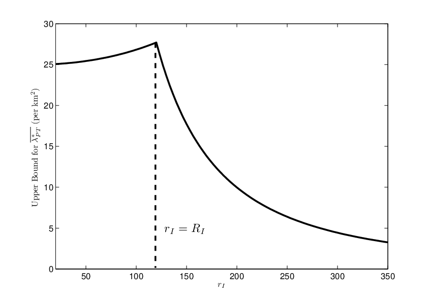
Let $r_{I}$ and $R_{I}$ denote the interference range of the secondary and the primary users, respectively. For a fixed $R_{I}$ , the upper bound on $\overline{\lambda^{*}_{PT}}$ given in T2.2 is maximized when the primary and secondary networks have matching interference ranges: $r_{I}=R_{I}$ .

Proof:

Since under the disk signal propagation and interference model, $r_{p}=\beta r_{I}$ for some $\beta\in(0,1)$ , the upper bound on $\overline{\lambda^{*}_{PT}}$ can be written as

\displaystyle\overline{\lambda^{*}_{PT}}\leq\left\{\begin{array}[]{ll}\frac{\lambda_{c}(1)}{4R_{I}^{2}-\beta^{2}r_{I}^{2}}&\textrm{ for $r_{I}\leq R_{I}$,}\\ \frac{\lambda_{c}(1)}{(4-\beta^{2})r_{I}^{2}}&\textrm{ for $r_{I}>R_{I}$.}\end{array}\right.

Then the above theorem can be readily shown by finding the maximal point for the two cases: $r_{I}\leq R_{I}$ and $r_{I}>R_{I}$ . ∎

An example of the upper bound on $\overline{\lambda^{*}_{PT}}$ is plotted as a function of $r_{I}$ in Fig. 10. Notice that there is a distinct difference in the slope on the two sides of the optimal point. As a consequence, the operating region of $r_{I}<R_{I}$ is preferred over that of $r_{I}>R_{I}$ when the optimal point $r_{I}=R_{I}$ cannot be achieved. We point out that the desired operating region of $r_{I}<R_{I}$ is the typical case of a secondary network coexisting with a privileged primary network.

V Proofs

In this section, we present proofs of the main results presented in Sec. III-IV. We start with a brief overview of several basic results in percolation and ergodic theory that will be used in the proofs.

V-A Percolation and Ergodic Theory

V-A1 Poisson Boolean Model

Poisson Boolean model is a common model in continuum percolation [13]. Often referred to as $\mathcal{B}(X,~\rho,~\lambda)$ , the model is specified by two elements: a Poisson point process $X$ on $\mathbb{R}^{d}$ with density $\lambda$ and a radius random variable $\rho$ with a given distribution. Under this model, each point in $X$ is the center of a circle in $\mathbb{R}^{d}$ with a random radius distributed according to the distribution of $\rho$ . Radii associated with different points are independent, and they are also independent of points in $X$ . Under a Poisson Boolean model, the whole space is partitioned into two regions: the occupied region, which is the region covered by at least one ball, and the vacant region, which is the complement of the occupied region. We define occupied (vacant) components as those connected components in the occupied (vacant) region.

Assume that nodes in a homogeneous ad hoc network form a Poisson point process with density $\lambda$ and their transmission range is $r$ . It is easy to see that the connectivity of this network can be studied through examining the occupied connected components in the corresponding Poisson Boolean model $\mathcal{B}(X,~r/2,~\lambda)$ .

V-A2 Sharp Transition in Two Dimensions

Phase transition is a well-known phenomenon in percolation. For the Poisson Boolean model in two dimensions, this phenomenon appears more remarkable in the sense that the critical density for the a.s. existence of infinite occupied components is equal to that for the a.s. existence of infinite vacant components. Let $\lambda_{c}(2\rho)$ denote the critical density for the Poisson Boolean model $\mathcal{B}(X,~\rho,~\lambda)$ , then we have that

$\Box$

when $\lambda<\lambda_{c}(2\rho)$ , there is no infinite occupied component a.s. and there is a unique infinite vacant component a.s.;
$\Box$

when $\lambda>\lambda_{c}(2\rho)$ , there is a unique infinite occupied component a.s. and there is no infinite vacant component a.s.

The exact value of $\lambda_{c}$ is not known. For a deterministic radius $\rho$ , simulation results [19] indicate that $\lambda_{c}(2\rho)\approx 0.36\rho^{-2}$ , while rigorous bounds $0.192\rho^{-2}<\lambda_{c}(2\rho)<0.843\rho^{-2}$ are provided in [13, 20].

V-A3 Crossing Probabilities

A continuous curve in the occupied region is called an occupied path. An occupied path $\gamma$ is an occupied L-R crossing of the rectangle $\{0\leq x\leq l_{1}\}\times\{0\leq y\leq l_{2}\}$ if $\gamma$ intersects with both the left and the right boundaries of the rectangle, i.e., $\gamma\cap(\{x=0\}\times\{0\leq y\leq l_{2}\})\neq\phi$ , $\gamma\cap(\{x=l_{1}\}\times\{0\leq y\leq l_{2}\})\neq\phi$ , and the segment between the two intersecting points is fully contained in the rectangle (see Fig. 11(a)). Similarly, we define an occupied T-B crossing by requiring that $\gamma$ intersects with the top and bottom boundaries of the rectangle (see Fig. 11(b)). Let

	$\displaystyle\sigma((l_{1},l_{2}),~\lambda,~\textrm{L-R})$	$\displaystyle=$	$\displaystyle\textrm{Pr}\{\exists\textrm{ an occupied L-R crossing of $[0,l_{1}]\times[0,l_{2}]$}\},$
	$\displaystyle\sigma((l_{1},l_{2}),~\lambda,~\textrm{T-B})$	$\displaystyle=$	$\displaystyle\textrm{Pr}\{\exists\textrm{ an occupied T-B crossing of $[0,l_{1}]\times[0,l_{2}]$}\},$

denote the two crossing probabilities in the rectangle $[0,l_{1}]\times[0,l_{2}]$ . Then for a Poisson Boolean model $\mathcal{B}(X,~\rho,~\lambda)$ in two dimensions with a.s. bounded $\rho$ , we have [13, Corollary 4.1] that for any $k\geq 1$ ,

\underset{n\rightarrow\infty}{\lim}\sigma((kn,n),~\lambda,~\textrm{L-R})=\left\{\begin{array}[]{ll}1,&\textrm{ if }\lambda>\lambda_{c}(2\rho);\\ 0,&\textrm{ if }\lambda<\lambda_{c}(2\rho).\end{array}\right.

(6)

Due to the symmetry of the Poisson Boolean model, similar results hold for the T-B crossing probability $\sigma((n,kn),~\lambda,~\textrm{T-B})$ .

V-A4 Dependent Edge-Percolation Model

Let $\mathcal{L}$ be a square lattice on $\mathbb{R}^{2}$ with side length $d$ (see Fig. 12). In an edge-percolation model, every site in $\mathcal{L}$ is occupied but every edge in $\mathcal{L}$ exists with some probability $p$ . An existing edge is often referred to as an open edge, and an edge that is not open is called closed. When the states (open/closed) of edges are correlated, we have a dependent edge percolation model.

Consider a special case of dependent edge-percolation model $\mathcal{L}$ where the state of an edge $e$ is only correlated with its six adjacent edges (edges that share a common point with $e$ ). We have the following known result.

Fact 1

[4, Proposition 1]
For any collection $\{e_{i}\}_{i=1}^{n}$ of $n$ distinct edges in $\mathcal{L}$ , we have

\displaystyle\textrm{Pr}\{(C_{1}=0)\cap(C_{2}=0)\cap\cdots\cap(C_{n}=0)\}\leq q^{\frac{n}{4}},

where $C_{i}$ is the indicator of $e_{i}$ being open,, and $q=1-p$ is the probability of an edge being closed.

V-A5 Ergodic Theory

The study object of ergodic theory is the so-called measure-preserving (m.p.) dynamical system $(\Omega,~\mathscr{F},~\mu,~T)$ , which consists of a set $\Omega$ , a $\sigma$ -algebra $\mathscr{F}$ of measurable subsets of $\Omega$ , a nonnegative measure $\mu$ on $(\Omega,~\mathscr{F})$ , and an invertible m.p. transformation $T:~\Omega\rightarrow\Omega$ such that $\mu(T^{-1}F)=\mu(F)$ for all $F\in\mathscr{F}$ . A set $F\in\mathscr{F}$ is said to be T-invariant if $T^{-1}F=F$ . Obviously, all T-invariant sets in $\mathscr{F}$ form a $\sigma$ -algebra.

An m.p. dynamical system $(\Omega,~\mathscr{F},~\mu,~T)$ is said to be ergodic if the $\sigma$ -algebra of T-invariant sets is trivial, i.e., for any invariant set, either it has measure zero or its complement has measure zero. Another property of the m.p. dynamical system that implies ergodicity is called mixing: an m.p. dynamical system $(\Omega,~\mathscr{F},~\mu,~T)$ is said to be mixing if for all $E,F\in\mathscr{F}$ , $\mu(T^{n}E\cap F)-\mu(E)\mu(F)\rightarrow 0$ as $n\rightarrow\infty$ . For a m.p. dynamical system which is a product of two m.p. dynamical systems, we have the following classical result in ergodic theory.

Fact 2

[22, Theorem 2.6.1]
The product system of a mixing m.p. dynamical system and an ergodic m.p. dynamic system is ergodic, that is, for a mixing $(\Omega,~\mathscr{F},~\mu,~T)$ and an ergodic $(\Psi,~\mathscr{L},~\nu,~S)$ , the product system $(\Omega\times\Psi,~\mathscr{F}\times\mathscr{L},~\mu\times\nu,~T\times S)$ is ergodic, where $\mathscr{F}\times\mathscr{L}$ is the $\sigma$ -algebra on $\Omega\times\Psi$ generated by subsets of the form $F\times L$ $(F\in\mathscr{F},L\in\mathscr{L})$ and $\mu\times\nu$ is the corresponding product measure.

The concepts of ergodicity and mixing can also be defined for a random model under a probability space $(\Omega,\mathscr{F},\mu)$ , where the m.p. transformation $T$ is replaced by a transformation group $\{S_{x}:~x\in\mathbb{R}^{d}\textrm{ or }\mathbb{Z}^{d}\}$ indexed by $\mathbb{R}^{d}$ or $\mathbb{Z}^{d}$ . For a point process model, the transformation $S_{x}$ is usually to shift the realization $\omega\in\Omega$ by $x$ . A random model under a probability space $(\Omega,\mathscr{F},\mu)$ is said to be ergodic if there exists a transformation group $\{S_{x}:~x\in\mathbb{R}^{d}\textrm{ or }\mathbb{Z}^{d}\}$ that acts ergodically on $(\Omega,\mathscr{F},\mu)$ . A transformation group $\{S_{x}:~x\in\mathbb{R}^{d}\textrm{ or }\mathbb{Z}^{d}\}$ is said to act ergodically if the $\sigma$ -algebra of events invariant under the whole group is trivial, i.e., any invariant event has measure either zero or one. Moreover, a random model under a probability space $(\Omega,\mathscr{F},\mu)$ is said to be mixing if there exists a transformation group $\{S_{x}:~x\in\mathbb{R}^{d}\textrm{ or }\mathbb{Z}^{d}\}$ such that for all $E,F\in\mathscr{F}$ , we have $\mu(S_{x}E\cap F)-\mu(E)\mu(F)\rightarrow 0$ as $|x|\rightarrow\infty$ . One direct consequence of an ergodic random model is presented as below.

Fact 3

For an ergodic random model $(\Omega,\mathscr{F},\mu)$ , if an event $E\in\mathscr{F}$ invariant under the whole transformation group $\{S_{x}:~x\in\mathbb{R}^{d}\textrm{ or }\mathbb{Z}^{d}\}$ occurs wpp., i.e., $\mu(E)>0$ , then it occurs a.s., i.e., $\mu(E)=1$ .

V-B Proof of Theorem 1

V-B1 Proof of T1.1

To prove T1.1, it suffices to show that for any two given points $(\lambda_{S1},\lambda_{PT1})$ and $(\lambda_{S2},\lambda_{PT2})$ in ${\cal C}$ , we can find a path in ${\cal C}$ that connects these two points. In particular, the path we constructed is given by a horizontal segment and a vertical segment as shown in Fig. 13, where we assume, without loss of generality, that $\lambda_{S1}\leq\lambda_{S2}$ .

Consider case (a) in Fig. 13 where $\lambda_{PT1}\leq\lambda_{PT2}$ . Case (b) can be proven similarly. First we show every point $(\lambda_{S},\lambda_{PT1})$ $(\lambda_{S1}\leq\lambda_{S}\leq\lambda_{S2})$ on the horizontal segment belongs to ${\cal C}$ . Let $\lambda^{\prime}=\lambda_{S}-\lambda_{S1}$ . A Poisson point process $X$ with density $\lambda_{S}$ is statistically equivalent to the superposition of a Poisson point process $X_{1}$ with density $\lambda_{S1}$ and an independent Poisson point process $X^{\prime}$ with density $\lambda^{\prime}$ . It follows that any realization of the heterogeneous network with densities $\lambda_{S}$ and $\lambda_{PT1}$ can be generated by adding more secondary nodes to a realization of the heterogeneous network with densities $\lambda_{S1}$ and $\lambda_{PT1}$ . Thus, the existence of an infinite connected component in ${\cal G}(\lambda_{S1},\lambda_{PT1})$ implies the existence of an infinite connected component in ${\cal G}(\lambda_{S},\lambda_{PT1})$ . We thus have that $(\lambda_{S},\lambda_{PT1})\in{\cal C}$ for $(\lambda_{S1}\leq\lambda_{S}\leq\lambda_{S2})$ .

Now we know that the two end points $(\lambda_{S2},\lambda_{PT1})$ and $(\lambda_{S2},\lambda_{PT2})$ of the vertical segment belong to ${\cal C}$ . For a point $(\lambda_{S2},\lambda_{PT})$ $(\lambda_{PT1}\leq\lambda_{PT}\leq\lambda_{PT2})$ on the vertical segment, let $\lambda^{\prime}=\lambda_{PT2}-\lambda_{PT}$ , then any realization of the heterogeneous network with densities $\lambda_{S2}$ and $\lambda_{PT}$ can be obtained by independently removing each primary transmitter-receiver pair with probability $\lambda^{\prime}/\lambda_{PT2}$ from a realization of the heterogeneous network with densities $\lambda_{S2}$ and $\lambda_{PT2}$ . It follows from the definition of communication link in the secondary network (see Sec. II-B1) that the existence of an infinite connected component in ${\cal G}(\lambda_{S2},\lambda_{PT2})$ implies the existence of an infinite connected component in ${\cal G}(\lambda_{S},\lambda_{PT})$ . Thus, we have $(\lambda_{S2},\lambda_{PT})\in{\cal C}$ $(\lambda_{PT1}\leq\lambda_{PT}\leq\lambda_{PT2})$ .

V-B2 Proof of Theorem 1.2

Suppose that $(\lambda_{S},\lambda_{PT})\in{\cal C}$ $(\lambda_{PT}>0)$ , then by using the coupling argument for showing that the vertical segment belongs to ${\cal C}$ in the above proof of T1.1, we conclude that $(\lambda_{S},0)\in{\cal C}$ , i.e., the $\lambda_{S}$ -axis is the lower boundary of ${\cal C}$ .

Suppose that $\lambda_{S2}>\lambda_{S1}>0$ . In order to prove the monotonicity of $\lambda^{*}_{PT}(\lambda_{S})$ with $\lambda_{S}$ it suffices to show that $\forall~\lambda_{PT}\geq 0$ , if $(\lambda_{S1},\lambda_{PT})\in{\cal C}$ then $(\lambda_{S2},\lambda_{PT})\in{\cal C}$ . This is a direct consequence of the coupling argument for showing that the horizontal segment belongs to ${\cal C}$ in the above proof of T1.1.

V-B3 Proof of Theorem 1.3

We first establish the ergodicity of the heterogeneous network model.

Lemma 1

The heterogeneous network model is ergodic.

Proof:

The proof of this lemma is inspired by the proof of the ergodicity of Poisson Boolean model [13, Proposition 2.8]. The difficulty here is that for the heterogeneous network model, we have two correlated Poisson point processes: the primary transmitters and the primary receivers. The definition of the shift transformation for the primary network model is thus more complicated than the standard Poisson Boolean model with a deterministic radius $\rho$ . To prove Lemma 1, we first show the ergodicity of the primary network model, and then we show the mixing property of the secondary network model. Since the primary network model is independent of the secondary network model, it follows from Fact 2 that the heterogeneous network model is ergodic.

Let $\mathscr{B}^{d}$ denote the Borel $\sigma$ -algebra in $\mathbb{R}^{d}$ , and $N$ the set of all simple counting measures⁶⁶ 6 A simple counting measure on $\mathscr{B}^{d}$ is an integer-valued measure for which the measures of bounded Borel sets are all finite and the measure of a point is at most 1. on $\mathscr{B}^{d}$ . Construct a $\sigma$ -algebra $\mathscr{N}$ for $N$ generated by sets of the form

\displaystyle\{n\in N:~n(A)=k\},

where $A\in\mathscr{B}^{d}$ and $k$ is an integer. A point process $X$ can now be defined as a measurable mapping from a probability space $(\Omega,~\mathscr{F},~P)$ into $(N,~\mathscr{N})$ [21, Chapter 7]. The measure $\mu$ on $\mathscr{N}$ induced by $X$ is defined as $\mu(G)=P(X^{-1}(G))$ , for all $G\in\mathscr{N}$ .

In order to define the shift transformation on $\Omega$ , it is convenient to identify $(\Omega,~\mathscr{F})$ with $(N,~\mathscr{N})$ . Let $\omega(A)$ denote the number of points in $A\in\mathscr{B}^{d}$ , $\forall~\omega\in\Omega$ , and $T_{x}$ be the shift according to a vector $x\in\mathbb{R}^{d}$ . Then $T_{x}$ induces a shift transformation $S_{x}:~\Omega\rightarrow\Omega$ through the equation for every $A\in\mathscr{B}^{d}$ ,

\displaystyle(S_{x}\omega)(A)=\omega(T_{x}^{-1}A).

(7)

Let $(\Omega_{PT},~\mathscr{F}_{PT},~P_{PT})$ be the probability space of the Poisson point process $X_{PT}$ for the primary transmitters with density $\lambda_{PT}$ . Let $\Omega_{PR}$ be the product space $\prod_{n\in\mathbb{N}}\prod_{z\in\mathbb{Z}^{2}}C_{R_{p}}$ for the primary receivers, where $C_{R_{p}}=\{(x,y):~x^{2}+y^{2}\leq R_{p}\}$ . Then we equip $\Omega_{PR}$ with the usual product $\sigma$ -algebra and product measure $P_{PR}$ with all marginal probability measure being $\mu_{U}$ , where $\mu_{U}$ is a uniform probability measure on $C_{R_{p}}$ . Finally, we set $\Omega_{P}=\Omega_{PT}\times\Omega_{PR}$ and equip $\Omega_{P}$ with the product measure $P_{P}=P_{PT}\times P_{PR}$ and the usual product $\sigma$ -algebra. It follows that the primary network model is a measurable mapping from $\Omega_{P}$ into $N_{PT}\times\Omega_{PR}$ defined by $(\omega_{PT},~\omega_{PR})\rightarrow(X_{PT}(\omega_{PT}),~\omega_{PR})$ , where $N_{PT}$ is specified in the definition of the point process.

The positions of the primary transmitters corresponding to $(\omega_{PT},~\omega_{PR})\in\Omega_{PT}\times\Omega_{PR}$ are easily known from $\omega_{PT}$ . For the primary receivers, the positions are obtained as follows. Consider binary cubes

\displaystyle K(n,z):=\prod_{i=1}^{2}(z_{i}2^{-n},(z_{i}+1)2^{-n}]~~\textrm{ for all }n\in\mathbb{N}\textrm{ and }z\in\mathbb{Z}^{2}.

For each primary transmitter $x_{PT}$ , there exists a unique smallest integer $n_{0}=n_{0}(x_{PT})$ such that it is contained in a binary cube $K(n_{0},z(n_{0},x_{PT}))$ which contains no other primary transmitters. The relative position of $x_{PT}$ ’s receiver with respect to $x_{PT}$ is then given by $\omega_{PR}(n_{0},z(n_{0},x_{PT}))$ .

Let $e_{1}$ , $e_{2}$ denote the unit vectors in $\mathbb{R}^{2}$ , then the translation $T_{e_{i}}:~\mathbb{R}^{2}\rightarrow\mathbb{R}^{2}$ $(i=1,2)$ defined by $x\rightarrow x+e_{i}$ induces a shift transformation $U_{e_{i}}$ on $\Omega_{PR}$ through the equation

\displaystyle(U_{e_{i}}\omega_{PR})(n,z)=\omega_{PR}(n,z-2^{n}e_{i}),\textrm{ for $i=1,2$}.

Hence $T_{e_{i}}$ also induces a shift transformation $\tilde{T}_{e_{i}}$ on $\Omega_{P}=\Omega_{PT}\times\Omega_{PR}$ as follows:

\displaystyle\tilde{T}_{e_{i}}(\omega_{P})=(S_{e_{i}}\omega_{PT},~U_{e_{i}}\omega_{PR}),\textrm{ for $i=1,2$},

where $S_{e_{i}}$ is defined in (7). By using techniques similar to the proof of Boolean models [13, Proposition 2.8], we have that the m.p. dynamical system $(\Omega_{P},~\mathscr{F}_{P},~P_{P},~\tilde{T}_{e_{1}})$ is ergodic.

Since the transmission range $r_{p}$ of secondary users is fixed, the probability space of the secondary network model is the probability space $(\Omega_{S},~\mathscr{F}_{S},~P_{S})$ for the Poisson point process $X_{S}$ of secondary users with density $\lambda_{S}$ . It follows from the proof of Poisson point processes [13, Proposition 2.6] that the m.p. dynamical system $(\Omega_{S},~\mathscr{F}_{S},~P_{S},~S_{e_{1}})$ is mixing.

Since the primary network model is independent of the secondary network model, the sample space of the heterogeneous network model $\Omega$ can be written as the product of $\Omega_{P}$ and $\Omega_{S}$ , ${\it i.e.,\ \/}$ $\Omega=\Omega_{P}\times\Omega_{S}$ . We equip $\Omega$ with product measure $P=P_{P}\times P_{S}$ and the usual product $\sigma$ -algebra. Similarly, the translation $T_{e_{i}}$ ( $i=1,2$ ) induces a transformation $\hat{T}_{e_{i}}$ on $\Omega=\Omega_{P}\times\Omega_{S}$ , which is given by

\displaystyle\hat{T}_{e_{i}}(\omega)=(\tilde{T}_{e_{i}}\omega_{P},S_{e_{i}}\omega_{S}).

Then it follows from Fact 2 that the product m.p. dynamical system $(\Omega,~\mathscr{F},~P,~\hat{T}_{e_{1}})$ is ergodic. Since the $\sigma$ -algebra invariant under the transformation group $\{\hat{T}_{z}:~z\in\mathbb{Z}^{2}\}$ is a subset of the $\sigma$ -algebra invariant under the transformation $\hat{T}_{e_{1}}$ , we conclude that $\{\hat{T}_{z}:~z\in\mathbb{Z}^{2}\}$ acts ergodically, i.e., the heterogeneous network model is ergodic. ∎

Based on Lemma 1, we have the following lemma.

Lemma 2

The number of infinite connected component in ${\cal G}(\lambda_{S},\lambda_{PT})$ is a constant a.s., and it can only take value from $\{0,~1,~\infty\}$ .

Proof:

Let $K$ denote the (random) number of infinite connected components in $\mathcal{G}(\lambda_{S},\lambda_{PT})$ , then since for all $k\geq 0$ , the event $\{K=k\}$ is invariant under the group of shift transformations, it follows from Lemma 1 and Fact 3 that the event occurs with probability $0$ or $1$ . Consequently, we have that $K$ is an a.s. constant. Then it suffices to exclude the possibility of $K\geq 2$ . This is shown by contradiction, that is, if there exist $K\geq 2$ infinite connected components, then they can be linked together as one connected component wpp. The proof is inspired by the proof of Proposition 3.3 in [13], and a major difference is that here we need to consider the impact of the primary network on the connectivity of the secondary network.

Suppose that there are $K\geq 2$ infinite connected components a.s. If we remove all the secondary nodes centered inside a box $B=[-n,n]^{2}$ , then the resulting secondary network should contain at least $K$ unbounded components a.s. Let, for $A\subseteq\mathbb{R}^{2}$ , $\mathcal{G}[A]$ denote the graph formed by secondary nodes in $A$ . Given a box $B$ and $\epsilon>0$ , consider the event

\displaystyle E(B,\epsilon):=\left\{\textrm{$d(U,B)\leq r_{p}-\epsilon$ for any infinite connected component $U$ in $\mathcal{G}[B^{c}]$}\right\}.

Partition the box $B$ into squares with side length $a>0$ and let $\mathcal{S}_{a}=\{S_{1},...,S_{N}\}$ denote the collection of all the squares which are adjacent to the boundary of $B$ . Clearly, for a box $B$ and $\epsilon>0$ , we can find $a=a(B,\epsilon)\in(0,r_{p}/\sqrt{5})$ and $\eta=\eta(a)>0$ such that for any point $x\notin B$ with $d(x,B)\leq r_{p}-\epsilon/2$ , there exists a square $S=S(x)\in\mathcal{S}_{a}$ for which we have $\sup_{y\in S}d(x,y)\leq r_{p}-\eta$ . This means that, if we center in each square of $\mathcal{S}_{a}$ a secondary node and there are neither primary transmitters nor primary receivers within a bigger box $\bar{B}=[-n-\max\{r_{I},R_{I}\},n+\max\{r_{I},R_{I}\}]^{2}$ , then every infinite component $U$ in $\mathcal{G}[B^{c}]$ with $d(U,B)\leq r_{p}-\epsilon$ is connected to some secondary node in $\mathcal{S}_{a}$ .

Let $E(a,\eta)$ be the event that each square in $\mathcal{S}_{a}$ contains at least one secondary node and $E(\bar{B})$ the event that there are neither primary transmitters nor primary receivers within $\bar{B}$ . Since $E(a,\eta)$ depends on the configuration of secondary nodes inside the box $B$ , $E(B,\epsilon)$ depends on the configuration of secondary nodes outside $B$ and the configuration of primary nodes, based on the independence of the primary network and the secondary network, we have

\displaystyle\textrm{Pr}(E(B,\epsilon)\cap E(a,\eta)\cap E(\bar{B}))=\textrm{Pr}(E(B,\epsilon))\textrm{Pr}(E(a,\eta))\textrm{Pr}(E(\bar{B})|E(B,\epsilon)).

If $E(B,\epsilon)$ , $E(a,\eta)$ and $E(\bar{B})$ all occur wpp., then there is only one infinite connected component⁷⁷ 7 Since $a<r_{p}/\sqrt{5}$ , every secondary node in a square of $\mathcal{S}_{a}$ is connected to those secondary nodes in the neighboring squares. wpp. By using arguments similar to the proof for Proposition 3.3 in [13], we have that there exists a large enough box $B$ and $\epsilon>0$ such that $\textrm{Pr}(E(B,\epsilon))>0$ . Obviously, $\textrm{Pr}(E(a,\eta))>0$ . Moreover, it is easy to see that $P(E(\bar{B})|E(B,\epsilon))\geq P(E(\bar{B}))>0$ . ∎

Now we have that the number $K$ of infinite connected components is equal to zero, one or infinity a.s. To exclude the possibility of $K=\infty$ , we can directly apply the proof of Poisson Boolean models [13, Theorem 3.6] here, which is based on several combinatorial results. The details are omitted.

V-C Proof of Theorem 2

V-C1 Proof of T2.1

To prove T2.1, it suffices to show that

(a)

for any $\lambda_{S}\leq\lambda_{c}(r_{p})$ , the secondary network is not connected for any $\lambda_{PT}\geq 0$ ;
(b)

for any $\lambda_{S}>\lambda_{c}(r_{p})$ , there exists a $\lambda^{*}_{PT}(\lambda_{S})>0$ such that $\forall~\lambda_{PT}\leq\lambda^{*}_{PT}(\lambda_{S})$ , the secondary network is connected.

From Sec. V-A, we know that for a Poisson homogeneous ad hoc network with density $\lambda$ and transmission range $r$ , the necessary and sufficient condition for connectivity is $\lambda>\lambda_{c}(r)$ . Since the existence of an infinite connected component in the secondary network implies the existence of an infinite connected component in the homogeneous ad hoc network with the same density and the same transmission range, by using a coupling argument, we conclude that when $\lambda_{S}\leq\lambda_{c}(r_{p})$ , there does not exist an infinite connected component a.s. in the secondary network for any $\lambda_{PT}\geq 0$ . This proves part (a).

The basic idea of the proof of part (b) is to approximate the secondary network $\mathcal{G}(\lambda_{S},\lambda_{PT})$ by a discrete dependent edge-percolation model on the grid. This discrete dependent edge-percolation model $\mathcal{L}$ is constructed in a way such that the existence of an infinite connected component in $\mathcal{L}$ implies the existence of an infinite connected component in $\mathcal{G}(\lambda_{S},\lambda_{PT})$ .

Construct the square lattice $\mathcal{L}$ on $\mathbb{R}^{2}$ with side length $d$ (see Fig. 12). Note that each site in $\mathcal{L}$ is virtual and is not related to any node either in the secondary network or in the primary network. Next we specify the conditions for an edge being open in $\mathcal{L}$ , which is the key to the mapping from $\mathcal{G}(\lambda_{S},\lambda_{PT})$ to $\mathcal{L}$ .

For each edge $e$ in $\mathcal{L}$ , let $(x_{e},~y_{e})$ denote the middle point of $e$ . Then we introduce three random fields $A_{e}$ , $B_{e}$ , and $C_{e}$ , all associated with the edge $e$ in $\mathcal{L}$ , where $C_{e}=A_{e}B_{e}$ is the indicator of the edge $e$ being open, $A_{e}$ represents the condition (C1) of the distance between two users for the existence of a communication link in the secondary network, and $B_{e}$ represents the condition (C2) of the spectrum opportunity. Specifically, consider the Poisson Boolean model $\mathcal{B}(X_{S},~r_{p}/2,~\lambda_{S})$ where $X_{S}$ is the Poisson point process generated by secondary users, then for a horizontal edge $e$ , $A_{e}=1$ if the following two events (illustrated in Fig. 14) are true:

(i)

there is an occupied L-R crossing of the rectangle $[x_{e}-3d/4,~x_{e}+3d/4]\times[y_{e}-d/4,~y_{e}+d/4]$ in $\mathcal{B}(X_{S},~r_{p}/2,~\lambda_{S})$ ;
(ii)

there are two occupied T-B crossings of the square $[x_{e}-3d/4,~x_{e}-d/4]\times[y_{e}-d/4,~y_{e}+d/4]$ and the square $[x_{e}+d/4,~x_{e}+3d/4]\times[y_{e}-d/4,~y_{e}+d/4]$ in $\mathcal{B}(X_{S},~r_{p}/2,~\lambda_{S})$ ;

and $A_{e}=0$ otherwise. For a vertical edge $e$ , the definition of $A_{e}$ is similar, where the horizontal and vertical coordinates are switched in the above two events.

Next we define the random field $B_{e}$ . For an edge $e$ in $\mathcal{L}$ , $B_{e}=1$ if $A_{e}=1$ and the following two events are true:

(i)

there is no primary transmitter within distance $R_{I}$ of any secondary node of the three crossings in the definition of $A_{e}$ ;
(ii)

there is no primary receiver within distance $r_{I}$ of any secondary node of the three crossings in the definition of $A_{e}$ ;

and $B_{e}=0$ otherwise. It follows from the definition of communication link in the secondary network (see Sec. II-B1) that if $A_{e}=1$ and $B_{e}=1$ , then the three crossings in $\mathcal{B}(X_{S},~r_{p}/2,~\lambda_{S})$ are also three crossings in $\mathcal{G}(\lambda_{S},\lambda_{PT})$ .

Let $C_{e}=A_{e}B_{e}$ , then we claim that the edge $e$ is open if $C_{e}=1$ , and $e$ is closed if $C_{e}=0$ . We observe from Fig. 14 that whether the edge $e$ is open is correlated with the states of the other edges. This model $\mathcal{L}$ thus is a dependent edge-percolation model. Furthermore, as shown in Fig. 15, if there exists an infinite open connected component in $\mathcal{L}$ , then those crossings associated with the edges in the infinite component in $\mathcal{L}$ comprise an infinite connected component in $\mathcal{G}(\lambda_{S},\lambda_{PT})$ . As a consequence, by considering the uniqueness of the infinite connected component in $\mathcal{G}(\lambda_{S},\lambda_{PT})$ , we only need to prove the following lemma in order to show T2.1.

Lemma 3

Let $C(O)$ denote the open connected component containing the origin $O$ in $\mathcal{L}$ . Then given $\lambda_{S}>\lambda_{c}(r_{p})$ , $\exists~D>0$ , $\lambda^{*}_{PT}>0$ such that for $d=D$ and any $\lambda_{PT}\leq\lambda^{*}_{PT}$ , we have

\displaystyle\textrm{Pr}\{|C(O)|=\infty\}>0,

where $|C(O)|$ is the number of edges in $C(O)$ .

Proof:

For an arbitrary edge $e$ in $\mathcal{L}$ , let $q=\textrm{Pr}\{C_{e}=0\}$ , then we have

\displaystyle q=\textrm{Pr}\{(A_{e}=0)\cup(B_{e}=0)\}\leq\textrm{Pr}\{A_{e}=0\}+\textrm{Pr}\{B_{e}=0\}.

From the result on the crossing probabilities given in (6), we know that when $\lambda_{S}>\lambda_{c}(r_{p})$ ,

$\displaystyle\textrm{Pr}\{A_{e}=0\}$	$\displaystyle=$	$\displaystyle\textrm{Pr}\{\textrm{at least one crossing does not exist}\}$
	$\displaystyle\leq$	$\displaystyle\left[1-\sigma\left(\left(\frac{3d}{2},\frac{d}{2}\right),~\lambda_{S},~\textrm{L-R}\right)\right]+\left[1-\sigma\left(\left(\frac{d}{2},\frac{d}{2}\right),~\lambda_{S},~\textrm{T-B}\right)\right]$
		$\displaystyle+\left[1-\sigma\left(\left(\frac{d}{2},\frac{d}{2}\right),~\lambda_{S},~\textrm{T-B}\right)\right]$
	$\displaystyle\rightarrow$	$\displaystyle 0~~~~\textrm{as}~~~~d\rightarrow\infty,~~~~{\it i.e.,\ \/}\underset{d\rightarrow\infty}{\lim}\textrm{Pr}\{A_{e}=0\}=0.$

Thus when $\lambda_{S}>\lambda_{c}(r_{p})$ , $\forall\epsilon>0$ , $\exists~D>0$ such that $\textrm{Pr}\{A_{e}=0\}<\frac{\epsilon}{3}$ .

Given $A_{e}=1$ , let $S_{R_{I}}$ be the area of the region covered by the circles with radii $R_{I}$ centered at those secondary nodes in the three crossings, and $S_{r_{I}}$ be the area of the region covered by the circles with radii $r_{I}$ centered at those secondary nodes in the three crossings. Then we have

	$\displaystyle\textrm{Pr}\{B_{e}=0~\|~A_{e}=1\}$	$\displaystyle=$	$\displaystyle\textrm{Pr}\{\exists~\textrm{some primary transmitter in $S_{R_{I}}$}\}$
			$\displaystyle+\textrm{Pr}\{\exists~\textrm{some primary receiver in $S_{r_{I}}$}\}.$

Since $S_{R_{I}}\leq\left(\frac{3d}{2}+2R_{I}+r_{p}\right)\left(\frac{d}{2}+2R_{I}+r_{p}\right)$ and $S_{r_{I}}\leq\left(\frac{3d}{2}+2r_{I}+r_{p}\right)\left(\frac{d}{2}+2r_{I}+r_{p}\right)$ , it follows from the basic property of Poisson point processes that

	$\displaystyle\textrm{Pr}\{B_{e}=0~\|~A_{e}=1\}$	$\displaystyle\leq$	$\displaystyle 1-\exp\left[-\lambda_{PT}\left(\frac{3d}{2}+2R_{I}+r_{p}\right)\left(\frac{d}{2}+2R_{I}+r_{p}\right)\right]$
			$\displaystyle+1-\exp\left[-\lambda_{PT}\left(\frac{3d}{2}+2r_{I}+r_{p}\right)\left(\frac{d}{2}+2r_{I}+r_{p}\right)\right].$

Obviously, $\underset{\lambda_{PT}\rightarrow 0}{\lim}~\textrm{Pr}\{B_{e}=0~|~A_{e}=1\}=0$ for fixed $d$ . Thus if we choose $d=D$ , then $\forall\epsilon>0$ , $\exists~\lambda^{*}_{PT}>0$ such that

\displaystyle\textrm{Pr}\{B_{e}=0~|~A_{e}=1\}<\frac{\epsilon}{3}~~\textrm{for all $\lambda_{PT}\leq\lambda^{*}_{PT}$.}

It implies that when $d=D$ , for all $\lambda_{PT}\leq\lambda^{*}_{PT}$ ,

$\displaystyle\textrm{Pr}\{B_{e}=0\}$	$\displaystyle=$	$\displaystyle\textrm{Pr}\{A_{e}=0\}+\textrm{Pr}\{B_{e}=0~\|~A_{e}=1\}\textrm{Pr}\{A_{e}=1\}$
	$\displaystyle\leq$	$\displaystyle\textrm{Pr}\{A_{e}=0\}+\textrm{Pr}\{B_{e}=0~\|~A_{e}=1\}$
	$\displaystyle<$	$\displaystyle\frac{2\epsilon}{3}.$

Thus for $d=D$ and all $\lambda_{PT}\leq\lambda^{*}_{PT}$ , we have

q\leq\textrm{Pr}\{A_{e}=0\}+\textrm{Pr}\{B_{e}=0\}<\epsilon.

(8)

From Fig. 14, we can see that if $d\geq\max\{4R_{I}+2r_{p},~4r_{I}+2r_{p}\}$ , then the state of edge $e$ is only correlated with its six adjacent edges and it is independent of other edges. In this case, by using the ‘Peierls argument⁸⁸ 8 The essence of ‘Peierls argument’ is to make use of the one-to-one correspondence between a finite open component in lattice $\mathcal{L}$ containing the origin $O$ and a closed circuit in the dual lattice $\mathcal{L}^{+}$ of $\mathcal{L}$ surrounding the origin $O$ .’ [23, Chapter 1], we can show that if the probability of an edge being closed $q<\left(\frac{11-2\sqrt{10}}{27}\right)^{4}$ , then

\displaystyle\textrm{Pr}\{|C(O)|=\infty\}>0.

(9)

The proof of the above statement follows the proof of Theorem 3 in [3] except that the upper bound on the probability of $n$ edges all being closed is replaced by the one given in Fact 1.

Thus by combining (9) with (8), we conclude that given $\lambda_{S}>\lambda_{c}(r_{p})$ , $\exists~D>0$ , $\lambda^{*}_{PT}>0$ such that for fixed $d=\max\{D,4R_{I}+2r_{p},~4r_{I}+2r_{p}\}$ and any $\lambda_{PT}\leq\lambda^{*}_{PT}$ ,

\displaystyle\textrm{Pr}\{|C(O)|=\infty\}>0.

Notice that $\lambda^{*}_{PT}$ depends on $D$ which is chosen according to the crossing probability and is determined by $\lambda_{S}$ . As a consequence, $\lambda^{*}_{PT}$ is a function of $\lambda_{S}$ , ${\it i.e.,\ \/}$ $\lambda^{*}_{PT}=\lambda^{*}_{PT}(\lambda_{S})$ . ∎

V-C2 Proof of T2.2

From the conditions for the existence of a communication link in the secondary network specified in Sec. II-B1, we know that for every secondary node in an infinite connected component, there can exist neither any primary transmitter within distance $R_{I}$ of it nor any primary receiver within distance $r_{I}$ of it. In other words, every secondary node in an infinite connected component must be located outside all the circles centered at the primary transmitters and the primary receivers with radii $R_{I}$ and $r_{I}$ , respectively. Thus, if there is an infinite connected component in the secondary network, then an infinite vacant component must exist in the two Poisson Boolean models $\mathcal{B}(X_{PT},~R_{PT},~\lambda_{PT})$ and $\mathcal{B}(X_{PR},~R_{PR},~\lambda_{PT})$ driven by the primary transmitters and the primary receivers, respectively. Here $R_{PT}$ and $R_{PR}$ are some appropriate radii which will be specified later. A natural choice for $R_{PT}$ is $R_{I}$ , but if we consider the counterexample given in Fig. 16, then we can clearly see that even if there is an infinite path in the secondary network, no infinite vacant component exists in the Poisson Boolean model $\mathcal{B}(X_{PT},~R_{I},~p\lambda_{P})$ driven by the primary transmitters. Similarly, counterexamples can be easily constructed for choosing $R_{PR}=r_{I}$ .

Suppose there is an infinite connected component in the secondary network. Then we can find a sequence of secondary users $\{S_{1},~S_{2},~S_{3},~\cdots\}$ such that they comprise an infinite path starting from $S_{1}$ (see Fig. 17).

Assume that $S_{i}$ and $S_{i+1}$ $(i\geq 1)$ are two adjacent secondary nodes in the above infinite path. Notice that the distance $d_{i,~i+1}$ between $S_{i}$ and $S_{i+1}$ satisfies $d_{i,~i+1}\leq r_{p}<r_{I}$ , where the second inequality $r_{p}<r_{I}$ follows from the fact that the minimum transmission power for successful reception is in general higher than the maximum allowable interference power.

As we know, all the primary receivers must be outside the two circles with radii $r_{I}$ centered at $S_{i}$ and $S_{i+1}$ , respectively, as shown in Fig. 18. Given $\epsilon>0$ , consider the rectangle $\left[-\frac{d_{i,i+1}}{2},~\frac{d_{i,i+1}}{2}\right]\times[-\epsilon,~\epsilon]$ between $S_{i}$ and $S_{i+1}$ . By a simple computation in geometry, we have that the minimum distance from all the primary receivers to the rectangle is $\sqrt{r_{I}^{2}-\frac{r_{p}^{2}}{4}}-\epsilon$ . As illustrated in Fig. 17, it implies that there exists an infinite vacant component in the Poisson Boolean model $\mathcal{B}\left(X_{PR},~\sqrt{r_{I}^{2}-\frac{r_{p}^{2}}{4}}-\epsilon,~\lambda_{PT}\right)$ driven by the primary receivers⁹⁹ 9 This technique used here can also be applied to the case when $r_{p}\geq r_{I}$ , where only the minimum distance from all the primary receiver to the bar between $S_{i}$ and $S_{i+1}$ needs to be recomputed.. By recalling the known results in Sec. V-A2, we thus conclude that for all $\epsilon>0$ ,

\displaystyle\lambda_{PT}\leq\left(2\sqrt{r_{I}^{2}-r_{p}^{2}/4}-\epsilon\right)^{-2}\lambda_{c}(1).

Let $\epsilon\rightarrow 0$ , then it yields

\displaystyle\lambda_{PT}\leq\frac{1}{4r_{I}^{2}-r_{p}^{2}}\lambda_{c}(1).

The other term $\frac{1}{4R_{I}^{2}-r_{p}^{2}}\lambda_{c}(1)$ in the upper bound is obtained by applying the same argument to the Poisson Boolean model driven by the primary transmitters.

V-D Proof of Theorem 3

Consider the connected component $C_{A}$ containing an arbitrarily chosen secondary user $A$ . Assuming that $|C_{A}|>1$ , we construct a branching process as follows. Notice that if $|C_{A}|>1$ where $|C_{A}|$ is the number of users contained in $C_{A}$ , then $A$ must see the opportunity, i.e., $\overline{\mathbb{I}(A,r_{I},\textrm{rx})}\cap\overline{\mathbb{I}(A,R_{I},\textrm{tx})}$ is true. Call $A$ the initial point (or $0$ -th generation) of the branching process. Then the children of $A$ (i.e., the $1$ st generation of the branching process) are secondary users which satisfy the following two conditions:

(i)

it is within distance $r_{p}$ of $A$ , where $r_{p}$ is the transmission range of secondary users;
(ii)

there exist neither any primary receiver within distance $r_{I}$ of the secondary user nor any primary transmitter within distance $R_{I}$ of the secondary user.

The $n$ -th ( $n\geq 2$ ) generation of the branching process are obtained similarly, and they are connected to their parents in the $(n-1)$ -th generation of the branching process via bidirectional links. Obviously, all the secondary users in $C_{A}$ are counted in the constructed branching process model. But some of them may probably be counted more than once, since we do not exclude the previous $n$ generations (including generation $0$ ) when we consider the $n$ -th generation. Thus, this branching process gives us an upper bound on the number of secondary users in $C_{A}$ . It follows that if the branching process does not grow to infinity wpp., then there does not exist an infinite connected component a.s. in $\mathcal{G}(\lambda_{S},\lambda_{PT})$ , due to the stationarity of the heterogeneous network model. Since the conditional average degree $\mu$ is the average number of offspring for every generation, the necessary condition follows immediately from the classic theorem for branching processes [12, Theorem 2.1.1].

V-E Proof of Theorem 4

From the construction of the dependent site-percolation model $\mathcal{L}$ , we know that the existence of an infinite occupied component in $\mathcal{L}$ implies the existence of an infinite connected component in $\mathcal{G}(\lambda_{S},\lambda_{PT})$ . Then in order to obtain a sufficient condition for the connectivity of the secondary network, it suffices to find a sufficient condition for the existence of an infinite occupied component in $\mathcal{L}$ .

Let $p$ be the probability that one site is occupied. Then based on the definition of the upper critical probability $p_{c}$ of $\mathcal{L}$ , we have that if $p>p_{c}$ , an infinite occupied component containing the origin exists in $\mathcal{L}$ wpp. It implies that if $p>p_{c}$ , there exists an infinite connected component in the secondary network wpp. Since the event that there exists an infinite connected component in the secondary network is invariant under the group of shift transformations, it follows from the ergodicity of the heterogeneous network model (see Lemma 1) that if $p>p_{c}$ , there exists an infinite connected component in the secondary network a.s.

Based on the definition of occupied site in ${\cal L}$ , we have

	$\displaystyle p$	$\displaystyle=$	$\displaystyle[1-\exp(-\lambda_{S}d^{2})]\textrm{Pr}\left\{\overline{\mathbb{I}\left(A,r_{I},\textrm{rx}\right)}\cap\overline{\mathbb{I}\left(A,R_{I},\textrm{tx}\right)}\right\}$
		$\displaystyle=$	$\displaystyle\left[1-\exp\left(-\frac{\lambda_{S}r_{p}^{2}}{8}\right)\right]\exp\left\{-\lambda_{PT}\pi\left[R_{I}^{2}+r_{I}^{2}-I(R_{I},R_{p},r_{I})\right]\right\}.$

In the last step, $\textrm{Pr}\left\{\overline{\mathbb{I}\left(A,r_{I},\textrm{rx}\right)}\cap\overline{\mathbb{I}\left(A,R_{I},\textrm{tx}\right)}\right\}$ has been obtained by setting the distance $d=0$ in the expression for the probability of a unidirectional opportunity between two secondary users with distance $d$ apart given in Proposition 1 in [14].

VI Conclusion and Future Directions

We have studied the connectivity of a large-scale ad hoc heterogeneous wireless network in terms of the occurrence of the percolation phenomenon. We have introduced the concept of connectivity region to specify the dependency of connectivity on the density of the secondary users and the traffic load of the primary users. We have shown several basic properties of the connectivity region: the contiguity of the region, the monotonicity of the boundary, and the uniqueness of the infinite connected component. We have analytically characterized the critical density of the secondary users and the critical density of the primary transmitters; they jointly specify the profile of the connectivity region. We have also established a necessary and a sufficient condition for connectivity, which give an outer and an inner bound, respectively, on the connectivity region. Furthermore, by examining the impacts of the secondary users’ transmission power on the connectivity region and on the conditional average degree of a secondary user, we have demonstrated the tradeoff between proximity and spectrum opportunity. In establishing these results, we have used techniques and theories in continuum percolation, including the coupling argument, ergodic theory, the discretization technique, and the approximation using a branching process.

To highlight unique design tradeoffs in heterogeneous networks, we have ignored the fading effect and the mutual interference between secondary users. If we take into account these factors, then the received signal to interference-plus-noise ratios at two secondary users will replace the distance between them in the condition (C1) for the existence of a communication link between them. This will result in a random connection model with correlated links, where the correlation between links is due to the mutual interference and the condition (C2) on the presence of the bidirectional opportunity. Although the connectivity region can still be defined in the same way, there will be another tradeoff between proximity and mutual interference besides the tradeoff between proximity and opportunity. The combination of these two tradeoffs will significantly complicate the characterization of the connectivity of the secondary network. We hope results obtained in this paper serve as a first step toward solving this more complex problem.

Acknowledgments

The authors would like to thank Drasvin Cheowtirakul for his help in generating several simulation results.

Appendix A: Expression for Conditional Average Degree

The expression for the conditional average degree $\mu$ of a secondary user is presented in the following proposition.

Proposition 1

Let $\lambda_{S}$ and $\lambda_{PT}$ be the density of secondary users and primary transmitters, respectively. Let $r_{I}$ and $R_{I}$ be the interference range of the secondary and primary users, respectively, and $r_{p}$ and $R_{p}$ the transmission range of the secondary and primary users, respectively. Then the conditional average degree $\mu$ of a secondary user is given by

$\displaystyle\mu$	$\displaystyle=$	$\displaystyle\left(\lambda_{S}\pi r_{p}^{2}\right)\cdot g(\lambda_{PT},r_{p},r_{I},R_{p},R_{I}){}$	(A1)
	$\displaystyle=$	$\displaystyle\lambda_{S}\pi r_{p}^{2}\int_{0}^{r_{p}}~\frac{2t}{r_{p}^{2}}\exp\Bigg\{-\lambda_{PT}\Big[\pi(r_{I}^{2}+R_{I}^{2}+I(R_{I},R_{p},r_{I}))-S_{I}(t,r_{I},r_{I})-S_{I}(t,R_{I},R_{I})$
		$\displaystyle~~~~~~~~~~~~~~~~~~~~~~~~~~~~~~~~~~-\underset{{\cal S}_{U2}(t,R_{I},R_{I})}{\iint}\frac{S_{I2}(r,\theta,R_{p},t,r_{I})}{\pi R_{p}^{2}}r\mathrm{d}r\mathrm{d}\theta\Big]\Bigg\}\mathrm{d}t,$

where

\displaystyle I(R_{I},R_{p},r_{I})=2\int_{0}^{R_{I}}t\frac{S_{I}(t,R_{p},r_{I})}{\pi R_{p}^{2}}\mathrm{d}t,

$S_{I}(t,r_{1},r_{2})$ the common area of two circles with radii $r_{1}$ and $r_{2}$ and centered $t$ apart (see Fig. 19(a)), and ${\cal S}_{U2}(t,r_{1},r_{2})$ is the union of two circles with radii $r_{1}$ and $r_{2}$ and centered $t$ apart (see Fig. 19(b)). $S_{I2}(r,\theta,R_{p},t,r_{I})$ is the intersection area between one circle with radius $R_{p}$ and the union of the two circles with both radii $r_{I}$ (see Fig. 19(c)). For $S_{I2}(r,\theta,R_{p},t,r_{I})$ , the two identical circles are centered $t$ apart, and the other circle is centered at $(r,\theta)$ , where the middle point of the centers of the two identical circles is chosen to be the origin $O$ .

The expressions for $I(R_{I},R_{p},r_{I})$ and $S_{I}(t,r_{1},r_{2})$ can be obtained in explicit form, which can be found in [14, Appendix A]. The expression for $S_{I2}(r,\theta,R_{p},t,r_{I})$ depends on the expression for the common area of three circles which is tedious and is given in [24]. By applying the basic property of the exponential function to (A1), we can easily show that $g(\cdot)$ is a strictly decreasing function of $\lambda_{PT}$ .

Proof:

Let $\mathbb{K}_{S}(A)$ denote the event that there exist exactly $k$ neighbors of a secondary user $A$ . We thus have

$\displaystyle\mu$	$\displaystyle=$	$\displaystyle\mathbb{E}[deg(A)\|~\overline{\mathbb{I}(A,r_{I},\textrm{rx})}\cap\overline{\mathbb{I}(A,R_{I},\textrm{tx})}]$
	$\displaystyle=$	$\displaystyle\mathbb{E}_{K}[\mathbb{E}[deg(A)\|~\overline{\mathbb{I}(A,r_{I},\textrm{rx})}\cap\overline{\mathbb{I}(A,R_{I},\textrm{tx})}\cap\mathbb{K}_{S}(A)]]$
	$\displaystyle=$	$\displaystyle\sum_{k=0}^{\infty}e^{-\lambda_{S}\pi r_{p}^{2}}\frac{\left(\lambda_{S}\pi r_{p}^{2}\right)^{k}}{k!}\mathbb{E}[deg(A)\|~\overline{\mathbb{I}(A,r_{I},\textrm{rx})}\cap\overline{\mathbb{I}(A,R_{I},\textrm{tx})}\cap\mathbb{K}_{S}(A)].$

When $k=0$ , it is obvious that $deg(A)=0$ . When $k>0$ , let $B_{i}$ be a neighbor of $A$ , and $\mathbf{1}_{Bi}$ an indicator function for $B_{i}$ such that $\mathbf{1}_{Bi}=1$ if $\overline{\mathbb{I}(B_{i},r_{I},\textrm{rx})}\cap\overline{\mathbb{I}(B_{i},R_{I},\textrm{tx})}$ occurs and $\mathbf{1}_{Bi}=0$ otherwise. Then by considering the statistical independence and equivalence of the $k$ secondary users, we have

	$\displaystyle~~~\mathbb{E}[deg(A)\|~\overline{\mathbb{I}(A,r_{I},\textrm{rx})}\cap\overline{\mathbb{I}(A,R_{I},\textrm{tx})}\cap\mathbb{K}_{S}(A)]$
	$\displaystyle=\sum_{i=1}^{k}\mathbb{E}[\mathbf{1}_{Bi}\|~\overline{\mathbb{I}(A,r_{I},\textrm{rx})}\cap\overline{\mathbb{I}(A,R_{I},\textrm{tx})}]$
	$\displaystyle=k\mathbb{E}[\mathbf{1}_{B1}\|~\overline{\mathbb{I}(A,r_{I},\textrm{rx})}\cap\overline{\mathbb{I}(A,R_{I},\textrm{tx})}]$
	$\displaystyle=k\textrm{Pr}\{\overline{\mathbb{I}(B_{1},r_{I},\textrm{rx})}\cap\overline{\mathbb{I}(B_{1},R_{I},\textrm{tx})}\|~\overline{\mathbb{I}(A,r_{I},\textrm{rx})}\cap\overline{\mathbb{I}(A,R_{I},\textrm{tx})}\}$
	$\displaystyle=k\frac{\textrm{Pr}\{\overline{\mathbb{I}(B_{1},r_{I},\textrm{rx})}\cap\overline{\mathbb{I}(B_{1},R_{I},\textrm{tx})}\cap\overline{\mathbb{I}(A,r_{I},\textrm{rx})}\cap\overline{\mathbb{I}(A,R_{I},\textrm{tx})}\}}{\textrm{Pr}\{\overline{\mathbb{I}(A,r_{I},\textrm{rx})}\cap\overline{\mathbb{I}(A,R_{I},\textrm{tx})}\}}$

It follows that

\displaystyle\mu=\lambda_{S}\pi r_{p}^{2}\frac{\textrm{Pr}\{\overline{\mathbb{I}(B_{1},r_{I},\textrm{rx})}\cap\overline{\mathbb{I}(B_{1},R_{I},\textrm{tx})}\cap\overline{\mathbb{I}(A,r_{I},\textrm{rx})}\cap\overline{\mathbb{I}(A,R_{I},\textrm{tx})}\}}{\textrm{Pr}\{\overline{\mathbb{I}(A,r_{I},\textrm{rx})}\cap\overline{\mathbb{I}(A,R_{I},\textrm{tx})}\}}.

(A2)

According to the definition of spectrum opportunity, $\textrm{Pr}\{\overline{\mathbb{I}(A,r_{I},\textrm{rx})}\cap\overline{\mathbb{I}(A,R_{I},\textrm{tx})}\}$ can be obtained by setting the distance $d=0$ in the expression for the probability of a unidirectional opportunity between two secondary users with distance d apart given in Proposition 1 in [14]:

\displaystyle\textrm{Pr}\{\overline{\mathbb{I}(A,r_{I},\textrm{rx})}\cap\overline{\mathbb{I}(A,R_{I},\textrm{tx})}\}=\exp[-\lambda_{PT}\pi(r_{I}^{2}+R_{I}^{2}-I(R_{I},R_{p},r_{I}))].

(A3)

Next we derive the expression for the probability of a bidirectional opportunity, i.e., $\textrm{Pr}\{\overline{\mathbb{I}(B_{1},r_{I},\textrm{rx})}\cap\overline{\mathbb{I}(B_{1},R_{I},\textrm{tx})}\cap\overline{\mathbb{I}(A,r_{I},\textrm{rx})}\cap\overline{\mathbb{I}(A,R_{I},\textrm{tx})}\}$ , which depends on the location of $B_{1}$ only through its distance to $A$ . Since $B_{1}$ is uniformly distributed within distance $r_{p}$ of $A$ , the density function of the distance $t$ between $B_{1}$ and $A$ is given by $\frac{2t}{r_{p}^{2}}$ for $0\leq t\leq r_{p}$ . In this case, the probability of a bidirectional opportunity can be written as

			$\displaystyle\textrm{Pr}\{\overline{\mathbb{I}(B_{1},r_{I},\textrm{rx})}\cap\overline{\mathbb{I}(B_{1},R_{I},\textrm{tx})}\cap\overline{\mathbb{I}(A,r_{I},\textrm{rx})}\cap\overline{\mathbb{I}(A,R_{I},\textrm{tx})}\}{}$		(A4)
		$\displaystyle=$	$\displaystyle\int_{0}^{r_{p}}\frac{2t}{r_{p}^{2}}\textrm{Pr}\{\overline{\mathbb{I}(B_{1},r_{I},\textrm{rx})}\cap\overline{\mathbb{I}(B_{1},R_{I},\textrm{tx})}\cap\overline{\mathbb{I}(A,r_{I},\textrm{rx})}\cap\overline{\mathbb{I}(A,R_{I},\textrm{tx})}\|~d(B_{1},A)=t\}\mathrm{d}t,~~~~$		(A4)

where the integrand can be written as

	$\displaystyle\textrm{Pr}\{\overline{\mathbb{I}(B_{1},r_{I},\textrm{rx})}\cap\overline{\mathbb{I}(B_{1},R_{I},\textrm{tx})}\cap\overline{\mathbb{I}(A,r_{I},\textrm{rx})}\cap\overline{\mathbb{I}(A,R_{I},\textrm{tx})}\|~d(B_{1},A)=t\}{}$	(A5)
$\displaystyle=$	$\displaystyle\textrm{Pr}\{\overline{\mathbb{I}(B_{1},R_{I},\textrm{tx})}\cap\overline{\mathbb{I}(A,R_{I},\textrm{tx})}\|~\overline{\mathbb{I}(B_{1},r_{I},\textrm{rx})}\cap\overline{\mathbb{I}(A,r_{I},\textrm{rx})}\cap d(B_{1},A)=t\}{}$
	$\displaystyle\textrm{Pr}\{\overline{\mathbb{I}(B_{1},r_{I},\textrm{rx})}\cap\overline{\mathbb{I}(A,r_{I},\textrm{rx})}\|~d(B_{1},A)=t\}.$

Next, we compute the two probabilities in (A5) one by one. Since the primary receivers admit a Poisson point process with density $\lambda_{PT}$ , we have

\displaystyle\textrm{Pr}\{\overline{\mathbb{I}(B_{1},r_{I},\textrm{rx})}\cap\overline{\mathbb{I}(A,r_{I},\textrm{rx})}|~d(B_{1},A)=t\}=\exp[-\lambda_{PT}(2\pi r_{I}^{2}-S_{I}(t,r_{I},r_{I}))],

(A6)

where $S_{I}(t,r_{I},r_{I})$ is the common area of two circles with both radii $r_{I}$ and centered $t$ apart (see Fig. 19(a)).

Let $X_{PT}$ denote the Poisson point process formed by primary transmitters. If we remove from $X_{PT}$ primary transmitters whose receivers are within distance $r_{I}$ of $B_{1}$ or $A$ , then it follows from Coloring Theorem [15, Chapter 5] that all the remaining primary transmitters form another Poisson point process with density $\lambda_{PT}\left[1-\frac{S_{I2}(r,\theta,R_{p},t,r_{I})}{\pi R_{p}^{2}}\right]$ , where $S_{I2}(r,\theta,R_{p},t,r_{I})$ is the area of the circle with radius $R_{p}$ and centered at $(r,\theta)$ intersecting the two circles with both radii $r_{I}$ and centered $t$ apart (see Fig. 19(c)). We thus have

	$\displaystyle\textrm{Pr}\{\overline{\mathbb{I}(B_{1},R_{I},\textrm{tx})}\cap\overline{\mathbb{I}(A,R_{I},\textrm{tx})}\|~\overline{\mathbb{I}(B_{1},r_{I},\textrm{rx})}\cap\overline{\mathbb{I}(A,r_{I},\textrm{rx})}\cap d(B_{1},A)=t\}{}$	(A7)
$\displaystyle=$	$\displaystyle\exp\left\{-\lambda_{PT}\underset{{\cal S}_{U2}(t,R_{I},R_{I})}{\iint}\left[1-\frac{S_{I2}(r,\theta,R_{p},t,r_{I})}{\pi R_{p}^{2}}r\mathrm{d}r\mathrm{d}\theta\right]\right\}{}$
$\displaystyle=$	$\displaystyle\exp\left\{-\lambda_{PT}\left[2\pi R_{I}^{2}-S_{I}(t,R_{I},R_{I})-\underset{{\cal S}_{U2}(t,R_{I},R_{I})}{\iint}\frac{S_{I2}(r,\theta,R_{p},t,r_{I})}{\pi R_{p}^{2}}r\mathrm{d}r\mathrm{d}\theta\right]\right\},$

where ${\cal S}_{U2}(t,R_{I},R_{I})$ is the union of two circles with both radii $R_{I}$ and centered $t$ apart (see Fig. 19(b)).

Substitute (A6, A7) into (A5), we have

	$\displaystyle\textrm{Pr}\{\overline{\mathbb{I}(B_{1},r_{I},\textrm{rx})}\cap\overline{\mathbb{I}(B_{1},R_{I},\textrm{tx})}\cap\overline{\mathbb{I}(A,r_{I},\textrm{rx})}\cap\overline{\mathbb{I}(A,R_{I},\textrm{tx})}\|~d(B_{1},A)=t\}{}$	(A8)
$\displaystyle=$	$\displaystyle\exp\Bigg\{-\lambda_{PT}\Big[2\pi(r_{I}^{2}+R_{I}^{2})-S_{I}(t,r_{I},r_{I})-S_{I}(t,R_{I},R_{I}){}$
	$\displaystyle~~~~~~~~~~~~~~~~-\underset{{\cal S}_{U2}(t,R_{I},R_{I})}{\iint}\frac{S_{I2}(r,\theta,R_{p},t,r_{I})}{\pi R_{p}^{2}}r\mathrm{d}r\mathrm{d}\theta\Big]\Bigg\}.$

The expression for the conditional average degree $\mu$ thus follows by plugging (A8) into (A4) and then (A3, A4) into (A2). ∎

Appendix B: Proof of Corollary 3

From [14, Appendix A] and Fig. 19(b, c), we know that when $r_{I}\geq R_{p}+R_{I}$ ,

	$\displaystyle I(R_{I},R_{p},r_{I})$	$\displaystyle=$	$\displaystyle R_{I}^{2},$		(B1)
	$\displaystyle\underset{{\cal S}_{U2}(t,R_{I},R_{I})}{\iint}\frac{S_{I2}(r,\theta,R_{p},t,r_{I})}{\pi R_{p}^{2}}r\mathrm{d}r\mathrm{d}\theta$	$\displaystyle=$	$\displaystyle{\cal S}_{U2}(t,R_{I},R_{I})=2\pi R_{I}^{2}-S_{I}(t,R_{I},R_{I}).$		(B2)

Substitute (B1, B2) into (A1), we have

\displaystyle\mu=\lambda_{S}\pi r_{p}^{2}\int_{0}^{r_{p}}~\frac{2t}{r_{p}^{2}}\exp[-\lambda_{PT}(\pi r_{I}^{2}-S_{I}(t,r_{I},r_{I}))]\mathrm{d}t.

(B3)

Plugging the expression for $S_{I}(t,r_{I},r_{I})$ [14, Appendix A] into (B3) yields

\displaystyle\mu=\lambda_{S}\pi r_{p}^{2}\int_{0}^{r_{p}}~\frac{2t}{r_{p}^{2}}\exp\left[-\lambda_{PT}\left(\pi r_{I}^{2}-2r_{I}^{2}\arccos\left(\frac{t}{2r_{I}}\right)+t\sqrt{r_{I}^{2}-\frac{t^{2}}{4}}\right)\right]\mathrm{d}t.

By applying the inequality $\arccos(x)\leq\frac{\pi}{2}-x$ for $0\leq x\leq 1$ , we have

$\displaystyle\mu$	$\displaystyle\leq$	$\displaystyle\lambda_{S}\pi r_{p}^{2}\int_{0}^{r_{p}}~\frac{2t}{r_{p}^{2}}\exp\left\{-\lambda_{PT}\left[\pi r_{I}^{2}-2r_{I}^{2}\left(\frac{\pi}{2}-\frac{t}{2r_{I}}\right)+t\sqrt{r_{I}^{2}-\frac{t^{2}}{4}}\right]\right\}\mathrm{d}t$
	$\displaystyle\leq$	$\displaystyle\lambda_{S}\pi r_{p}^{2}\int_{0}^{r_{p}}~\frac{2t}{r_{p}^{2}}\exp(-\lambda_{PT}tr_{I})\mathrm{d}t$
	$\displaystyle=$	$\displaystyle\lambda_{S}\pi\left(\frac{2}{\lambda_{PT}^{2}r_{I}^{2}}-\frac{2}{\lambda_{PT}^{2}r_{I}^{2}}\exp(-\lambda_{PT}\beta r_{I}^{2})-\frac{2\beta}{\lambda_{PT}}\exp(-\lambda_{PT}\beta r_{I}^{2})\right)$
	$\displaystyle\leq$	$\displaystyle\frac{2\lambda_{S}\pi}{\lambda_{PT}^{2}}(r_{I})^{-2},$

where we have assumed that $r_{p}=\beta r_{I}$ $(0<\beta<1)$ under the disk signal propagation and interference model. Since $r_{I}\propto(p_{tx})^{1/\alpha}$ , we arrive at Corollary 3.

References

[1] J. Mitola, III and G. Maguire, Jr., “Cognitive radio: making software radios more personal,” in IEEE Personal Communications, vol. 6, pp. 13–18, Aug. 1999.
[2] Q. Zhao and B. M. Sadler, “A Survey of Dynamic Spectrum Access,” in IEEE Signal Processing Magazine, vol. 24, no. 3, pp. 79–89, May, 2007.
[3] O. Dousse, F. Baccelli, and P. Thiran, “Impact of interference on connectivity in ad hoc networks,” in IEEE/ACM Transactions on Networking, vol. 13, no. 2, pp. 425–436, April 2005.
[4] O. Dousse, M. Franceschetti, N. Macris, R. Meester, and P. Thiran, “Percolation in the signal to interference ratio graph,” in Journal of Applied Probability, vol. 43, no. 2, pp. 552–562, 2006.
[5] P. Gupta and P. R. Kumar, “Critical power for asymptotic connectivity in wireless networks,” in Stochastic Analysis, Control, Optimization and Applications: A Volume in Honor of W. H. Fleming. Edited by W. M. McEneany, G. Yin, and Q. Zhang, pp. 547–566, 1998.
[6] T. K. Philips, S. S. Panwar, and A. N. Tantawi, “Connectivity properties of a packet radio network model,” in IEEE Transactions on Information Theory, vol. 35, no. 5, pp. 1044–1047, September 1989.
[7] J. Ni and S. A. G. Chandler, “Connectivity properties of a random radio network,” in IEE Proc. Communication, vol. 141, no. 4, pp. 289–296, August 1994.
[8] C. Bettstetter, “On the minimum node degree and connectivity of a wireless multihop network,” in Proc. ACM International Symposium on Mobile Ad Hoc Networking and Computing (MobiHoc), pp. 80–91. ACM Press, June 9-11 2002.
[9] Z. N. Kong and E. M. Yeh, “Connectivity and Latency in Large-Scale Wireless Networks with Unreliable Links,” in IEEE Proc. of the Conference on Computer Communications (Infocom), April 15-17, 2008.
[10] Z. N. Kong and E. M. Yeh, “Connectivity, Percolation, and Information Dissemination in Large-scale Wireless Networks with Dynamic Links,” submitted to IEEE Transactions on Information Theory, February 2009.
[11] O. Lévêque and İ. E. Telatar, “Information-Theoretic Upper Bounds on the Capacity of Large Extended Ad Hoc Wireless Networks,” in IEEE Transactions on Information Theory, vol. 51, no. 3, pp. 858–865, 2005.
[12] M. Franceschetti and R. Meester, “Random Networks for Communication: from Statistical Physics to Information Systems,” Cambridge University Press, New York, 2007.
[13] R. Meester and R. Roy, “Continuum Percolation,” Cambridge Univerisity Press, New York, 1996.
[14] W. Ren, Q. Zhao, and A. Swami, “Power control in cognitive radio networks: How to cross a multi-lane highway,” to appear in IEEE Journal on Selected Areas in Communications (JSAC): Special Issue on Stochastic Geometry and Random Graphs for Wireless Networks, September 2009.
[15] J.F.C. Kingman, “Poisson Processes,” Clarendon Press, Oxford, 1993.
[16] Q. Zhao, “Spectrum opportunity and interference constraint in opportunistic spectrum access,” in Proc. of IEEE International Conference on Acoustics, Speech, and Signal Processing (ICASSP), pp. (III)605–(III)608, April 15-20 2007.
[17] V. Ramasubramanian, R. Chandra, and D. Mosse, “Providing a bidirectional abstraction for unidirectional adhoc networks,” in Proc. of IEEE Conference on Computer Communications (INFOCOM), pp. (III)1258–(III)1267, June 23-27 2002.
[18] R. Meester and R. Roy, “Uniqueness of Unbounded Occupied and Vacant Components in Boolean Models,” in the Annals of Applied Probability, vol. 4, no. 3, pp. 933–951, 1994.
[19] J. Quintanilla, S. Torquato, and R. M. Ziff, “Efficient Measurement of the Percolation Threshold for Fully Penetrable Discs,” in Journal of Physics A, vol. 33, pp. L399–L407, 2000.
[20] Z. N. Kong and E. M. Yeh, “Characterization of the Critical Density for Percolation in Random Geometric Graphs,” in Proc. of IEEE International Symposium on Information Theory (ISIT), pp. 151–155, June 24-29, 2007.
[21] D. J. Daley and D. Vere-Jones, “An Introduction to the Theory of Point Processes,” Springer-Verlay, New York, 1988.
[22] K. Petersen, “Ergodic Theory,” Cambridge University Press, 1989.
[23] G. R. Grimmett, “Percolation,” 2nd Edition, Springer, 1999.
[24] M. P. Fewell, “Area of Common Overlap of Three Circles,” Technical Note (http://handle.dtic.mil/100.2/ADA463920), October 2006.

	$\displaystyle~~~\mathbb{E}[deg(A)\|~\overline{\mathbb{I}(A,r_{I},\textrm{rx})}\cap\overline{\mathbb{I}(A,R_{I},\textrm{tx})}\cap\mathbb{K}_{S}(A)]$
	$\displaystyle=\sum_{i=1}^{k}\mathbb{E}[\mathbf{1}_{Bi}\|~\overline{\mathbb{I}(A,r_{I},\textrm{rx})}\cap\overline{\mathbb{I}(A,R_{I},\textrm{tx})}]$
	$\displaystyle=k\mathbb{E}[\mathbf{1}_{B1}\|~\overline{\mathbb{I}(A,r_{I},\textrm{rx})}\cap\overline{\mathbb{I}(A,R_{I},\textrm{tx})}]$
	$\displaystyle=k\textrm{Pr}\{\overline{\mathbb{I}(B_{1},r_{I},\textrm{rx})}\cap\overline{\mathbb{I}(B_{1},R_{I},\textrm{tx})}\|~\overline{\mathbb{I}(A,r_{I},\textrm{rx})}\cap\overline{\mathbb{I}(A,R_{I},\textrm{tx})}\}$
	$\displaystyle=k\frac{\textrm{Pr}\{\overline{\mathbb{I}(B_{1},r_{I},\textrm{rx})}\cap\overline{\mathbb{I}(B_{1},R_{I},\textrm{tx})}\cap\overline{\mathbb{I}(A,r_{I},\textrm{rx})}\cap\overline{\mathbb{I}(A,R_{I},\textrm{tx})}\}}{\textrm{Pr}\{\overline{\mathbb{I}(A,r_{I},\textrm{rx})}\cap\overline{\mathbb{I}(A,R_{I},\textrm{tx})}\}}$

	$\displaystyle\textrm{Pr}\{\overline{\mathbb{I}(B_{1},r_{I},\textrm{rx})}\cap\overline{\mathbb{I}(B_{1},R_{I},\textrm{tx})}\cap\overline{\mathbb{I}(A,r_{I},\textrm{rx})}\cap\overline{\mathbb{I}(A,R_{I},\textrm{tx})}\|~d(B_{1},A)=t\}{}$	(A5)
$\displaystyle=$	$\displaystyle\textrm{Pr}\{\overline{\mathbb{I}(B_{1},R_{I},\textrm{tx})}\cap\overline{\mathbb{I}(A,R_{I},\textrm{tx})}\|~\overline{\mathbb{I}(B_{1},r_{I},\textrm{rx})}\cap\overline{\mathbb{I}(A,r_{I},\textrm{rx})}\cap d(B_{1},A)=t\}{}$
	$\displaystyle\textrm{Pr}\{\overline{\mathbb{I}(B_{1},r_{I},\textrm{rx})}\cap\overline{\mathbb{I}(A,r_{I},\textrm{rx})}\|~d(B_{1},A)=t\}.$