跳到论文正文
W Papers独立论文阅读器 arXiv:0903.1588 论文正文 计算阅读时间 · 0%
引用这篇论文根据当前论文元数据生成,正式投稿前建议核对。


License: arXiv.org perpetual non-exclusive license
arXiv:0903.1588v2 [cs.IT] 04 May 2010

On the Growth Rate of the Weight Distribution of Irregular Doubly-Generalized LDPC Codes Thanks: This work was supported in part by the EC under Seventh FP grant agreement ICT OPTIMIX n. INFSO-ICT-214625 and in part by the University of Bologna (ISA-ESRF fellowship). The material in this paper was presented in part at the 46-th International Allerton Conference on Communication, Control and Computing, Monticello, Illinois, September 2008.
M. F. Flanagan is with the Department of Electronic and Electrical Engineering, University College Dublin, Belfield, Dublin 4, Ireland (e-mail:mark.flanagan@ieee.org).
E. Paolini and M. Chiani are with DEIS, University of Bologna, Via Venezia 52, 47023 Cesena (FC), Cesena, Italy (e-mail:e.paolini@unibo.it, marco.chiani@unibo.it).
M. P. C. Fossorier is with ETIS ENSEA, UCP, CNRS UMR-8051, 6 avenue du Ponceau, 95014 Cergy Pontoise, France (e-mail: mfossorier@ieee.org).

Mark F. Flanagan    Enrico Paolini    Marco Chiani    and Marc P. C. Fossorier
Abstract

In this paper, an expression for the asymptotic growth rate of the number of small linear-weight codewords of irregular doubly-generalized LDPC (D-GLDPC) codes is derived. The expression is compact and generalizes existing results for LDPC and generalized LDPC (GLDPC) codes. Ensembles with check or variable node minimum distance greater than 22 are shown to be have good growth rate behavior, while for other ensembles a fundamental parameter is identified which discriminates between an asymptotically small and an asymptotically large expected number of small linear-weight codewords. Also, in the latter case it is shown that the growth rate depends only on the check and variable nodes with minimum distance 22. An important connection between this new result and the stability condition of D-GLDPC codes over the BEC is highlighted. Such a connection, previously observed for LDPC and GLDPC codes, is now extended to the case of D-GLDPC codes. Finally, it is shown that the analysis may be extended to include the growth rate of the stopping set size distribution of irregular D-GLDPC codes.

Index Terms: 
Doubly-generalized LDPC codes, irregular code ensembles, weight distribution.

I Introduction

Recently, LDPC (LDPC) codes have been intensively studied due to their near-Shannon-limit performance under iterative belief-propagation decoding. Binary regular LDPC codes were first proposed by Gallager in 1963 [1]. In the last decade the capability of irregular LDPC codes to outperform regular ones in the waterfall region of the performance curve and to asymptotically approach (or even achieve) the communication channel capacity has been recognized and deeply investigated (see for instance [2, 3, 4, 5, 6, 7]).

It is usual to represent an LDPC code as a bipartite graph, i.e., as a graph where the nodes are grouped into two disjoint sets, namely, the VN and the CN, such that each edge may only connect a VN to a CN. The bipartite graph is also known as a Tanner graph [8]. In the Tanner graph of an LDPC code, a generic degree-qq VN can be interpreted as a length-qq repetition code, as it repeats qq times its single information bit towards the CN. Similarly, a degree-ss CN of an LDPC code can be interpreted as a length-ss SPC (SPC) code, as it checks the parity of the ss VN connected to it.

The growth rate of the weight distribution of Gallager’s regular LDPC codes was investigated in [1]. The analysis demonstrated that, provided that the smallest VN degree is at least 3, the ensemble has good growth rate behavior, i.e. a code randomly chosen from the ensemble contains an asymptotically small expected number of small linear-weight codewords.

More recently, the study of the weight distribution of binary LDPC codes has been extended to irregular ensembles. Pioneering works in this area are [9, 10, 11]. In [11] a complete solution for the growth rate of the weight distribution of binary irregular LDPC codes was developed. One of the main results of [11] is a connection between the expected behavior of the weight distribution of a code randomly chosen from the ensemble and the parameter λ′​(0)​ρ′​(1)\lambda^{\prime}(0)\rho^{\prime}(1), λ⁡(x)\lambda(x) and ρ⁡(x)\rho(x) being the edge-perspective VN and CN degree distributions, respectively. More specifically, it was shown that for a code randomly chosen from the ensemble, one can expect an exponentially small number of small linear-weight codewords if 0≤λ′​(0)​ρ′​(1)<10\leq\lambda^{\prime}(0)\rho^{\prime}(1)<1, and an exponentially large number of small linear-weight codewords if λ′​(0)​ρ′​(1)>1\lambda^{\prime}(0)\rho^{\prime}(1)>1.

This result establishes a connection between the statistical properties of the weight distribution of binary irregular LDPC codes and the stability condition of binary irregular LDPC codes over the BEC (BEC) [3, 4]. If q∗q^{*} denotes the LDPC asymptotic iterative decoding threshold over the BEC, the stability condition states that we always have

q∗≤[λ′​(0)​ρ′​(1)]−1.\displaystyle q^{*}\leq\left[\lambda^{\prime}(0)\rho^{\prime}(1)\right]^{-1}. (1)

Prior to the rediscovery of LDPC codes, binary GLDPC (GLDPC) codes were introduced by Tanner in 1981 [8]. A GLDPC code generalizes the concept of an LDPC code in that a degree-ss CN may in principle be any (s,h)(s,h) linear block code, ss being the code length and hh the code dimension. Such a CN accounts for s−hs-h linearly independent parity-check equations. A CN associated with a linear block code which is not a SPC code is said to be a generalized CN. In [8] regular GLDPC codes (also known as Tanner codes) were investigated, these being GLDPC codes where the VN are all repetition codes of the same length and the CN are all linear block codes of the same type.

Refer to caption
Fig. 1: Structure of a D-GLDPC code.

The growth rate of the weight distribution of binary GLDPC codes was investigated in [12, 13, 14, 15]. In [12] the growth rate is calculated for Tanner codes with BCH check component codes and length-2 repetition VN, leading to an asymptotic lower bound on the minimum distance. The same lower bound is developed in [13] assuming Hamming CN and length-2 repetition VN. Both works extend the approach developed by Gallager in [1, Chapter 2] to show that these ensembles have good growth rate behavior. The growth rate of the number of small weight codewords for GLDPC codes with a uniform CN set (all CN of the same type) and an irregular VN set (repetition VN with different lengths) is investigated in [14]. It is shown that the ensemble has good growth rate behavior when either the uniform CN set is composed of linear block codes with minimum distance at least 33, or the minimum length of the repetition VN is 3. On the other hand, if the minimum distance of the CN and the minimum length of the repetition VN are both equal to 2, the goodness or otherwise of the growth rate behavior of the ensemble depends on the sign of the first order coefficient in the growth rate Taylor series expansion. The results developed in [14] were further extended in [15] to GLDPC ensembles with an irregular CN set (CN of different types). It was there proved that, provided that there exist CN with minimum distance 22, a parameter λ′​(0)​C\lambda^{\prime}(0)C, generalizing the parameter λ′​(0)​ρ′​(1)\lambda^{\prime}(0)\rho^{\prime}(1) of LDPC code ensembles, plays in the context of the weight distribution of GLDPC codes the same role played by λ′​(0)​ρ′​(1)\lambda^{\prime}(0)\rho^{\prime}(1) in the context of the weight distribution of LDPC codes. The parameter CC is defined in Section III.

Interestingly, this latter results extends to binary GLDPC codes the same connection between the statistical properties of the weight distribution of irregular codes and the stability condition over the BEC. In fact, it was shown in [16] that the stability condition of binary irregular GLDPC codes over the BEC is given by

q∗≤[λ′​(0)​C]−1.\displaystyle q^{*}\leq\left[\lambda^{\prime}(0)C\right]^{-1}. (2)

Generalized LDPC codes represent a promising solution for low-rate channel coding schemes, due to an overall rate loss introduced by the generalized CN [17]. Doubly-generalized LDPC (D-GLDPC) codes generalize the concept of GLDPC codes while facilitating much greater design flexibility in terms of code rate [18] (an analogous idea may be found in the previous work [19]). In a D-GLDPC code, the VN as well as the CN may be of any generic linear block code types. A degree-qq VN may in principle be any (q,k)(q,k) linear block code, qq being the code length and kk the code dimension. Such a VN is associated with kk D-GLDPC code bits. It interprets these bits as its local information bits and interfaces to the CN set through its qq local code bits. A VN which corresponds to a linear block code which is not a repetition code is said to be a generalized VN. A D-GLDPC code is said to be regular if all of its VN are of the same type and all of its CN are of the same type and is said to be irregular otherwise11 1 Note that VN associated with different representations of the same linear block code (i.e. with different generator matrices) are regarded as belonging to different types.. The structure of a D-GLDPC code is depicted in Fig. 1.

A related class of bipartite-graph codes was considered in [20] where both CN and VN were generalized, but where the code bits were associated directly with the edges of the Tanner graph (and thus the generator matrices associated with VN were irrelevant). In this work it was shown that in certain regular code ensembles with the same local code of minimum distance ≥3\geq 3 at every CN and VN, asymptotically good codes exist in the ensemble which meet the Gilbert-Varshamov bound. These ensembles are generalizations of expander code ensembles [21]. Also, [22] presented similar results in the context of regular hypergraph codes with random coding at the nodes (for a fixed hypergraph), random hypergraphs (with the same local code at every CN and VN), and random selection of both hypergraph and local codes. Also, [23] investigates the asymptotic weight enumerators of many LDPC-like codes including turbo codes and repeat-accumulate codes.

In this paper the growth rate of the weight distribution of binary irregular D-GLDPC codes is analyzed for small weight codewords. It is shown that a given irregular D-GLDPC code ensemble has good growth rate behavior when there are no VN with minimum distance 22, and likewise when there are no CN with minimum distance 22. It is also shown that, in the case where there exist both VN and CN with minimum distance 22, a parameter 1/P−1​(1/C)1/P^{-1}(1/C) discriminates between an asymptotically small and an asymptotically large expected number of small linear-weight codewords (the function P⁡(x)P(x) is defined in Section III). The parameter 1/P−1​(1/C)1/P^{-1}(1/C) generalizes the above mentioned parameters λ′​(0)​ρ′​(1)\lambda^{\prime}(0)\rho^{\prime}(1) and λ′​(0)​C\lambda^{\prime}(0)C to the case where both generalized VN and generalized CN are present. The obtained result also represents the extension to the D-GLDPC case of the previously recalled connection with the stability condition over the BEC. In fact, it was proved in [16, Theorem 2] that the stability condition of D-GLDPC codes over the BEC is given by

q∗≤P−1​(1/C).\displaystyle q^{*}\leq P^{-1}(1/C)\,. (3)

The paper is organized as follows. Section II defines the D-GLDPC ensemble of interest, and introduces some definitions and notation pertaining to this ensemble. Section III defines further terms regarding the VN and CN which compose the D-GLDPC codes in the ensemble. Section IV presents the main result of the paper regarding the growth rate of the weight distribution, together with several corollaries. Section V proves this main result, and Section VI concludes the paper.

II Irregular Doubly-Generalized LDPC Code Ensemble

We define a D-GLDPC code ensemble ℳn{\mathcal{M}}_{n} as follows, where nn denotes the number of VN. There are ncn_{c} different CN types t∈Ic={1,2,⋯,nc}t\in I_{c}=\{1,2,\cdots,n_{c}\}, and nvn_{v} different VN types t∈Iv={1,2,⋯,nv}t\in I_{v}=\{1,2,\cdots,n_{v}\}. For each CN type t∈Ict\in I_{c}, we denote by hth_{t}, sts_{t} and rtr_{t} the CN dimension, length and minimum distance, respectively. For each VN type t∈Ivt\in I_{v}, we denote by ktk_{t}, qtq_{t} and ptp_{t} the VN dimension, length and minimum distance, respectively. For t∈Ict\in I_{c}, ρt\rho_{t} denotes the fraction of edges connected to CN of type tt. Similarly, for t∈Ivt\in I_{v}, λt\lambda_{t} denotes the fraction of edges connected to VN of type tt. Note that all of these variables are independent of nn.

The polynomials ρ⁡(x)\rho(x) and λ⁡(x)\lambda(x) are defined by

ρ⁡(x)=∑t∈Icρt​xst−1\rho(x)=\sum_{t\in I_{c}}\rho_{t}x^{s_{t}-1}

and

λ⁡(x)=∑t∈Ivλt​xqt−1.\lambda(x)=\sum_{t\in I_{v}}\lambda_{t}x^{q_{t}-1}\;.

If EE denotes the number of edges in the Tanner graph, the number of CN of type t∈Ict\in I_{c} is then given by E​ρt/stE\rho_{t}/s_{t}, and the number of VN of type t∈Ivt\in I_{v} is then given by E​λt/qtE\lambda_{t}/q_{t}. Denoting as usual ∫01ρ⁡(x)​𝑑x\int_{0}^{1}\rho(x)\,{\rm d}x and ∫01λ⁡(x)​𝑑x\int_{0}^{1}\lambda(x)\,{\rm d}x by ∫ρ\int\rho and ∫λ\int\lambda respectively, we see that the number of edges in the Tanner graph is given by

E=n∫λE=\frac{n}{\int\lambda}

and the number of CN is given by m=E​∫ρm=E\int\rho. Therefore, the fraction of CN of type t∈Ict\in I_{c} is given by

γt=ρtst​∫ρ\gamma_{t}=\frac{\rho_{t}}{s_{t}\int\rho} (4)

and the fraction of VN of type t∈Ivt\in I_{v} is given by

δt=λtqt​∫λ.\delta_{t}=\frac{\lambda_{t}}{q_{t}\int\lambda}\;. (5)

Also the length of any D-GLDPC codeword in the ensemble is given by

N=∑t∈Iv(E​λtqt)​kt=n∫λ​∑t∈Ivλt​ktqt.N=\sum_{t\in I_{v}}\left(\frac{E\lambda_{t}}{q_{t}}\right)k_{t}=\frac{n}{\int\lambda}\sum_{t\in I_{v}}\frac{\lambda_{t}k_{t}}{q_{t}}\;. (6)

Note that this is a linear function of nn. Similarly, the total number of parity-check equations for any D-GLDPC code in the ensemble is given by

M=m∫ρ​∑t∈Icρt​(st−ht)st.M=\frac{m}{\int\rho}\sum_{t\in I_{c}}\frac{\rho_{t}(s_{t}-h_{t})}{s_{t}}\;.

A code in the irregular D-GLDPC ensemble then corresponds to a permutation on the EE edges connecting CN to VN. The design rate of the D-GLDPC ensemble is given by

R=1−MN=1−∑t∈Icρt​(1−Rt)∑t∈Ivλt​RtR=1-\frac{M}{N}=1-\frac{\sum_{t\in I_{c}}\rho_{t}(1-R_{t})}{\sum_{t\in I_{v}}\lambda_{t}R_{t}} (7)

where for t∈Ict\in I_{c} (resp. t∈Ivt\in I_{v}), RtR_{t} is the local code rate of CN (resp. VN) of type tt. Each code in the ensemble has a code rate larger than or equal to RR.

The growth rate of the weight distribution of the irregular D-GLDPC ensemble sequence {ℳn}\{{\mathcal{M}}_{n}\} is defined by

G⁡(α)=limn→∞1n​log⁡𝔼ℳn​[Nα​n]G(\alpha)=\lim_{n\rightarrow\infty}\frac{1}{n}\log\mathbb{E}_{{\mathcal{M}}_{n}}\left[N_{\alpha n}\right] (8)

where 𝔼ℳn\mathbb{E}_{{\mathcal{M}}_{n}} denotes the expectation operator over the ensemble ℳn{\mathcal{M}}_{n}, and NwN_{w} denotes the number of codewords of weight ww of a randomly chosen D-GLDPC code in the ensemble ℳn{\mathcal{M}}_{n}. The limit in (8) assumes the inclusion of only those positive integers nn for which α​n∈ℤ\alpha n\in\mathbb{Z} and 𝔼ℳn​[Nα​n]\mathbb{E}_{{\mathcal{M}}_{n}}[N_{\alpha n}] is positive (i.e., where the expression whose limit we seek is well defined). Note that the argument of the growth rate function G⁡(α)G(\alpha) is equal to the ratio of D-GLDPC codeword length to the number of VN; by (6), this captures the behaviour of codewords linear in the block length, as in [11] for the LDPC case.

Definition II.1

Let G⁡(α)G(\alpha) be the growth rate of the weight distribution of an irregular D-GLDPC ensemble sequence. The critical exponent codeword weight ratio is defined as α∗=inf{α>0|G⁡(α)≥0}\alpha^{*}=\inf\{\alpha>0\;|\;G(\alpha)\geq 0\}. Also, the ensemble sequence is said to have good growth rate behavior if α∗>0\alpha^{*}>0, and bad growth rate behavior if α∗=0\alpha^{*}=0.

Thus an irregular D-GLDPC code ensemble sequence has good growth rate behavior if and only if it contains an asymptotically small expected number of small linear-weight codewords. Note that an ensemble with good growth rate behavior must necessarily contain asymptotically good code sequences. The present definition of the critical exponent codeword weight ratio may also be found in [27].

We next define the concepts of assignment and split assignment. The concept of assignment was used in [11] to develop an expression for the growth rate of the weight distribution of irregular LDPC code ensembles. The concept of split assignment is introduced in this paper.

Definition II.2

An assignment is a subset of the edges of the Tanner graph. An assignment is said to have weight kk if it has kk elements. An assignment is said to be check-valid if the following condition holds: supposing that each edge of the assignment carries a 11 and each of the other edges carries a 00, each CN recognizes a valid local codeword.

Definition II.3

A split assignment is an assignment, together with a subset of the D-GLDPC code bits (called a codeword assignment). A split assignment is said to have split weight (u,v)(u,v) if its assignment has weight vv and its codeword assignment has uu elements. A split assignment is said to be check-valid if its assignment is check-valid. A split assignment is said to be variable-valid if the following condition holds: supposing that each edge of its assignment carries a 11 and each of the other edges carries a 00, and supposing that each D-GLDPC code bit in the codeword assigment is set to 11 and each of the other code bits is set to 00, each VN recognizes a local input word and the corresponding valid local codeword.

Note that for any D-GLDPC code, there is a bijective correspondence between the set of D-GLDPC codewords and the set of split assignments which are both variable-valid and check-valid.

III Further Definitions and Notation

The weight enumerating polynomial for CN type t∈Ict\in I_{c} is given by

A(t)​(x)\displaystyle A^{(t)}(x) =\displaystyle= ∑u=0stAu(t)​xu\displaystyle\sum_{u=0}^{s_{t}}A_{u}^{(t)}x^{u}
=\displaystyle= 1+∑u=rtstAu(t)​xu.\displaystyle 1+\sum_{u=r_{t}}^{s_{t}}A_{u}^{(t)}x^{u}\;.

Here Au(t)≥0A_{u}^{(t)}\geq 0 denotes the number of weight-uu codewords for CN of type tt. Note that Art(t)>0A_{r_{t}}^{(t)}>0 for all t∈Ict\in I_{c}. Also, for each t∈Ict\in I_{c}, corresponding to the polynomial A(t)​(x)A^{(t)}(x) we denote the sets

Ut={i∈ℕ:Ai(t)>0}U_{t}=\{i\in\mathbb{N}\;:\;A^{(t)}_{i}>0\} (9)

and

Ut−=Ut\{0}.U_{t}^{-}=U_{t}\backslash\{0\}\;. (10)

The bivariate weight enumerating polynomial for VN type t∈Ivt\in I_{v} is given by

B(t)​(x,y)\displaystyle B^{(t)}(x,y) =\displaystyle= ∑u=0kt∑v=0qtBu,v(t)​xu​yv\displaystyle\sum_{u=0}^{k_{t}}\sum_{v=0}^{q_{t}}B_{u,v}^{(t)}x^{u}y^{v}
=\displaystyle= 1+∑u=1kt∑v=ptqtBu,v(t)​xu​yv.\displaystyle 1+\sum_{u=1}^{k_{t}}\sum_{v=p_{t}}^{q_{t}}B_{u,v}^{(t)}x^{u}y^{v}\;.

Here Bu,v(t)≥0B_{u,v}^{(t)}\geq 0 denotes the number of weight-vv codewords generated by input words of weight uu, for VN of type tt. Also, for each t∈Ivt\in I_{v}, corresponding to the polynomial B(t)​(x,y)B^{(t)}(x,y) we denote the sets

St={(i,j)∈ℕ2:Bi,j(t)>0}S_{t}=\{(i,j)\in\mathbb{N}^{2}\;:\;B^{(t)}_{i,j}>0\} (11)

and

St−=St\{(0,0)}.S_{t}^{-}=S_{t}\backslash\{(0,0)\}\;. (12)

We also define

S−=∪t∈IvSt−.S^{-}=\cup_{t\in I_{v}}S_{t}^{-}\;. (13)

We denote the smallest minimum distance over all CN types by

r=min⁡{rt:t∈Ic}≥2r=\min\{r_{t}\;:\;t\in I_{c}\}\geq 2

and the set of CN types with this minimum distance by

Xc={t∈Ic:rt=r}.X_{c}=\{t\in I_{c}\;:\;r_{t}=r\}\;.

We define the parameter

ψ=r/(r−1)\psi=r/(r-1) (14)

and note that we have 1<ψ≤21<\psi\leq 2 with equality if and only if r=2r=2. We define the parameter

C=r​∑t∈Xcρt​Ar(t)st>0.C=r\sum_{t\in X_{c}}\frac{\rho_{t}A^{(t)}_{r}}{s_{t}}>0\;. (15)

We also define r¯\bar{r} as the smallest integer i>ri>r such that there exists some CN with a non-zero number of weight-ii codewords:

r¯=min⁡{i>r:Ai(t)>0​ for some ​t∈Ic​ and ​i∈Ut−}.\bar{r}=\min\{i>r\;:\;A_{i}^{(t)}>0\textrm{ for some }t\in I_{c}\textrm{ and }i\in U_{t}^{-}\}\,. (16)

The parameter r¯\bar{r} represents the second smallest minimum distance over all CN types.

Similarly, we denote the smallest minimum distance over all VN types by

p=min⁡{pt:t∈Iv}≥2p=\min\{p_{t}\;:\;t\in I_{v}\}\geq 2

and the set of VN types with this minimum distance by

Xv={t∈Iv:pt=p}.X_{v}=\{t\in I_{v}\;:\;p_{t}=p\}\;.

We also define p¯\bar{p} as the smallest integer j>pj>p such that there exists some VN with a non-zero number of weight-jj codewords:

p¯=min⁡{j>p:Bi,j(t)>0​ for some ​t∈Iv​ and ​(i,j)∈St−}.\bar{p}=\min\{j>p\;:\;B_{i,j}^{(t)}>0\textrm{ for some }t\in I_{v}\textrm{ and }(i,j)\in S_{t}^{-}\}\,. (17)

The parameter p¯\bar{p} represents the second smallest minimum distance over all VN types.

For each (i,j)∈S−(i,j)\in S^{-}, define

Ti,j=j−ψi,T_{i,j}=\frac{j-\psi}{i}\;, (18)

and define the parameter

T=min(i,j)∈S−⁡{Ti,j}T=\min_{(i,j)\in S^{-}}\left\{T_{i,j}\right\} (19)

and the set

Yv={t∈Iv:min(i,j)∈St−⁡{Ti,j}=T}.Y_{v}=\left\{t\in I_{v}\;:\;\min_{(i,j)\in S_{t}^{-}}\left\{T_{i,j}\right\}=T\right\}\;.

We also define the parameter

χ=min(i,j)∈S−:Ti,j>T{(Ti,j−T)i}.\chi=\min_{(i,j)\in S^{-}:T_{i,j}>T}\left\{(T_{i,j}-T)i\right\}\,. (20)

Since 1<ψ≤21<\psi\leq 2 with equality if and only if r=2r=2, and j≥p≥2j\geq p\geq 2 for all (i,j)∈S−(i,j)\in S^{-}, it follows that T≥0T\geq 0 with equality if and only if r=p=2r=p=2. Also, for t∈Yvt\in Y_{v}, define

Pt={(i,j)∈St−:j−ψi=T}.P_{t}=\left\{(i,j)\in S_{t}^{-}\;:\;\frac{j-\psi}{i}=T\right\}\;. (21)

Note that in the specific case r=p=2r=p=2, we have T=0T=0 and Yv=XvY_{v}=X_{v}, and we may write Pt={(i,2):i∈Lt}P_{t}=\{(i,2)\;:\;i\in L_{t}\} where Lt={i∈ℕ:Bi,2(t)>0}L_{t}=\{i\in\mathbb{N}\;:\;B^{(t)}_{i,2}>0\} for each t∈Xvt\in X_{v} – note that these sets are nonempty.

We define the polynomials

Q1​(x)=∑t∈Yvλtqt​∑(i,j)∈Ptj​Bi,j(t)​Cj/r​(∫λe)i​T/ψ​xiQ_{1}(x)=\sum_{t\in Y_{v}}\frac{\lambda_{t}}{q_{t}}\sum_{(i,j)\in P_{t}}jB^{(t)}_{i,j}C^{j/r}\left(\frac{\int\lambda}{e}\right)^{iT/\psi}x^{i} (22)

and

Q2​(x)=∑t∈Yvλtqt​∑(i,j)∈Pti​Bi,j(t)​Cj/r​(∫λe)i​T/ψ​xi.Q_{2}(x)=\sum_{t\in Y_{v}}\frac{\lambda_{t}}{q_{t}}\sum_{(i,j)\in P_{t}}iB^{(t)}_{i,j}C^{j/r}\left(\frac{\int\lambda}{e}\right)^{iT/\psi}x^{i}\;. (23)

Since all of the coefficients of Q1​(x)Q_{1}(x) and Q2​(x)Q_{2}(x) are positive, these polynomials are both monotonically increasing on [0,∞)[0,\infty) and therefore their inverses, denoted by Q1−1​(x)Q_{1}^{-1}(x) and Q2−1​(x)Q_{2}^{-1}(x) respectively, are well-defined and unique on this interval. Note that in the case r=p=2r=p=2, we have

Q1​(x)=C⋅P⁡(x)Q_{1}(x)=C\cdot P(x)

where

P⁡(x)=2​∑t∈Xvλtqt​∑i∈LtBi,2(t)​xi.P(x)=2\sum_{t\in X_{v}}\frac{\lambda_{t}}{q_{t}}\sum_{i\in L_{t}}B^{(t)}_{i,2}x^{i}\;. (24)

Also note that in the case r=p=2r=p=2, (15) becomes

C=2​∑t∈Xcρt​A2(t)stC=2\sum_{t\in X_{c}}\frac{\rho_{t}A^{(t)}_{2}}{s_{t}} (25)

and we define

V=2​∑t∈Xvλt​B2(t)qt>0V=2\sum_{t\in X_{v}}\frac{\lambda_{t}B^{(t)}_{2}}{q_{t}}>0 (26)

as the counterpart of the parameter CC in the variable node domain. Here B2(t)=∑i∈LtBi,2(t)B^{(t)}_{2}=\sum_{i\in L_{t}}B^{(t)}_{i,2} is the total number of weight-22 codewords for VN of type tt. Note that in this case the parameter CC depends only on the CN with minimum distance 22, and the parameter VV and the polynomial P⁡(x)P(x) depend only on the VN with minimum distance 22. Also note that while the polynomial P⁡(x)P(x) given by (24) depends on the VN representations (i.e. generator matrices), the parameter VV given by (26) does not.

Throughout this paper, we make use of the following standard notation. Let g⁡(x)g(x) be a nonnegative real-valued function, and let f⁡(x)f(x) be a real-valued function. We say that f⁡(x)f(x) is O⁡(g⁡(x))O\left(g(x)\right), writing f⁡(x)∼O⁡(g⁡(x))f(x)\sim O\left(g(x)\right), if and only if there exist positive real numbers kk and ϵ\epsilon, both independent of xx, such that

|f⁡(x)|≤k​g​(x)∀ 0≤x≤ϵ.\left|f(x)\right|\leq kg(x)\quad\forall\;0\leq x\leq\epsilon\;.

Let a⁡(n)a(n) and b⁡(n)b(n) be two real-valued sequences, where b⁡(n)≠0b(n)\neq 0 for all nn, and let q⁡(n)=a⁡(n)/b⁡(n)q(n)=a(n)/b(n). We say that a⁡(n)a(n) is asymptotically equal to b⁡(n)b(n) as n→∞n\rightarrow\infty, writing a⁡(n)≈nb⁡(n)a(n)\stackrel{{\scriptstyle n}}{{\approx}}b(n), if and only if limn→∞q⁡(n)=1\lim_{n\rightarrow\infty}q(n)=1.

Finally, throughout this paper, the notation e=exp⁡(1)e=\exp(1) denotes Napier’s number.

IV Growth Rate for Doubly-Generalized LDPC Code Ensemble

The following theorem constitutes the main result of the paper.

Theorem IV.1

Consider an irregular D-GLDPC code ensemble sequence ℳn{\mathcal{M}}_{n}. The growth rate of the weight distribution is given by

G⁡(α)=Tψ​α​log⁡α+α⁡[log⁡(1Q1−1​(1))+Tψ​log⁡(1Q2​(Q1−1​(1)))]+O⁡(αξ),G(\alpha)=\frac{T}{\psi}\,\alpha\log\alpha+\alpha\Bigg[\log\left(\frac{1}{Q_{1}^{-1}(1)}\right)+\frac{T}{\psi}\log\left(\frac{1}{Q_{2}(Q_{1}^{-1}(1))}\right)\Bigg]+O(\alpha^{\xi})\;, (27)

where

ξ=min⁡{r¯r,χψ+1,2}.\xi=\min\left\{\frac{\bar{r}}{r},\frac{\chi}{\psi}+1,2\right\}\;. (28)

This theorem is proved in Section V. We next provide a series of corollaries to this result; this serves to illustrate the manner in which several related results in the literature follow as special cases of Theorem 28.

Corollary IV.2

In the case where either r>2r>2 or p>2p>2, the growth rate of the weight distribution is given by

G⁡(α)=Tψ​α​log⁡α+O⁡(α),G(\alpha)=\frac{T}{\psi}\,\alpha\log\alpha+O(\alpha)\;, (29)

where T>0T>0.

Thus if either r>2r>2 or p>2p>2, we have α∗>0\alpha^{*}>0 and the ensemble sequence exhibits good growth rate behavior. This generalizes results along this line in [14, 15, 20]. A special case of Corollary IV.2 is as follows.

Corollary IV.3

Suppose r>2r>2 or p>2p>2 and also ∪t∈YvPt={(i,j)}\cup_{t\in Y_{v}}P_{t}=\{(i,j)\} for a single point (i,j)(i,j), i.e. a single point (i,j)(i,j) achieves the minimum in (19) although this (i,j)(i,j) may be manifest in different VN types t∈Yvt\in Y_{v}. Then

G⁡(α)=Tψ​α​log⁡α+K​α+O⁡(αξ),G(\alpha)=\frac{T}{\psi}\,\alpha\log\alpha+K\alpha+O(\alpha^{\xi})\;, (30)

where KK is given by

K=1i​[log⁡(i​∑t∈YvBi,j(t)​δt)+jr​log⁡C+jψ​log⁡(j​∫λi)]−Tψ.K=\frac{1}{i}\Bigg[\log\left(i\sum_{t\in Y_{v}}B^{(t)}_{i,j}\delta_{t}\right)+\frac{j}{r}\log C+\frac{j}{\psi}\log\left(\frac{j\int\lambda}{i}\right)\Bigg]-\frac{T}{\psi}\;. (31)
Proof:

This result follows by making the appropriate substitutions in Theorem 28 and noting that in this case Q1​(x)Q_{1}(x) and Q2​(x)Q_{2}(x) are monomials satisfying Q2​(Q1−1​(1))=i/jQ_{2}(Q_{1}^{-1}(1))=i/j. ∎

Corollary IV.4

Consider a GLDPC code ensemble with irregular CN set and irregular VN set (i.e. different VN degrees). Let rr denote the smallest minimum distance of the CN, and pp denote the minimum VN degree. Then

G⁡(α)=(p−pr−1)​α​log⁡α+K​α+O⁡(αξ),G(\alpha)=\left(p-\frac{p}{r}-1\right)\alpha\log\alpha+K\alpha+O(\alpha^{\xi})\;, (32)

where

K=log⁡(e​δ~)+pr​log⁡C+pψ​log⁡(p​∫λe).K=\log\left(e\tilde{\delta}\right)+\frac{p}{r}\log C+\frac{p}{\psi}\log\left(\frac{p\int\lambda}{e}\right)\;. (33)

where δ~\tilde{\delta} represents the fraction of VNs of degree pp.

Proof:

In this case, each VN type t∈Ivt\in I_{v} satisfies B(t)​(x,y)=1+x​yptB^{(t)}(x,y)=1+xy^{p_{t}}. Let t~∈Iv\tilde{t}\in I_{v} represent the VN type with minimum length (degree), i.e., pt~=pp_{\tilde{t}}=p, and note that δ~=δt~\tilde{\delta}=\delta_{\tilde{t}}; then Yv={t~}Y_{v}=\left\{\tilde{t}\right\} and ∪t∈YvPt=Pt~={(1,p)}\cup_{t\in Y_{v}}P_{t}=P_{\tilde{t}}=\{(1,p)\}. Application of Corollary 31 then directly yields the required result, where we use the fact that T=p−ψT=p-\psi in this case. ∎

This provides a generalization of the result of [14] which derived (32) for the case of GLDPC codes with regular CN sets and irregular VN degrees, and which did not include the result (33) regarding the evaluation of the parameter KK.

Corollary IV.5

Consider a D-GLPDC code ensemble ℳn{\mathcal{M}}_{n} satisfying r=p=2r=p=2. Then the growth rate of the weight distribution is given by

G⁡(α)=α​log⁡[1P−1​(1/C)]+O⁡(αξ),G(\alpha)=\alpha\log\left[\frac{1}{P^{-1}(1/C)}\right]+O(\alpha^{\xi})\;, (34)

where the polynomial P⁡(x)P(x) and the parameter CC are given by (24) and (25) respectively, and where

ξ=min⁡{r¯2,p¯2,2}={2 if ​r¯>3​ or ​p¯>33/2 otherwise. \xi=\min\left\{\frac{\bar{r}}{2},\frac{\bar{p}}{2},2\right\}=\left\{\begin{array}[]{cc}2&\textrm{ if }\bar{r}>3\textrm{ or }\bar{p}>3\\ 3/2&\textrm{ otherwise. }\end{array}\right.\; (35)
Proof:

When r=p=2r=p=2, we have T=0T=0 and ψ=2\psi=2; also by (20) we have

χ=min(i,j)∈S−:Ti,j>0{iTi,j}=min(i,j)∈S−:j>2{j−ψ}=p¯−2,\chi=\min_{(i,j)\in S^{-}:T_{i,j}>0}\{iT_{i,j}\}=\min_{(i,j)\in S^{-}:j>2}\{j-\psi\}=\bar{p}-2\;,

which implies that χ/ψ+1=p¯/2\chi/\psi+1=\bar{p}/2. Also, it may be verified that Q1−1​(1)=P−1​(1/C)Q_{1}^{-1}(1)=P^{-1}(1/C) in this case. ∎

Corollary 35 first appeared in [24]. A necessary and sufficient condition for a D-GLDPC ensemble satisfying r=p=2r=p=2 to have good growth rate behavior follows in a straightforward manner as shown next.

Corollary IV.6

Consider a D-GLPDC code ensemble ℳn{\mathcal{M}}_{n} satisfying r=p=2r=p=2. Then, a necessary and sufficient condition for ℳn{\mathcal{M}}_{n} to have good growth rate behavior is

C⋅V<1C\cdot V<1 (36)

where CC and VV are given by (25) and (26) respectively.

Proof:

From (34) the necessary and sufficient condition is 1/P−1​(1/C)<11/P^{-1}(1/C)<1; rearranging and using the monotonicity of P⁡(x)P(x) yields the result. ∎

It is worth noting that an analogous theorem to Theorem 28 holds also for the stopping set size distribution of irregular D-GLDPC codes. The proof is almost identical to that of Theorem 28 and is outlined in Appendix B.

IV-A Discussion

Refer to caption
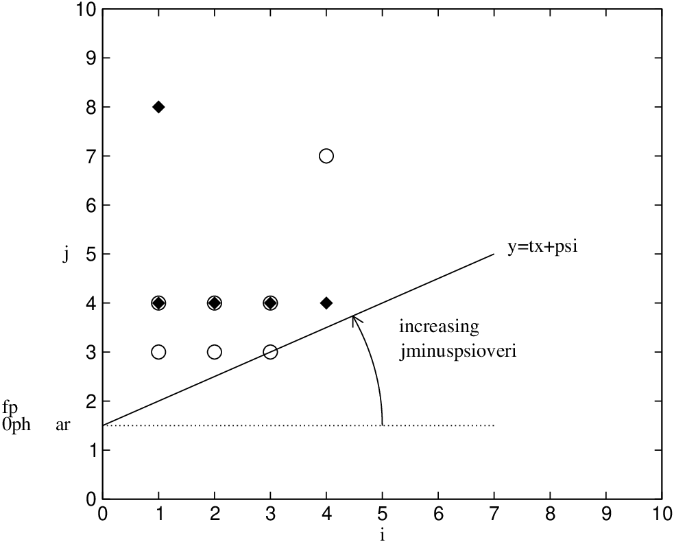
Fig. 2: Diagram of the VN input-output weight enumerating functions and growth rate dominant set in the (i,j)(i,j) plane. The illustration is for a smallest CN minimum distance of r=3r=3, so ψ=3/2\psi=3/2. The sets St−S_{t}^{-} for the two VN types t∈Iv={1,2}t\in I_{v}=\{1,2\} are illustrated by open circles and filled diamonds respectively. The line ℒ\mathcal{L} has a fixed point at (0,ψ)(0,\psi) and is rotated in an anticlockwise fashion until it touches any of these points. In this example, this occurs at the point (3,3)∈S1−(3,3)\in S_{1}^{-}. Therefore in this example T=1/2T=1/2, Yv={1}Y_{v}=\{1\}, P1={(3,3)}P_{1}=\{(3,3)\} and for small values of α\alpha the dominating contribution to the growth rate comes from weight-33 local codewords of the type-11 VNs generated by weight-33 local input words.

From Theorem 28 and from the definitions of Q1​(x)Q_{1}(x) and Q2​(x)Q_{2}(x) given in (22) and (23) respectively, we observe that the triples (t,i,j)(t,i,j) (or, equivalently, VN input-output weight enumerating function coefficients Bi,j(t)B^{(t)}_{i,j}) such that (i,j)(i,j) lies in one of the sets PtP_{t} (t∈Yvt\in Y_{v}) make a dominating contribution to the growth rate for values of α\alpha close to zero. We will refer to the set of such triples as the dominant set. Note that the dominant set may equivalently be described as the set of triples (t,i,j)(t,i,j) such that Ti,j=TT_{i,j}=T for some t∈Ivt\in I_{v}, (i,j)∈St−(i,j)\in S_{t}^{-}.

Interestingly, the dominant set admits an instructive graphical interpretation and may be easily identified using a very simple geometric construction. In the (i,j)(i,j) plane, a line ℒ\mathcal{L} through the fixed point (0,ψ)(0,\psi) is rotated in an anticlockwise fashion until it comes in contact with one or more of the points (i,j)∈S−(i,j)\in S^{-}. The slope of the line ℒ\mathcal{L} at this point is the parameter TT defined in (19), the set of t∈Ivt\in I_{v} which have points (i,j)∈ℒ(i,j)\in\mathcal{L} is the set defined as YvY_{v}, and for each such tt the set of such points on ℒ\mathcal{L} is the set PtP_{t} defined in (21). Note that due to (14), the position of the fixed point (0,ψ)(0,\psi) depends only on the smallest CN minimum distance rr, and always lies somewhere on the line segment joining (0,1)(0,1) and (0,2)(0,2), including the latter endpoint.

This interpretation is illustrated in Fig. 2 for an example D-GLDPC code with two VN types Iv={1,2}I_{v}=\{1,2\}. Type 1∈Iv1\in I_{v} (open circles) corresponds to the Hamming code of length q1=7q_{1}=7, dimension k1=4k_{1}=4, minimum distance p1=3p_{1}=3 and represented by the systematic generator matrix 𝐆𝖧=[1000111,0100110,0010101,0001011]\mathbf{G}_{\mathsf{H}}=[1000111,0100110,0010101,0001011]. Type 2∈Iv2\in I_{v} (filled diamonds) corresponds to the first-order Reed-Muller code of length q2=8q_{2}=8, dimension k2=4k_{2}=4, minimum distance p2=4p_{2}=4 and represented by the generator matrix 𝐆𝖱𝖬=[11111111,11110000,11001100,10101010]\mathbf{G}_{\mathsf{RM}}=[11111111,11110000,11001100,10101010]. In the specific case of Fig. 2 we have ψ=3/2\psi=3/2, which corresponds to r=3r=3.22 2 For example, assuming a uniform CN set composed of (15,11)(15,11) Hamming codes, and assuming λ1=7/15\lambda_{1}=7/15 and λ2=8/15\lambda_{2}=8/15, through (7) this would represent a rate R=1/2R=1/2 ensemble. It may be deduced from the figure that for values of α\alpha close to zero the growth rate G⁡(α)G(\alpha) is dominated by weight-33 local codewords of the Hamming VNs associated with weight-33 local input words.

From Corollary 35 we observe that in the special case where r=p=2r=p=2, the growth rate depends only on the CN and VN with minimum distance equal to 22, and (34) is a first-order Taylor series around α=0\alpha=0 which directly generalizes the results of [11] and [15] (for irregular LDPC and GLDPC codes respectively) to the case of irregular D-GLDPC codes. Note that the error term in (34) is O⁡(αξ)O(\alpha^{\xi}), which is different to the error term O⁡(α2)O(\alpha^{2}) reported in previous literature (Theorem 4.1 in [24], Theorem 5 in [11]); this difference is manifest in the case where r=p=2r=p=2 and either r¯=3\bar{r}=3 or p¯=3\bar{p}=3. Corollary 35 indicates that in the analysis of the asymptotic growth rate of the weight distribution, the parameter 1/P−1​(1/C)1/P^{-1}(1/C) in the context of D-GLDPC codes plays an analagous role to the parameter λ′​(0)​ρ′​(1)\lambda^{\prime}(0)\rho^{\prime}(1) for irregular LDPC codes, and to the parameter λ′​(0)​C\lambda^{\prime}(0)C for irregular GLDPC codes. It discriminates between ensemble sequences with good growth rate behavior, for which 1/P−1​(1/C)<11/P^{-1}(1/C)<1, and ensemble sequences with bad growth rate behavior, for which 1/P−1​(1/C)>11/P^{-1}(1/C)>1.

V Proof of the Main Result

In this section, Theorem 28 is proved. For ease of presentation, the proof is broken into four parts.

V-A Number of check-valid assignments of weight ϵ​m\epsilon m over γ​m\gamma m CN of type t∈Ict\in I_{c}

Consider γ​m\gamma m CN of the same type t∈Ict\in I_{c}. Using generating functions, the number of check-valid assignments (over these CN) of weight ϵ​m\epsilon m is given by33 3 Here we make use of the following general result [25]. Let aia_{i} be the number of ways of obtaining an outcome i∈ℤi\in\mathbb{Z} in experiment 𝒜{\mathcal{A}}, and let bjb_{j} be the number of ways of obtaining an outcome j∈ℤj\in\mathbb{Z} in experiment ℬ{\mathcal{B}}. Also let ckc_{k} be the number of ways of obtaining an outcome (i,j)(i,j) in the combined experiment (𝒜,ℬ)({\mathcal{A}},{\mathcal{B}}) with sum i+j=ki+j=k. Then the generating functions A⁡(x)=∑iai​xiA(x)=\sum_{i}a_{i}x^{i}, B⁡(x)=∑jbj​xjB(x)=\sum_{j}b_{j}x^{j} and C⁡(x)=∑kck​xkC(x)=\sum_{k}c_{k}x^{k} are related by C⁡(x)=A⁡(x)​B​(x)C(x)=A(x)B(x).

Nc,t(γ​m)​(ϵ​m)=Coeff ​[(A(t)​(x))γ​m,xϵ​m]N_{c,t}^{(\gamma m)}(\epsilon m)={\mbox{Coeff }}\left[\left(A^{(t)}(x)\right)^{\gamma m},x^{\epsilon m}\right]

where Coeff ​[p​(x),xc]{\mbox{Coeff }}[p(x),x^{c}] denotes the coefficient of xcx^{c} in the polynomial p⁡(x)p(x). We now use the following result, the proof of which appears in [10, Appendix A]:

Lemma V.1

Let A⁡(x)=1+∑u=cdAu​xuA(x)=1+\sum_{u=c}^{d}A_{u}x^{u}, where 1≤c≤d1\leq c\leq d, be a polynomial satisfying Ac>0A_{c}>0 and Au≥0A_{u}\geq 0 for all c<u≤dc<u\leq d. For a fixed positive rational number ξ\xi, consider the set of positive integers ℓ\ell such that ξ​ℓ∈ℕ\xi\ell\in\mathbb{N} and Coeff ​[(A⁡(x))ℓ,xξ​ℓ]>0{\mbox{Coeff }}[\left(A(x)\right)^{\ell},x^{\xi\ell}]>0. Then either this set is empty, or it has infinite cardinality; if tt is one such ℓ\ell, then so is j​tjt for every positive integer jj. In the latter case, the following limit is well defined and exists:

limℓ→∞1ℓ​log⁡Coeff ​[(A⁡(x))ℓ,xξ​ℓ]=max⁡∑i∈U𝜷⁡βi​log⁡(Aiβi)\lim_{\ell\rightarrow\infty}\frac{1}{\ell}\log{\mbox{Coeff }}\left[\left(A(x)\right)^{\ell},x^{\xi\ell}\right]=\max_{{\mbox{\scriptsize\boldmath$\beta$}}}\sum_{i\in U}\beta_{i}\log\left(\frac{A_{i}}{\beta_{i}}\right) (37)

where U={i∈ℕ:Ai>0}U=\{i\in\mathbb{N}\;:\;A_{i}>0\}, 𝛃=(βi)i∈U{\mbox{\boldmath$\beta$}}=(\beta_{i})_{i\in U}, and the maximization is subject to the constraints ∑i∈Uβi=1\sum_{i\in U}\beta_{i}=1, ∑i∈Ui​βi=ξ\sum_{i\in U}i\beta_{i}=\xi and βi≥0\beta_{i}\geq 0 for all i∈Ui\in U.

Applying this lemma by substituting A​(x)=A(t)​(x)A(x)=A^{(t)}(x), ℓ=γ​m\ell=\gamma m and ξ=ϵ/γ\xi=\epsilon/\gamma, we obtain that with γ\gamma fixed, as m→∞m\rightarrow\infty

Nc,t(γ​m)​(ϵ​m)=Coeff ​[(A(t)​(x))γ​m,xϵ​m]\displaystyle N_{c,t}^{(\gamma m)}(\epsilon m)={\mbox{Coeff }}\left[\left(A^{(t)}(x)\right)^{\gamma m},x^{\epsilon m}\right] (38)
≈mexp⁡{m​γ​max⁡∑i∈Ut𝜷(t)⁡βi(t)​log⁡(Ai(t)βi(t))}\displaystyle\stackrel{{\scriptstyle m}}{{\approx}}\exp\left\{m\gamma\max_{{\mbox{\scriptsize\boldmath$\beta$}}^{(t)}}\sum_{i\in U_{t}}\beta^{(t)}_{i}\log\left(\frac{A^{(t)}_{i}}{\beta^{(t)}_{i}}\right)\right\} (39)
≜exp⁡{m​Wt(γ)​(ϵ)}\displaystyle\triangleq\exp\left\{mW^{(\gamma)}_{t}(\epsilon)\right\} (40)

where the maximization over 𝜷(t)=(βi(t))i∈Ut{\mbox{\boldmath$\beta$}}^{(t)}=(\beta^{(t)}_{i})_{i\in U_{t}} is subject to the constraints ∑i∈Utβi(t)=1\sum_{i\in U_{t}}\beta^{(t)}_{i}=1, ∑i∈Ut−i​βi(t)=ϵ/γ\sum_{i\in U_{t}^{-}}i\beta^{(t)}_{i}=\epsilon/\gamma and βi(t)≥0\beta^{(t)}_{i}\geq 0 for all i∈Uti\in U_{t} (recall that the sets UtU_{t} and Ut−U_{t}^{-} are given by (9) and (10)).

V-B Number of check-valid assignments of weight δ​m\delta m

Next we derive an expression, valid asymptotically, for the number of check-valid assignments of weight δ​m\delta m. For each t∈Ict\in I_{c}, let ϵt​m\epsilon_{t}m denote the portion of the total weight δ​m\delta m apportioned to CN of type tt. Then ϵt≥0\epsilon_{t}\geq 0 for each t∈Ict\in I_{c}, and ∑t∈Icϵt=δ\sum_{t\in I_{c}}\epsilon_{t}=\delta. Also denote ϵ=(ϵ1ϵ2⋯ϵnc){\mbox{\boldmath$\epsilon$}}=(\epsilon_{1}\;\epsilon_{2}\;\cdots\;\epsilon_{n_{c}}). The number of check-valid assignments of weight δ​m\delta m satisfying the constraint ϵ\epsilon is obtained by multiplying the numbers of check-valid assignments of weight ϵt​m\epsilon_{t}m over γt​m\gamma_{t}m CN of type tt, for each t∈Ict\in I_{c},

Nc(ϵ)​(δ​m)=∏t∈IcNc,t(γt​m)​(ϵt​m)N_{c}^{({\mbox{\boldmath$\epsilon$}})}(\delta m)=\prod_{t\in I_{c}}N_{c,t}^{(\gamma_{t}m)}(\epsilon_{t}m) (41)

where the fraction γt\gamma_{t} of CN of type t∈Ict\in I_{c} is given by (4).

The number of check-valid assignments of weight δ​m\delta m, which we denote Nc​(δ​m)N_{c}(\delta m), is equal to the sum of Nc(ϵ)​(δ​m)N_{c}^{({\mbox{\boldmath$\epsilon$}})}(\delta m) over all admissible vectors ϵ\epsilon; therefore, as m→∞m\rightarrow\infty

Nc(δm)≈m∑ϵ:∑t∈Icϵt=δexp{m∑t∈IcWt(γt)(ϵt)}N_{c}(\delta m)\,\stackrel{{\scriptstyle m}}{{\approx}}\sum_{{\mbox{\scriptsize\boldmath$\epsilon$}}\;:\;\sum_{t\in I_{c}}\epsilon_{t}=\delta}\exp\left\{m\sum_{t\in I_{c}}W^{(\gamma_{t})}_{t}(\epsilon_{t})\right\} (42)

where we have used (40) and (41). However, the asymptotic expression as m→∞m\rightarrow\infty is dominated by the distribution ϵ\epsilon which maximizes the argument of the exponential44 4 Observe that as m→∞m\rightarrow\infty, ∑texp⁡(m​Zt)≈mexp⁡(m​maxt​{Zt})\sum_{t}\exp(mZ_{t})\stackrel{{\scriptstyle m}}{{\approx}}\exp(m\max_{t}\{Z_{t}\}). Therefore as m→∞m\rightarrow\infty

Nc​(δ​m)≈mexp⁡{m​W}N_{c}(\delta m)\stackrel{{\scriptstyle m}}{{\approx}}\exp\left\{mW\right\} (43)

where

W=max⁡∑t∈Icϵ⁡γt​max⁡∑i∈Ut𝜷(t)⁡βi(t)​log⁡(Ai(t)βi(t)),W=\max_{{\mbox{\scriptsize\boldmath$\epsilon$}}}\sum_{t\in I_{c}}\gamma_{t}\max_{{\mbox{\scriptsize\boldmath$\beta$}}^{(t)}}\sum_{i\in U_{t}}\beta^{(t)}_{i}\log\left(\frac{A^{(t)}_{i}}{\beta^{(t)}_{i}}\right)\;, (44)

the maximization over ϵ\epsilon is subject to the constraint

∑t∈Icϵt=δ,\sum_{t\in I_{c}}\epsilon_{t}=\delta\;, (45)

and for each t∈Ict\in I_{c} the maximization over 𝜷(t)=(βi(t))i∈Ut{\mbox{\boldmath$\beta$}}^{(t)}=(\beta^{(t)}_{i})_{i\in U_{t}} is subject to the constraints

∑i∈Utβi(t)=1\sum_{i\in U_{t}}\beta^{(t)}_{i}=1 (46)
∑i∈Ut−i​βi(t)=ϵt/γt\sum_{i\in U_{t}^{-}}i\beta^{(t)}_{i}=\epsilon_{t}/\gamma_{t} (47)

and

βi(t)≥0∀i∈Ut.\beta^{(t)}_{i}\geq 0\quad\forall i\in U_{t}\;. (48)

Next, for each t∈Ict\in I_{c} we define

Ft​(𝜷(t))=β0(t)​log⁡(1β0(t))−∑i∈Ut−βi(t).F_{t}({\mbox{\boldmath$\beta$}}^{(t)})=\beta^{(t)}_{0}\log\left(\frac{1}{\beta^{(t)}_{0}}\right)-\sum_{i\in U_{t}^{-}}\beta^{(t)}_{i}\;.

We then have the following lemma.

Lemma V.2

The expression ∑t∈Icγt​Ft​(𝛃(t))\sum_{t\in I_{c}}\gamma_{t}F_{t}({\mbox{\boldmath$\beta$}}^{(t)}) is O⁡(δ2)O(\delta^{2}) for any 𝛃(t){\mbox{\boldmath$\beta$}}^{(t)} satisfying the optimization constraints (45)–(48).

A proof of this lemma is given in Appendix A. It follows from Lemma V.2 that the expression ∑t∈Icγt​Ft​(𝜷(t))\sum_{t\in I_{c}}\gamma_{t}F_{t}({\mbox{\boldmath$\beta$}}^{(t)}) is O⁡(δ2)O(\delta^{2}) for the maximizing 𝜷(t){\mbox{\boldmath$\beta$}}^{(t)}. Therefore

W\displaystyle W =\displaystyle= max⁡∑t∈Icϵ⁡γt​max𝜷(t)​[∑i∈Ut−βi(t)​log⁡(e​Ai(t)βi(t))+Ft​(𝜷(t))]\displaystyle\max_{{\mbox{\scriptsize\boldmath$\epsilon$}}}\sum_{t\in I_{c}}\gamma_{t}\max_{{\mbox{\scriptsize\boldmath$\beta$}}^{(t)}}\left[\sum_{i\in U_{t}^{-}}\beta^{(t)}_{i}\log\left(\frac{eA^{(t)}_{i}}{\beta^{(t)}_{i}}\right)+F_{t}({\mbox{\boldmath$\beta$}}^{(t)})\right]
=\displaystyle= max⁡∑t∈Icϵ⁡γt​max⁡∑i∈Ut−𝜷(t)⁡βi(t)​log⁡(e​Ai(t)βi(t))+O⁡(δ2)\displaystyle\max_{{\mbox{\scriptsize\boldmath$\epsilon$}}}\sum_{t\in I_{c}}\gamma_{t}\max_{{\mbox{\scriptsize\boldmath$\beta$}}^{(t)}}\sum_{i\in U_{t}^{-}}\beta^{(t)}_{i}\log\left(\frac{eA^{(t)}_{i}}{\beta^{(t)}_{i}}\right)+O(\delta^{2})

where the maximization over 𝜷(t)=(βi(t))i∈Ut−{\mbox{\boldmath$\beta$}}^{(t)}=(\beta^{(t)}_{i})_{i\in U_{t}^{-}} (for each t∈Ict\in I_{c}) is subject to the constraint (47) together with βi(t)≥0\beta^{(t)}_{i}\geq 0 for all i∈Ut−i\in U_{t}^{-}. In what follows, for convenience of presentation we shall temporarily omit the O⁡(δ2)O(\delta^{2}) term in the expression for WW.

Next we make the substitution θi(t)=γt​βi(t)\theta^{(t)}_{i}=\gamma_{t}\beta^{(t)}_{i} for all t∈Ict\in I_{c}, i∈Ut−i\in U_{t}^{-}. This yields

W=max⁡∑t∈Icϵ⁡max⁡∑i∈Ut−𝜽(t)⁡θi(t)​log⁡(e​Ai(t)​γtθi(t))W=\max_{{\mbox{\scriptsize\boldmath$\epsilon$}}}\sum_{t\in I_{c}}\max_{{\mbox{\scriptsize\boldmath$\theta$}}^{(t)}}\sum_{i\in U_{t}^{-}}\theta^{(t)}_{i}\log\left(\frac{eA^{(t)}_{i}\gamma_{t}}{\theta^{(t)}_{i}}\right)

where the maximization over 𝜽(t)=(θi(t))i∈Ut−{\mbox{\boldmath$\theta$}}^{(t)}=(\theta^{(t)}_{i})_{i\in U_{t}^{-}} (for each t∈Ict\in I_{c}) is subject to the constraints ∑i∈Ut−i​θi(t)=ϵt\sum_{i\in U_{t}^{-}}i\theta^{(t)}_{i}=\epsilon_{t} and θi(t)≥0\theta^{(t)}_{i}\geq 0 for all i∈Ut−i\in U_{t}^{-}. We observe that this maximization may be recast as

W=max𝜽∑t∈Ic∑i∈Ut−θi(t)log(e​Ai(t)​γtθi(t))W=\max_{{\mbox{\scriptsize\boldmath$\theta$}}}\sum_{t\in I_{c}}\sum_{i\in U_{t}^{-}}\theta^{(t)}_{i}\log\left(\frac{eA^{(t)}_{i}\gamma_{t}}{\theta^{(t)}_{i}}\right)

where by (45) the maximization, which is now over 𝜽=(θi(t))t∈Ic,i∈Ut−{\mbox{\boldmath$\theta$}}=(\theta^{(t)}_{i})_{t\in I_{c},i\in U_{t}^{-}}, is subject to the constraints

∑t∈Ic∑i∈Ut−i​θi(t)=δ\sum_{t\in I_{c}}\sum_{i\in U_{t}^{-}}i\theta^{(t)}_{i}=\delta

and θi(t)≥0\theta^{(t)}_{i}\geq 0 for all t∈Ict\in I_{c}, i∈Ut−i\in U_{t}^{-}.

Making the substitution υi(t)=θi(t)/δ\upsilon^{(t)}_{i}=\theta^{(t)}_{i}/\delta for all t∈Ict\in I_{c}, i∈Ut−i\in U_{t}^{-}, we obtain

W=δ​max𝝊​∑t∈Ic∑i∈Ut−υi(t)​log⁡(e​Ai(t)​γtδ​υi(t))W=\delta\max_{{\mbox{\scriptsize\boldmath$\upsilon$}}}\sum_{t\in I_{c}}\sum_{i\in U_{t}^{-}}\upsilon^{(t)}_{i}\log\left(\frac{eA^{(t)}_{i}\gamma_{t}}{\delta\upsilon^{(t)}_{i}}\right) (49)

where the maximization over 𝝊=(υi(t))t∈Ic,i∈Ut−{\mbox{\boldmath$\upsilon$}}=(\upsilon^{(t)}_{i})_{t\in I_{c},i\in U_{t}^{-}} is subject to the constraints

∑t∈Ic∑i∈Ut−i​υi(t)=1\sum_{t\in I_{c}}\sum_{i\in U_{t}^{-}}i\upsilon^{(t)}_{i}=1 (50)

and υi(t)≥0\upsilon^{(t)}_{i}\geq 0 for all t∈Ict\in I_{c}, i∈Ut−i\in U_{t}^{-}.

Solving the constrained optimization (49) using Lagrange multipliers yields

υi(t)=Ai(t)​γtδ​e−i​λ∀t∈Ic,i∈Ut−,\upsilon_{i}^{(t)}=\frac{A_{i}^{(t)}\gamma_{t}}{\delta}e^{-i\lambda}\quad\forall t\in I_{c},i\in U_{t}^{-}\;, (51)

where λ\lambda is the Lagrange multiplier. Substituting (51) into (50) and defining z=e−λz=e^{-\lambda} yields

∑t∈Ic∑i∈Ut−i​Ai(t)​γt​zi=δ.\sum_{t\in I_{c}}\sum_{i\in U_{t}^{-}}iA_{i}^{(t)}\gamma_{t}z^{i}=\delta\,. (52)

We may write this as

∑t∈Xcr​Ar(t)​γt​zr+∑t∈Ic∑i∈Ut−\{r}i​Ai(t)​γt​zi=δ\sum_{t\in X_{c}}rA_{r}^{(t)}\gamma_{t}z^{r}+\sum_{t\in I_{c}}\sum_{i\in U_{t}^{-}\backslash\{r\}}iA_{i}^{(t)}\gamma_{t}z^{i}=\delta (53)

from which we obtain (since all coefficients are positive and z=e−λ>0z=e^{-\lambda}>0)

∑t∈Xcr​Ar(t)​γt​zr≤δ\sum_{t\in X_{c}}rA_{r}^{(t)}\gamma_{t}z^{r}\leq\delta

and therefore

z≤1(∑t∈Xcr​Ar(t)​γt)1/r​δ1/rz\leq\frac{1}{\left(\sum_{t\in X_{c}}rA_{r}^{(t)}\gamma_{t}\right)^{1/r}}\,\delta^{1/r} (54)

is valid for all δ>0\delta>0. Thus

z∼O⁡(δ1/r).z\sim O(\delta^{1/r})\;. (55)

Recalling the definition z=e−λz=e^{-\lambda}, (51) and (55) together imply that

υi(t)∼O⁡(δi/r−1)∀t∈Ic,i∈Ut−.\upsilon^{(t)}_{i}\sim O\left(\delta^{i/r-1}\right)\quad\forall t\in I_{c},i\in U_{t}^{-}\;. (56)

Next, since the value of 𝝊\upsilon which achieves the maximum in (49) satisfies (51), we may develop (49) as

W\displaystyle W =\displaystyle= δ​∑t∈Ic∑i∈Ut−υi(t)​(1+i​λ)\displaystyle\delta\sum_{t\in I_{c}}\sum_{i\in U_{t}^{-}}\upsilon_{i}^{(t)}(1+i\lambda) (57)
=\displaystyle= δ⁡(∑t∈Ic∑i∈Ut−υi(t)+λ)\displaystyle\delta\left(\sum_{t\in I_{c}}\sum_{i\in U_{t}^{-}}\upsilon_{i}^{(t)}+\lambda\right) (58)

where in the second line we have used the constraint (50).

Now, the constraint (50) may be written as

1=∑t∈Ic∑i∈Ut−rυi(t)+∑t,i:i>r(i−r)υi(t)1=\sum_{t\in I_{c}}\sum_{i\in U_{t}^{-}}r\upsilon_{i}^{(t)}+\sum_{t,i\;:\;i>r}(i-r)\upsilon_{i}^{(t)}

so

∑t∈Ic∑i∈Ut−υi(t)=1r−1r∑t,i:i>r(i−r)υi(t).\sum_{t\in I_{c}}\sum_{i\in U_{t}^{-}}\upsilon_{i}^{(t)}=\frac{1}{r}-\frac{1}{r}\sum_{t,i\;:\;i>r}(i-r)\upsilon_{i}^{(t)}\;. (59)

Also, we may write by (51)

δ​υr(t)​er​λ=Ar(t)​γt,∀t∈Xc.\delta\upsilon_{r}^{(t)}e^{r\lambda}=A_{r}^{(t)}\gamma_{t}\;,\quad\forall t\in X_{c}\;.

Multiplying by rr and summing over all t∈Xct\in X_{c} yields

δ​er​λ​∑t∈Xcr​υr(t)=∑t∈Xcr​Ar(t)​γt.\delta e^{r\lambda}\sum_{t\in X_{c}}r\upsilon_{r}^{(t)}=\sum_{t\in X_{c}}rA_{r}^{(t)}\gamma_{t}\;.

Extracting λ\lambda yields

λ\displaystyle\lambda =\displaystyle= 1r​log⁡(∑t∈Xcr​Ar(t)​γtδ​∑t∈Xcr​υr(t))\displaystyle\frac{1}{r}\log\left(\frac{\sum_{t\in X_{c}}rA_{r}^{(t)}\gamma_{t}}{\delta\sum_{t\in X_{c}}r\upsilon_{r}^{(t)}}\right) (60)
=\displaystyle= 1r​log⁡(∑t∈Xcr​Ar(t)​γtδ)−1r​log⁡(∑t∈Xcr​υr(t))\displaystyle\frac{1}{r}\log\left(\frac{\sum_{t\in X_{c}}rA_{r}^{(t)}\gamma_{t}}{\delta}\right)-\frac{1}{r}\log\left(\sum_{t\in X_{c}}r\upsilon_{r}^{(t)}\right)
=\displaystyle= 1rlog(∑t∈Xcr​Ar(t)​γtδ)−1rlog(1−∑t,i:i>riυi(t)).\displaystyle\frac{1}{r}\log\left(\frac{\sum_{t\in X_{c}}rA_{r}^{(t)}\gamma_{t}}{\delta}\right)-\frac{1}{r}\log\left(1-\sum_{t,i\;:\;i>r}i\upsilon_{i}^{(t)}\right)\;.

where we have used (50) in the final line. Substituting (59) and (60) back into (58) yields

W\displaystyle W =\displaystyle= (δr)log(e​∑t∈Xcr​Ar(t)​γtδ)−(δr)[∑t,i:i>r(i−r)υi(t)+log(1−∑t,i:i>riυi(t))]\displaystyle\left(\frac{\delta}{r}\right)\log\left(\frac{e\sum_{t\in X_{c}}rA_{r}^{(t)}\gamma_{t}}{\delta}\right)-\left(\frac{\delta}{r}\right)\left[\sum_{t,i\;:\;i>r}(i-r)\upsilon_{i}^{(t)}+\log\left(1-\sum_{t,i\;:\;i>r}i\upsilon_{i}^{(t)}\right)\right]
=\displaystyle= (δr)log(e​Cδ​∫ρ)−(δr)[∑t,i:i>r(i−r)υi(t)+log(1−∑t,i:i>riυi(t))]\displaystyle\left(\frac{\delta}{r}\right)\log\left(\frac{eC}{\delta\int\rho}\right)-\left(\frac{\delta}{r}\right)\left[\sum_{t,i\;:\;i>r}(i-r)\upsilon_{i}^{(t)}+\log\left(1-\sum_{t,i\;:\;i>r}i\upsilon_{i}^{(t)}\right)\right]
=\displaystyle= (δr)​log⁡(e​Cδ​∫ρ)+O⁡(δr¯/r)\displaystyle\left(\frac{\delta}{r}\right)\log\left(\frac{eC}{\delta\int\rho}\right)+O(\delta^{\bar{r}/r})

where in the second line we have used (15), and in the final line we have used (56) and the fact that log⁡(1+α)∼O⁡(α)\log(1+\alpha)\sim O(\alpha) (also recall the definition (16)).

Substituting this expression for WW into (43) while recalling the O⁡(δ2)O(\delta^{2}) term in the expression for WW, we have that as m→∞m\rightarrow\infty

Nc​(δ​m)≈mexp⁡{m⁡[δr​log⁡(e​Cδ​∫ρ)+O⁡(δmin⁡{r¯/r,2})]}.N_{c}(\delta m)\stackrel{{\scriptstyle m}}{{\approx}}\exp\left\{m\left[\frac{\delta}{r}\log\left(\frac{eC}{\delta\int\rho}\right)+O\left(\delta^{\min\{\bar{r}/r,2\}}\right)\right]\right\}\;. (61)

Note that (61) generalizes [11, eqn. (30)] to the case of a generalized CN set.

V-C Number of variable-valid split assignments of split weight (τ​n,σ​n)(\tau n,\sigma n) over γ​n\gamma n VN of type t∈Ivt\in I_{v}

Consider γ​n\gamma n VN of the same type t∈Ivt\in I_{v}. We now evaluate the number of variable-valid split assignments (over these VN) of split weight (τ​n,σ​n)(\tau n,\sigma n). Using generating functions, this is given by55 5 We use the following result on bivariate generating functions [25]. Let ai,ja_{i,j} be the number of ways of obtaining an outcome (i,j)∈ℤ2(i,j)\in\mathbb{Z}^{2} in experiment 𝒜{\mathcal{A}}, and let bk,lb_{k,l} be the number of ways of obtaining an outcome (k,l)∈ℤ2(k,l)\in\mathbb{Z}^{2} in experiment ℬ{\mathcal{B}}. Also let cp,qc_{p,q} be the number of ways of obtaining an outcome ((i,j),(k,l))((i,j),(k,l)) in the combined experiment (𝒜,ℬ)({\mathcal{A}},{\mathcal{B}}) with sums i+k=pi+k=p and j+l=qj+l=q. Then the generating functions A⁡(x,y)=∑i,jai,j​xi​yjA(x,y)=\sum_{i,j}a_{i,j}x^{i}y^{j}, B⁡(x,y)=∑k,lbk,l​xk​ylB(x,y)=\sum_{k,l}b_{k,l}x^{k}y^{l} and C⁡(x,y)=∑p,qcp,q​xp​yqC(x,y)=\sum_{p,q}c_{p,q}x^{p}y^{q} are related by C⁡(x,y)=A⁡(x,y)​B​(x,y)C(x,y)=A(x,y)B(x,y).

Nv,t(γ​n)​(τ​n,σ​n)=Coeff ​[(B(t)​(x,y))γ​n,xτ​n​yσ​n]N_{v,t}^{(\gamma n)}(\tau n,\sigma n)={\mbox{Coeff }}\left[\left(B^{(t)}(x,y)\right)^{\gamma n},x^{\tau n}y^{\sigma n}\right]

where Coeff ​[p⁡(x,y),xc​yd]{\mbox{Coeff }}[p(x,y),x^{c}y^{d}] denotes the coefficient of xc​ydx^{c}y^{d} in the bivariate polynomial p⁡(x,y)p(x,y). We make use of the following result, the proof of which appears in [10, Appendix A]:

Lemma V.3

Let

B⁡(x,y)=1+∑u=1k∑v=cdBu,v​xu​yvB(x,y)=1+\sum_{u=1}^{k}\sum_{v=c}^{d}B_{u,v}x^{u}y^{v}

where k≥1k\geq 1 and 1≤c≤d1\leq c\leq d, be a bivariate polynomial satisfying Bu,v≥0B_{u,v}\geq 0 for all 1≤u≤k1\leq u\leq k, c≤v≤dc\leq v\leq d. For fixed positive rational numbers ξ\xi and θ\theta, consider the set of positive integers ℓ\ell such that ξ​ℓ∈ℕ\xi\ell\in\mathbb{N}, θ​ℓ∈ℕ\theta\ell\in\mathbb{N} and Coeff ​[(B⁡(x,y))ℓ,xξ​ℓ​yθ​ℓ]>0{\mbox{Coeff }}[(B(x,y))^{\ell},x^{\xi\ell}y^{\theta\ell}]>0. Then either this set is empty, or has infinite cardinality; if tt is one such ℓ\ell, then so is j​tjt for every positive integer jj. Assuming the latter case, the following limit is well defined and exists:

limℓ→∞1ℓ​log⁡Coeff ​[(B⁡(x,y))ℓ,xξ​ℓ​yθ​ℓ]=max⁡∑(i,j)∈S𝜼⁡ηi,j​log⁡(Bi,jηi,j)\lim_{\ell\rightarrow\infty}\frac{1}{\ell}\log{\mbox{Coeff }}\left[\left(B(x,y)\right)^{\ell},x^{\xi\ell}y^{\theta\ell}\right]=\max_{{\mbox{\scriptsize\boldmath$\eta$}}}\sum_{(i,j)\in S}\eta_{i,j}\log\left(\frac{B_{i,j}}{\eta_{i,j}}\right) (62)

where S={(i,j)∈ℕ2:Bi,j>0}S=\{(i,j)\in\mathbb{N}^{2}\;:\;B_{i,j}>0\}, 𝛈=(ηi,j)(i,j)∈S{\mbox{\boldmath$\eta$}}=(\eta_{i,j})_{(i,j)\in S}, and the maximization is subject to the constraints ∑(i,j)∈Sηi,j=1\sum_{(i,j)\in S}\eta_{i,j}=1, ∑(i,j)∈Si​ηi,j=ξ\sum_{(i,j)\in S}i\eta_{i,j}=\xi, ∑(i,j)∈Sj​ηi,j=θ\sum_{(i,j)\in S}j\eta_{i,j}=\theta and ηi,j≥0\eta_{i,j}\geq 0 for all (i,j)∈S(i,j)\in S.

Applying this lemma by substituting B⁡(x,y)=B(t)​(x,y)B(x,y)=B^{(t)}(x,y), ℓ=γ​n\ell=\gamma n, ξ=τ/γ\xi=\tau/\gamma and θ=σ/γ\theta=\sigma/\gamma, we obtain that with γ\gamma fixed, as n→∞n\rightarrow\infty

Nv,t(γ​n)​(τ​n,σ​n)=Coeff ​[(B(t)​(x,y))γ​n,xτ​n​yσ​n]\displaystyle N_{v,t}^{(\gamma n)}(\tau n,\sigma n)={\mbox{Coeff }}\left[\left(B^{(t)}(x,y)\right)^{\gamma n},x^{\tau n}y^{\sigma n}\right] (63)
≈nexp⁡{n​γ​max⁡∑(i,j)∈St𝜼(t)⁡ηi,j(t)​log⁡(Bi,j(t)ηi,j(t))}\displaystyle\stackrel{{\scriptstyle n}}{{\approx}}\exp\left\{n\gamma\max_{{\mbox{\scriptsize\boldmath$\eta$}}^{(t)}}\sum_{(i,j)\in S_{t}}\eta^{(t)}_{i,j}\log\left(\frac{B^{(t)}_{i,j}}{\eta^{(t)}_{i,j}}\right)\right\} (64)
≜exp⁡{n​Xt(γ)​(τ,σ)}\displaystyle\triangleq\exp\left\{nX^{(\gamma)}_{t}(\tau,\sigma)\right\} (65)

where the maximization over 𝜼(t)=(ηi,j(t))(i,j)∈St{\mbox{\boldmath$\eta$}}^{(t)}=(\eta^{(t)}_{i,j})_{(i,j)\in S_{t}} is subject to the constraints ∑(i,j)∈Stηi,j(t)=1\sum_{(i,j)\in S_{t}}\eta^{(t)}_{i,j}=1, ∑(i,j)∈St−i​ηi,j(t)=τ/γ\sum_{(i,j)\in S_{t}^{-}}i\eta^{(t)}_{i,j}=\tau/\gamma, ∑(i,j)∈St−j​ηi,j(t)=σ/γ\sum_{(i,j)\in S_{t}^{-}}j\eta^{(t)}_{i,j}=\sigma/\gamma and ηi,j(t)≥0\eta^{(t)}_{i,j}\geq 0 for all (i,j)∈St(i,j)\in S_{t} (recall that the sets StS_{t} and St−S_{t}^{-} are given by (11) and (12)).

V-D Growth rate of the weight distribution of the irregular D-GLDPC code ensemble sequence

Recall that the number of check-valid assignments of weight δ​m\delta m is Nc​(δ​m)N_{c}(\delta m); also, the total number of assignments of weight δ​m\delta m is (Eδ​m)\binom{E}{\delta m}. Therefore, the probability that a randomly chosen assignment of weight δ​m\delta m is check-valid is given by

Pvalid​(δ​m)=Nc​(δ​m)/(Eδ​m).P_{\mbox{\scriptsize valid}}(\delta m)=N_{c}(\delta m)\Big/\binom{E}{\delta m}\;.

Here we adopt the notation δ​m=β​n\delta m=\beta n; also we have E=m/∫ρ=n/∫λE=m/\int\rho=n/\int\lambda. The binomial coefficient may be asymptotically approximated using the fact, based on Stirling’s approximation, that as n→∞n\rightarrow\infty [11]

(τ​nσ​n)≈nexp⁡{n⁡[σ​log⁡(e​τσ)+O⁡(σ2)]}\binom{\tau n}{\sigma n}\stackrel{{\scriptstyle n}}{{\approx}}\exp\left\{n\left[\sigma\log\left(\frac{e\tau}{\sigma}\right)+O(\sigma^{2})\right]\right\}

(valid for 0<σ<τ<10<\sigma<\tau<1) which yields, in this case,

(n/∫λβ​n)≈nexp⁡{n⁡[β​log⁡(eβ​∫λ)+O⁡(β2)]}\binom{n/\int\lambda}{\beta n}\stackrel{{\scriptstyle n}}{{\approx}}\exp\left\{n\left[\beta\log\left(\frac{e}{\beta\int\lambda}\right)+O(\beta^{2})\right]\right\}

as n→∞n\rightarrow\infty. Applying this together with the asymptotic expression (61), we find that as n→∞n\rightarrow\infty (exploiting the fact that δ​∫ρ=β​∫λ\delta\int\rho=\beta\int\lambda)

Pvalid​(β​n)≈nexp⁡{n​Y​(β)}P_{\mbox{\scriptsize valid}}(\beta n)\stackrel{{\scriptstyle n}}{{\approx}}\exp\{nY(\beta)\} (66)

where

Y⁡(β)=βr​log⁡(e​Cβ​∫λ)−β​log⁡(eβ​∫λ)+O⁡(βmin⁡{r¯/r,2}).Y(\beta)=\frac{\beta}{r}\log\left(\frac{eC}{\beta\int\lambda}\right)-\beta\log\left(\frac{e}{\beta\int\lambda}\right)+O\left(\beta^{\min\{\bar{r}/r,2\}}\right)\;. (67)

Next, we note that the expected number of D-GLDPC codewords of weight α​n\alpha n in the ensemble ℳn{\mathcal{M}}_{n} is equal to the sum over β\beta of the expected number of split assignments of split weight (α​n,β​n)(\alpha n,\beta n) which are both check-valid and variable-valid, denoted Nα​n,β​nv,cN^{v,c}_{\alpha n,\beta n}:

𝔼ℳn​[Nα​n]=∑β𝔼ℳn​[Nα​n,β​nv,c].\mathbb{E}_{{\mathcal{M}}_{n}}\left[N_{\alpha n}\right]=\sum_{\beta}\mathbb{E}_{{\mathcal{M}}_{n}}[N^{v,c}_{\alpha n,\beta n}]\;.

This may then be expressed as

𝔼ℳn​[Nα​n]=∑βPvalid​(β​n)​∑∑αt=α∑βt=β[∏t∈IvNv,t(δt​n)​(αt​n,βt​n)]\mathbb{E}_{{\mathcal{M}}_{n}}\left[N_{\alpha n}\right]=\sum_{\beta}P_{\mbox{\scriptsize valid}}(\beta n)\sum_{\begin{subarray}{c}\sum\alpha_{t}=\alpha\\ \sum\beta_{t}=\beta\end{subarray}}\left[\prod_{t\in I_{v}}N_{v,t}^{(\delta_{t}n)}(\alpha_{t}n,\beta_{t}n)\right]

where the fraction δt\delta_{t} of VN of type t∈Ivt\in I_{v} is given by (5) and the second sum is over all partitions of α\alpha and β\beta into nvn_{v} elements, i.e., we have αt,βt≥0\alpha_{t},\beta_{t}\geq 0 for all t∈Ivt\in I_{v}, and ∑t∈Ivαt=α\sum_{t\in I_{v}}\alpha_{t}=\alpha, ∑t∈Ivβt=β\sum_{t\in I_{v}}\beta_{t}=\beta.

Now, using (63)-(65), as n→∞n\rightarrow\infty we have for each t∈Ivt\in I_{v}

Nv,t(δt​n)​(αt​n,βt​n)≈nexp⁡{n​Xt(δt)​(αt,βt)},N_{v,t}^{(\delta_{t}n)}(\alpha_{t}n,\beta_{t}n)\stackrel{{\scriptstyle n}}{{\approx}}\exp\left\{nX^{(\delta_{t})}_{t}(\alpha_{t},\beta_{t})\right\}\;,

where, for each t∈Ivt\in I_{v},

Xt(δt)​(αt,βt)=δt​max⁡∑(i,j)∈St𝜼(t)⁡ηi,j(t)​log⁡(Bi,j(t)ηi,j(t))X^{(\delta_{t})}_{t}(\alpha_{t},\beta_{t})=\delta_{t}\max_{{\mbox{\scriptsize\boldmath$\eta$}}^{(t)}}\sum_{(i,j)\in S_{t}}\eta^{(t)}_{i,j}\log\left(\frac{B^{(t)}_{i,j}}{\eta^{(t)}_{i,j}}\right) (68)

and the maximization over 𝜼(t)=(ηi,j(t))(i,j)∈St{\mbox{\boldmath$\eta$}}^{(t)}=(\eta^{(t)}_{i,j})_{(i,j)\in S_{t}} is subject to the constraints

∑(i,j)∈Stηi,j(t)=1\sum_{(i,j)\in S_{t}}\eta^{(t)}_{i,j}=1 (69)
∑(i,j)∈St−i​ηi,j(t)=αt/δt\sum_{(i,j)\in S_{t}^{-}}i\eta^{(t)}_{i,j}=\alpha_{t}/\delta_{t} (70)
∑(i,j)∈St−j​ηi,j(t)=βt/δt\sum_{(i,j)\in S_{t}^{-}}j\eta^{(t)}_{i,j}=\beta_{t}/\delta_{t} (71)

and

ηi,j(t)≥0∀(i,j)∈St.\eta^{(t)}_{i,j}\geq 0\quad\forall(i,j)\in S_{t}\;. (72)

Therefore, recalling (66), we have that as n→∞n\rightarrow\infty,

𝔼ℳn​[Nα​n]≈n∑β∑∑αt=α∑βt=βexp⁡{n⁡[∑t∈IvXt(δt)​(αt,βt)+Y⁡(β)]}.\mathbb{E}_{{\mathcal{M}}_{n}}\left[N_{\alpha n}\right]\stackrel{{\scriptstyle n}}{{\approx}}\sum_{\beta}\sum_{\begin{subarray}{c}\sum\alpha_{t}=\alpha\\ \sum\beta_{t}=\beta\end{subarray}}\exp\left\{n\left[\sum_{t\in I_{v}}X^{(\delta_{t})}_{t}(\alpha_{t},\beta_{t})+Y(\beta)\right]\right\}\;. (73)

Next, for each t∈Ivt\in I_{v} we define

Ft​(𝜼(t))=η0,0(t)​log⁡(1η0,0(t))−∑(i,j)∈St−ηi,j(t).F_{t}({\mbox{\boldmath$\eta$}}^{(t)})=\eta^{(t)}_{0,0}\log\left(\frac{1}{\eta^{(t)}_{0,0}}\right)-\sum_{(i,j)\in S_{t}^{-}}\eta^{(t)}_{i,j}\;.

Note that the expression (73) is dominated as n→∞n\rightarrow\infty by the term which maximizes the argument of the exponential. Thus using (67) and (68) we may write

G(α)=maxβmax∑αt=α∑βt=β{∑t∈Ivδtmax𝜼(t)[∑(i,j)∈St−η(t)i,jlog(e​Bi,j(t)ηi,j(t))+Ft(𝜼(t))]+βrlog(e​Cβ​∫λ)−βlog(eβ​∫λ)+O(βmin⁡{r¯/r,2})}G(\alpha)=\max_{\beta}\max_{\begin{subarray}{c}\sum\alpha_{t}=\alpha\\ \sum\beta_{t}=\beta\end{subarray}}\Bigg\{\sum_{t\in I_{v}}\delta_{t}\max_{{\mbox{\scriptsize\boldmath$\eta$}}^{(t)}}\Bigg[\sum_{(i,j)\in S_{t}^{-}}\eta^{(t)}_{i,j}\log\left(\frac{eB^{(t)}_{i,j}}{\eta^{(t)}_{i,j}}\right)+F_{t}({\mbox{\boldmath$\eta$}}^{(t)})\Bigg]\\ +\frac{\beta}{r}\log\left(\frac{eC}{\beta\int\lambda}\right)-\beta\log\left(\frac{e}{\beta\int\lambda}\right)+O\left(\beta^{\min\{\bar{r}/r,2\}}\right)\Bigg\} (74)

where the maximization over 𝜼(t)=(ηi,j(t))(i,j)∈St−{\mbox{\boldmath$\eta$}}^{(t)}=(\eta^{(t)}_{i,j})_{(i,j)\in S_{t}^{-}} (for each t∈Ivt\in I_{v}) is subject to constraints (70) and (71) together with ηi,j(t)≥0\eta^{(t)}_{i,j}\geq 0 for all (i,j)∈St−(i,j)\in S_{t}^{-}.

We next have the following lemma.

Lemma V.4

The expression ∑t∈Ivδt​Ft​(𝛈(t))\sum_{t\in I_{v}}\delta_{t}F_{t}({\mbox{\boldmath$\eta$}}^{(t)}) is O⁡(α2)O(\alpha^{2}) for any 𝛈(t){\mbox{\boldmath$\eta$}}^{(t)} satisfying the optimization constraints (69)-(72).

The proof of this lemma follows the same lines as the proof of Lemma V.2, and is therefore omitted. It follows from Lemma V.4 that the expression ∑t∈Ivδt​Ft​(𝜼(t))\sum_{t\in I_{v}}\delta_{t}F_{t}({\mbox{\boldmath$\eta$}}^{(t)}) is O⁡(α2)O(\alpha^{2}) for the maximizing 𝜼(t){\mbox{\boldmath$\eta$}}^{(t)}. Also, since β/α\beta/\alpha is bounded between two positive constants, any expression which is O⁡(βκ)O(\beta^{\kappa}) must necessarily also be O⁡(ακ)O(\alpha^{\kappa}) (where κ>0\kappa>0). Therefore

G(α)=maxβmax∑αt=α∑βt=β[∑t∈Ivδtmax𝜼(t)∑(i,j)∈St−η(t)i,jlog(e​Bi,j(t)ηi,j(t))+βrlog(e​Cβ​∫λ)−βlog(eβ​∫λ)]+O(αmin⁡{r¯/r,2})G(\alpha)=\max_{\beta}\max_{\begin{subarray}{c}\sum\alpha_{t}=\alpha\\ \sum\beta_{t}=\beta\end{subarray}}\Bigg[\sum_{t\in I_{v}}\delta_{t}\max_{{\mbox{\scriptsize\boldmath$\eta$}}^{(t)}}\sum_{(i,j)\in S_{t}^{-}}\eta^{(t)}_{i,j}\log\left(\frac{eB^{(t)}_{i,j}}{\eta^{(t)}_{i,j}}\right)\\ +\frac{\beta}{r}\log\left(\frac{eC}{\beta\int\lambda}\right)-\beta\log\left(\frac{e}{\beta\int\lambda}\right)\Bigg]+O\left(\alpha^{\min\{\bar{r}/r,2\}}\right)

where the optimization is (as before) subject to the constraints (70) and (71) together with ηi,j(t)≥0\eta^{(t)}_{i,j}\geq 0 for all (i,j)∈St−(i,j)\in S_{t}^{-}. In what follows, for convenience of presentation we shall temporarily omit the O⁡(αmin⁡{r¯/r,2})O\left(\alpha^{\min\{\bar{r}/r,2\}}\right) term in the expression for the growth rate.

Next we make the substitution γi,j(t)=δt​ηi,j(t)\gamma^{(t)}_{i,j}=\delta_{t}\eta^{(t)}_{i,j} for all t∈Ivt\in I_{v}, (i,j)∈St−(i,j)\in S_{t}^{-}. This yields

G⁡(α)=maxβ⁡max∑αt=α∑βt=β​[∑t∈Ivmax⁡∑(i,j)∈St−𝜸(t)⁡γi,j(t)​log⁡(e​Bi,j(t)​δtγi,j(t))+βr​log⁡(e​Cβ​∫λ)−β​log⁡(eβ​∫λ)]G(\alpha)=\max_{\beta}\max_{\begin{subarray}{c}\sum\alpha_{t}=\alpha\\ \sum\beta_{t}=\beta\end{subarray}}\Bigg[\sum_{t\in I_{v}}\max_{{\mbox{\scriptsize\boldmath$\gamma$}}^{(t)}}\sum_{(i,j)\in S_{t}^{-}}\gamma^{(t)}_{i,j}\log\left(\frac{eB^{(t)}_{i,j}\delta_{t}}{\gamma^{(t)}_{i,j}}\right)+\frac{\beta}{r}\log\left(\frac{eC}{\beta\int\lambda}\right)-\beta\log\left(\frac{e}{\beta\int\lambda}\right)\Bigg]

where the maximization over 𝜸(t)=(γi,j(t))(i,j)∈St−{\mbox{\boldmath$\gamma$}}^{(t)}=(\gamma^{(t)}_{i,j})_{(i,j)\in S_{t}^{-}} (for each t∈Ivt\in I_{v}) is subject to the constraints ∑(i,j)∈St−i​γi,j(t)=αt\sum_{(i,j)\in S_{t}^{-}}i\gamma^{(t)}_{i,j}=\alpha_{t}, ∑(i,j)∈St−j​γi,j(t)=βt\sum_{(i,j)\in S_{t}^{-}}j\gamma^{(t)}_{i,j}=\beta_{t}, and γi,j(t)≥0\gamma^{(t)}_{i,j}\geq 0 for all (i,j)∈St−(i,j)\in S_{t}^{-}. We observe that this maximization may be recast as

G⁡(α)=max𝜸⁡[∑t∈Iv∑(i,j)∈St−γi,j(t)​log⁡(e​Bi,j(t)​δtγi,j(t))+β⁡(𝜸)r​log⁡(e​Cβ⁡(𝜸)​∫λ)−β⁡(𝜸)​log⁡(eβ⁡(𝜸)​∫λ)]G(\alpha)=\max_{{\mbox{\scriptsize\boldmath$\gamma$}}}\Bigg[\sum_{t\in I_{v}}\sum_{(i,j)\in S_{t}^{-}}\gamma^{(t)}_{i,j}\log\left(\frac{eB^{(t)}_{i,j}\delta_{t}}{\gamma^{(t)}_{i,j}}\right)\\ +\frac{\beta({\mbox{\boldmath$\gamma$}})}{r}\log\left(\frac{eC}{\beta({\mbox{\boldmath$\gamma$}})\int\lambda}\right)-\beta({\mbox{\boldmath$\gamma$}})\log\left(\frac{e}{\beta({\mbox{\boldmath$\gamma$}})\int\lambda}\right)\Bigg]

where the maximization, which is now over 𝜸=(γi,j(t))t∈Iv,(i,j)∈St−{\mbox{\boldmath$\gamma$}}=(\gamma^{(t)}_{i,j})_{t\in I_{v},(i,j)\in S_{t}^{-}}, is subject to the constraints

∑t∈Iv∑(i,j)∈St−i​γi,j(t)=α\sum_{t\in I_{v}}\sum_{(i,j)\in S_{t}^{-}}i\gamma^{(t)}_{i,j}=\alpha

and γi,j(t)≥0\gamma^{(t)}_{i,j}\geq 0 for all t∈Ivt\in I_{v}, (i,j)∈St−(i,j)\in S_{t}^{-}, and where

β⁡(𝜸)=∑t∈Iv∑(i,j)∈St−j​γi,j(t).\beta({\mbox{\boldmath$\gamma$}})=\sum_{t\in I_{v}}\sum_{(i,j)\in S_{t}^{-}}j\gamma^{(t)}_{i,j}\;.

Making the substitution νi,j(t)=γi,j(t)/α\nu^{(t)}_{i,j}=\gamma^{(t)}_{i,j}/\alpha for all t∈Ivt\in I_{v}, (i,j)∈St−(i,j)\in S_{t}^{-}, we obtain

G(α)=αmax𝝂[∑t∈Iv∑(i,j)∈St−ν(t)i,jlog(e​Bi,j(t)​δtα​νi,j(t))+z⁡(𝝂)rlog(e​Cα​z​(𝝂)​∫λ)−z(𝝂)log(eα​z​(𝝂)​∫λ)]G(\alpha)=\alpha\max_{{\mbox{\scriptsize\boldmath$\nu$}}}\Bigg[\sum_{t\in I_{v}}\sum_{(i,j)\in S_{t}^{-}}\nu^{(t)}_{i,j}\log\left(\frac{eB^{(t)}_{i,j}\delta_{t}}{\alpha\nu^{(t)}_{i,j}}\right)\\ +\frac{z({\mbox{\boldmath$\nu$}})}{r}\log\left(\frac{eC}{\alpha z({\mbox{\boldmath$\nu$}})\int\lambda}\right)-z({\mbox{\boldmath$\nu$}})\log\left(\frac{e}{\alpha z({\mbox{\boldmath$\nu$}})\int\lambda}\right)\Bigg] (75)

where the maximization over 𝝂=(νi,j(t))t∈Iv,(i,j)∈St−{\mbox{\boldmath$\nu$}}=(\nu^{(t)}_{i,j})_{t\in I_{v},(i,j)\in S_{t}^{-}} is subject to the constraint

∑t∈Iv∑(i,j)∈St−i​νi,j(t)=1,\sum_{t\in I_{v}}\sum_{(i,j)\in S_{t}^{-}}i\nu^{(t)}_{i,j}=1\;, (76)

as well as νi,j(t)≥0\nu^{(t)}_{i,j}\geq 0 for all t∈Ivt\in I_{v}, (i,j)∈St−(i,j)\in S_{t}^{-}, and where

z⁡(𝝂)≜∑t∈Iv∑(i,j)∈St−j​νi,j(t).z({\mbox{\boldmath$\nu$}})\triangleq\sum_{t\in I_{v}}\sum_{(i,j)\in S_{t}^{-}}j\nu^{(t)}_{i,j}\;. (77)

By solving (75) directly using Lagrange multipliers, one shows that

log⁡(Bi,j(t)​δtα​νi,j(t))+jr​log⁡(Cα​z​(𝝂)​∫λ)−j​log⁡(1α​z​(𝝂)​∫λ)=λ​i\log\left(\frac{B^{(t)}_{i,j}\delta_{t}}{\alpha\nu^{(t)}_{i,j}}\right)+\frac{j}{r}\log\left(\frac{C}{\alpha z({\mbox{\boldmath$\nu$}})\int\lambda}\right)-j\log\left(\frac{1}{\alpha z({\mbox{\boldmath$\nu$}})\int\lambda}\right)=\lambda i (78)

holds for all t∈Ivt\in I_{v}, (i,j)∈St−(i,j)\in S_{t}^{-}; here λ\lambda denotes the Lagrange multiplier. Substituting (78) back into (75) yields

G⁡(α)\displaystyle G(\alpha) =\displaystyle= α⁡(∑t∈Iv∑(i,j)∈St−νi,j(t)​[1+λ​i−jr​log⁡(Cα​z​(𝝂)​∫λ)+j​log⁡(1α​z​(𝝂)​∫λ)]CLOSE\displaystyle\alpha\Bigg(\sum_{t\in I_{v}}\sum_{(i,j)\in S_{t}^{-}}\nu^{(t)}_{i,j}\left[1+\lambda i-\frac{j}{r}\log\left(\frac{C}{\alpha z({\mbox{\boldmath$\nu$}})\int\lambda}\right)+j\log\left(\frac{1}{\alpha z({\mbox{\boldmath$\nu$}})\int\lambda}\right)\right] (79)
+\displaystyle+ OPENz⁡(𝝂)r​log⁡(e​Cα​z​(𝝂)​∫λ)−z⁡(𝝂)​log⁡(eα​z​(𝝂)​∫λ))\displaystyle\frac{z({\mbox{\boldmath$\nu$}})}{r}\log\left(\frac{eC}{\alpha z({\mbox{\boldmath$\nu$}})\int\lambda}\right)-z({\mbox{\boldmath$\nu$}})\log\left(\frac{e}{\alpha z({\mbox{\boldmath$\nu$}})\int\lambda}\right)\Bigg)
=\displaystyle= α⁡[∑t∈Iv∑(i,j)∈St−νi,j(t)+λ+z⁡(𝝂)r−z⁡(𝝂)]\displaystyle\alpha\left[\sum_{t\in I_{v}}\sum_{(i,j)\in S_{t}^{-}}\nu^{(t)}_{i,j}+\lambda+\frac{z({\mbox{\boldmath$\nu$}})}{r}-z({\mbox{\boldmath$\nu$}})\right]
=\displaystyle= α⁡[λ+∑t∈Iv∑(i,j)∈St−νi,j(t)​(1+jr−j)]\displaystyle\alpha\left[\lambda+\sum_{t\in I_{v}}\sum_{(i,j)\in S_{t}^{-}}\nu^{(t)}_{i,j}\left(1+\frac{j}{r}-j\right)\right]
=\displaystyle= α⁡[λ−1ψ​∑t∈Iv∑(i,j)∈St−νi,j(t)​(j−ψ)],\displaystyle\alpha\left[\lambda-\frac{1}{\psi}\sum_{t\in I_{v}}\sum_{(i,j)\in S_{t}^{-}}\nu^{(t)}_{i,j}\left(j-\psi\right)\right]\;,

where in the second line we have used (76) and (77). Note that (78) may be rearranged as

α​νi,j(t)=Bi,j(t)​δt​Cj/r​(α​z​(𝝂)​∫λ)j/ψ​ωi\alpha\nu^{(t)}_{i,j}=B^{(t)}_{i,j}\delta_{t}C^{j/r}\left(\alpha z({\mbox{\boldmath$\nu$}})\int\lambda\right)^{j/\psi}\omega^{i} (80)

where ω=e−λ\omega=e^{-\lambda} is a positive real number. Substituting this solution into (77) (i.e. into the definition of z⁡(𝝂)z({\mbox{\boldmath$\nu$}})) and using (5) yields

∑t∈Ivλtqt​∑(i,j)∈St−j​Bi,j(t)​Cj/r​(α​z​(𝝂)​∫λ)j−ψψ​ωi=1,\sum_{t\in I_{v}}\frac{\lambda_{t}}{q_{t}}\sum_{(i,j)\in S_{t}^{-}}jB^{(t)}_{i,j}C^{j/r}\left(\alpha z({\mbox{\boldmath$\nu$}})\int\lambda\right)^{\frac{j-\psi}{\psi}}\omega^{i}=1\;, (81)

and similarly the constraint (76) may be written as

∑t∈Ivλtqt​∑(i,j)∈St−i​Bi,j(t)​Cj/r​(α​z​(𝝂)​∫λ)j−ψψ​ωi=1z⁡(𝝂).\sum_{t\in I_{v}}\frac{\lambda_{t}}{q_{t}}\sum_{(i,j)\in S_{t}^{-}}iB^{(t)}_{i,j}C^{j/r}\left(\alpha z({\mbox{\boldmath$\nu$}})\int\lambda\right)^{\frac{j-\psi}{\psi}}\omega^{i}=\frac{1}{z({\mbox{\boldmath$\nu$}})}\;. (82)

We next proceed by proving an upper bound on all terms νi,j(t)\nu^{(t)}_{i,j} such that (t,i,j)(t,i,j) does not lie in the dominant set discussed in Section IV-A, i.e., on all terms νi,j(t)\nu^{(t)}_{i,j} where t∈Ivt\in I_{v}, (i,j)∈St−(i,j)\in S_{t}^{-} and Ti,j>TT_{i,j}>T. To this end, fix s∈Ivs\in I_{v}, (k,l)∈Ss−(k,l)\in S_{s}^{-} with Tk,l=TT_{k,l}=T, and consider arbitrary t∈Ivt\in I_{v}, (i,j)∈St−(i,j)\in S_{t}^{-} (for which we have Ti,j≥TT_{i,j}\geq T). Then applying (78) in the two pertinent cases yields

λ=1i​log⁡[Bi,j(t)​δt​Cj/rα​νi,j(t)⋅(α​z​(𝝂)​∫λ)j/ψ]\lambda=\frac{1}{i}\log\left[\frac{B^{(t)}_{i,j}\delta_{t}C^{j/r}}{\alpha\nu^{(t)}_{i,j}}\cdot\left(\alpha z({\mbox{\boldmath$\nu$}})\int\lambda\right)^{j/\psi}\right]

and

λ=1k​log⁡[Bk,l(s)​δs​Cl/rα​νk,l(s)⋅(α​z​(𝝂)​∫λ)l/ψ].\lambda=\frac{1}{k}\log\left[\frac{B^{(s)}_{k,l}\delta_{s}C^{l/r}}{\alpha\nu^{(s)}_{k,l}}\cdot\left(\alpha z({\mbox{\boldmath$\nu$}})\int\lambda\right)^{l/\psi}\right]\;.

Equating these two expressions for λ\lambda we obtain

1i​log⁡νi,j(t)−1k​log⁡νk,l(s)=(Ti,j−Tψ)​log⁡α+Fi,j(t)​(α)−Fk,l(s)​(α)\frac{1}{i}\log\nu^{(t)}_{i,j}-\frac{1}{k}\log\nu^{(s)}_{k,l}=\left(\frac{T_{i,j}-T}{\psi}\right)\log\alpha+F_{i,j}^{(t)}(\alpha)-F_{k,l}^{(s)}(\alpha)

where we define the function

Fi,j(t)​(α)=1i​log⁡[Bi,j(t)​δt​Cj/r​(z⁡(𝝂)​∫λ)j/ψ].F_{i,j}^{(t)}(\alpha)=\frac{1}{i}\log\left[B^{(t)}_{i,j}\delta_{t}C^{j/r}\left(z({\mbox{\boldmath$\nu$}})\int\lambda\right)^{j/\psi}\right]\;. (83)

for every t∈Ivt\in I_{v}, (i,j)∈St−(i,j)\in S_{t}^{-} (it is easy to check that this is indeed a function of α\alpha). Note that z⁡(𝝂)z({\mbox{\boldmath$\nu$}}) is bounded above and below as α→0\alpha\rightarrow 0; this may be easily shown since (76) and (77) imply

0<(min(i,j)∈S−⁡i)​∑t∈Iv∑(i,j)∈St−νi,j(t)≤1≤(max(i,j)∈S−⁡i)​∑t∈Iv∑(i,j)∈St−νi,j(t)0<\left(\min_{(i,j)\in S^{-}}i\right)\sum_{t\in I_{v}}\sum_{(i,j)\in S_{t}^{-}}\nu^{(t)}_{i,j}\leq 1\leq\left(\max_{(i,j)\in S^{-}}i\right)\sum_{t\in I_{v}}\sum_{(i,j)\in S_{t}^{-}}\nu^{(t)}_{i,j}

and

0<(min(i,j)∈S−⁡j)​∑t∈Iv∑(i,j)∈St−νi,j(t)≤z⁡(𝝂)≤(max(i,j)∈S−⁡j)​∑t∈Iv∑(i,j)∈St−νi,j(t)0<\left(\min_{(i,j)\in S^{-}}j\right)\sum_{t\in I_{v}}\sum_{(i,j)\in S_{t}^{-}}\nu^{(t)}_{i,j}\leq z({\mbox{\boldmath$\nu$}})\leq\left(\max_{(i,j)\in S^{-}}j\right)\sum_{t\in I_{v}}\sum_{(i,j)\in S_{t}^{-}}\nu^{(t)}_{i,j}

respectively. Thus it follows that for any t∈Ivt\in I_{v}, (i,j)∈St−(i,j)\in S_{t}^{-}, the function Fi,j(t)​(α)F_{i,j}^{(t)}(\alpha) given by (83) is bounded above and below as α→0\alpha\rightarrow 0. Therefore

(νi,j(t))1/i(νk,l(s))1/k=Γi,j(t)​(α)Γk,l(s)​(α)​αTi,j−Tψ\frac{(\nu^{(t)}_{i,j})^{1/i}}{(\nu^{(s)}_{k,l})^{1/k}}=\frac{\Gamma_{i,j}^{(t)}(\alpha)}{\Gamma_{k,l}^{(s)}(\alpha)}\,\alpha^{\frac{T_{i,j}-T}{\psi}} (84)

where Γi,j(t)​(α)=exp⁡(Fi,j(t)​(α))>0\Gamma_{i,j}^{(t)}(\alpha)=\exp(F_{i,j}^{(t)}(\alpha))>0 for every t∈Ivt\in I_{v}, (i,j)∈St−(i,j)\in S_{t}^{-}. We next write (84) as

νi,j(t)=(νk,l(s))i/k​Δi,j,k,l(t,s)​(α)​αTi,j−Tψ​i\nu^{(t)}_{i,j}=(\nu^{(s)}_{k,l})^{i/k}\Delta_{i,j,k,l}^{(t,s)}(\alpha)\,\alpha^{\frac{T_{i,j}-T}{\psi}i} (85)

where for conciseness we have defined

Δi,j,k,l(t,s)​(α)=(Γi,j(t)​(α)Γk,l(s)​(α))i>0.\Delta_{i,j,k,l}^{(t,s)}(\alpha)=\left(\frac{\Gamma_{i,j}^{(t)}(\alpha)}{\Gamma_{k,l}^{(s)}(\alpha)}\right)^{i}>0\;.

Substituting into (76) we obtain

∑t∈Iv∑(i,j)∈St−i​(νk,l(s))i/k​Δi,j,k,l(t,s)​(α)​αTi,j−Tψ​i=1,\sum_{t\in I_{v}}\sum_{(i,j)\in S_{t}^{-}}i(\nu^{(s)}_{k,l})^{i/k}\Delta_{i,j,k,l}^{(t,s)}(\alpha)\,\alpha^{\frac{T_{i,j}-T}{\psi}i}=1\,,

which in particular implies (since all terms involved are nonnegative, and Ti,j=TT_{i,j}=T for all t∈Yvt\in Y_{v}, (i,j)∈Pt(i,j)\in P_{t})

∑t∈Yv∑(i,j)∈Pti​(νk,l(s))i/k​Δi,j,k,l(t,s)​(α)≤1.\sum_{t\in Y_{v}}\sum_{(i,j)\in P_{t}}i(\nu^{(s)}_{k,l})^{i/k}\Delta_{i,j,k,l}^{(t,s)}(\alpha)\leq 1\,.

If we now define i^=max⁡{i:(i,j)∈Pt​ for some ​t∈Yv}\hat{i}=\max\{i:(i,j)\in P_{t}\textrm{ for some }t\in Y_{v}\}, the previous inequality leads to

νk,l(s)≤(1∑t∈Yv∑(i,j)∈Pti​Δi,j,k,l(t,s)​(α))k/i^.\nu^{(s)}_{k,l}\leq\left(\frac{1}{\sum_{t\in Y_{v}}\sum_{(i,j)\in P_{t}}i\Delta_{i,j,k,l}^{(t,s)}(\alpha)}\right)^{k/\hat{i}}\,.

Since, for every triple (t,i,j)(t,i,j), Fi,j(t)​(α)F_{i,j}^{(t)}(\alpha) is bounded above and below, so are Γi,j(t)​(α)\Gamma_{i,j}^{(t)}(\alpha) and Δi,j,k,l(t,s)​(α)\Delta_{i,j,k,l}^{(t,s)}(\alpha). Therefore, the previous inequality implies

νk,l(s)∼O⁡(1),\nu^{(s)}_{k,l}\sim O(1)\,, (86)

which holds for any s∈Yvs\in Y_{v}, (k,l)∈Ps(k,l)\in P_{s}, i.e., for any triple (s,k,l)(s,k,l) lying in the dominant set. Recalling (85), for general νi,j(t)\nu_{i,j}^{(t)} we have

νi,j(t)∼O⁡(αTi,j−Tψ​i)for all ​t∈Iv,(i,j)∈St−.\nu_{i,j}^{(t)}\sim O(\alpha^{\frac{T_{i,j}-T}{\psi}i})\qquad\textrm{for all }t\in I_{v},\,(i,j)\in S_{t}^{-}\,. (87)

Next observe that (87) may be used to upper bound ω=e−λ\omega=e^{-\lambda}. In fact, it may be seen that applying (80) for any triple (t,i,j)(t,i,j) and taking into account (87) leads to

ωi=1Bi,j(t)​δt​Cj/r⋅α​νi,j(t)(α​z​(𝝂)​∫λ)j/ψ∼O⁡(α−i​Tψ)\omega^{i}=\frac{1}{B_{i,j}^{(t)}\delta_{t}C^{j/r}}\cdot\frac{\alpha\nu_{i,j}^{(t)}}{(\alpha z({\mbox{\boldmath$\nu$}})\int\lambda)^{j/\psi}}\sim O(\alpha^{-i\frac{T}{\psi}})

i.e.,

ω∼O⁡(α−Tψ).\omega\sim O(\alpha^{-\frac{T}{\psi}})\,. (88)

Next, (87) implies that

1ψ​∑t∈Iv∑(i,j)∈St−(j−ψ)​νi,j(t)\displaystyle\frac{1}{\psi}\sum_{t\in I_{v}}\sum_{(i,j)\in S_{t}^{-}}(j-\psi)\nu^{(t)}_{i,j} =\displaystyle= 1ψ​[∑t∈Iv∑(i,j)∈St−i​T​νi,j(t)+∑t∈Iv∑(i,j)∈St−i⁡(Ti,j−T)​νi,j(t)]\displaystyle\frac{1}{\psi}\left[\sum_{t\in I_{v}}\sum_{(i,j)\in S_{t}^{-}}iT\nu^{(t)}_{i,j}+\sum_{t\in I_{v}}\sum_{(i,j)\in S_{t}^{-}}i(T_{i,j}-T)\nu^{(t)}_{i,j}\right] (89)
=\displaystyle= Tψ+1ψ∑t∈Iv∑(i,j):Ti,j>Ti(Ti,j−T)νi,j(t)\displaystyle\frac{T}{\psi}+\frac{1}{\psi}\sum_{t\in I_{v}}\sum_{(i,j):T_{i,j}>T}i(T_{i,j}-T)\nu^{(t)}_{i,j}
=\displaystyle= Tψ+O⁡(αχψ).\displaystyle\frac{T}{\psi}+O\left(\alpha^{\frac{\chi}{\psi}}\right)\;.

where in the second line we have used (76), and in the final line we have used (87) and also recalled the definition (20) of the parameter χ\chi.

Next note that, recalling (22) and (23), equations (81) and (82) may be written as

Q1​(y)+𝖿1​(α)=1Q_{1}\left(y\right)+\mathsf{f}_{1}(\alpha)=1 (90)

and

Q2​(y)+𝖿2​(α)=1z⁡(𝝂)Q_{2}\left(y\right)+\mathsf{f}_{2}(\alpha)=\frac{1}{z({\mbox{\boldmath$\nu$}})} (91)

respectively, where we define

y=(e​α​z​(𝝂))T/ψ​ω,y=\left(e\alpha z({\mbox{\boldmath$\nu$}})\right)^{T/\psi}\omega\;, (92)
𝖿1(α)=∑t∈Ivλtqt∑(i,j):Ti,j>TjBi,j(t)Cj/r[(αz(𝝂)∫λ)Ti,j/ψω]i\mathsf{f}_{1}(\alpha)=\sum_{t\in I_{v}}\frac{\lambda_{t}}{q_{t}}\sum_{(i,j):T_{i,j}>T}jB_{i,j}^{(t)}C^{j/r}\left[\left(\alpha z({\mbox{\boldmath$\nu$}})\int\!\lambda\right)^{T_{i,j}/\psi}\omega\right]^{i}

and

𝖿2(α)=∑t∈Ivλtqt∑(i,j):Ti,j>TiBi,j(t)Cj/r[(αz(𝝂)∫λ)Ti,j/ψω]i.\mathsf{f}_{2}(\alpha)=\sum_{t\in I_{v}}\frac{\lambda_{t}}{q_{t}}\sum_{(i,j):T_{i,j}>T}iB_{i,j}^{(t)}C^{j/r}\left[\left(\alpha z({\mbox{\boldmath$\nu$}})\int\!\lambda\right)^{T_{i,j}/\psi}\omega\right]^{i}\,.

Note that since z⁡(𝝂)z({\mbox{\boldmath$\nu$}}) is bounded below as α→0\alpha\rightarrow 0, from (88) we have 𝖿1​(α)∼O⁡(αχψ)\mathsf{f}_{1}(\alpha)\sim O(\alpha^{\frac{\chi}{\psi}}) and 𝖿2​(α)∼O⁡(αχψ)\mathsf{f}_{2}(\alpha)\sim O(\alpha^{\frac{\chi}{\psi}}). Recalling that ω=e−λ\omega=e^{-\lambda}, from (92) we obtain the following expression for the Lagrange multiplier λ\lambda:

λ=Tψ+Tψ​log⁡α+Tψ​log⁡z⁡(𝝂)−log⁡y.\lambda=\frac{T}{\psi}+\frac{T}{\psi}\log\alpha+\frac{T}{\psi}\log z({\mbox{\boldmath$\nu$}})-\log y\,. (93)

From (90) and (91) this latter expression may be written as

λ=Tψ+Tψ​log⁡α−Tψ​log⁡[Q2​(Q1−1​(1−𝖿𝟣​(α)))+𝖿2​(α)]−log⁡[Q1−1​(1−𝖿𝟣​(α))].\lambda=\frac{T}{\psi}+\frac{T}{\psi}\log\alpha-\frac{T}{\psi}\log\left[Q_{2}(Q_{1}^{-1}(1-\mathsf{f_{1}(\alpha)}))+\mathsf{f}_{2}(\alpha)\right]-\log\left[Q_{1}^{-1}(1-\mathsf{f_{1}(\alpha)})\right]\,.

Using the Taylor series of Q1−1​(1+x)Q_{1}^{-1}(1+x) around x=0x=0, we have

Q1−1​(1−𝖿𝟣​(α))=Q1−1​(1)+𝗀1​(α),Q_{1}^{-1}(1-\mathsf{f_{1}(\alpha)})=Q_{1}^{-1}(1)+\mathsf{g}_{1}(\alpha)\;, (94)

where

𝗀1​(α)=d​Q1−1d​x​(1)⋅𝖿1​(α)+O⁡(𝖿12​(α)).\mathsf{g}_{1}(\alpha)=\frac{{\rm d}Q_{1}^{-1}}{{\rm d}x}(1)\cdot\mathsf{f}_{1}(\alpha)+O(\mathsf{f}_{1}^{2}(\alpha))\,.

Note that since 𝖿1​(α)∼O⁡(αχψ)\mathsf{f}_{1}(\alpha)\sim O(\alpha^{\frac{\chi}{\psi}}), we also have 𝗀1​(α)∼O⁡(αχψ)\mathsf{g}_{1}(\alpha)\sim O(\alpha^{\frac{\chi}{\psi}}). Substituting the obtained expression (94) for Q1−1​(1−𝖿𝟣​(α))Q_{1}^{-1}(1-\mathsf{f_{1}(\alpha)}) into the previous expression (93) for λ\lambda we obtain

λ=Tψ+Tψlogα−Tψlog[Q2(Q1−1(1)+𝗀1(α)))+𝖿2(α)]−log[Q1−1(1)+𝗀1(α)].\lambda=\frac{T}{\psi}+\frac{T}{\psi}\log\alpha-\frac{T}{\psi}\log\left[Q_{2}(Q_{1}^{-1}(1)+\mathsf{g}_{1}(\alpha)))+\mathsf{f}_{2}(\alpha)\right]-\log\left[Q_{1}^{-1}(1)+\mathsf{g}_{1}(\alpha)\right]\,.

We may now develop OPENQ2​(Q1−1​(1)+𝗀1​(α)))Q_{2}(Q_{1}^{-1}(1)+\mathsf{g}_{1}(\alpha))) using the Taylor series for Q2​(Q1−1​(1)+x)Q_{2}(Q_{1}^{-1}(1)+x) around x=0x=0 and log⁡[Q1−1​(1)+𝗀1​(α)]\log\left[Q_{1}^{-1}(1)+\mathsf{g}_{1}(\alpha)\right] using the Taylor series for log⁡(Q1−1​(1)+x)\log(Q_{1}^{-1}(1)+x) around x=0x=0. We obtain

OPENQ2​(Q1−1​(1)+𝗀1​(α)))=Q2​(Q1−1​(1))+𝗀2​(α)Q_{2}(Q_{1}^{-1}(1)+\mathsf{g}_{1}(\alpha)))=Q_{2}(Q_{1}^{-1}(1))+\mathsf{g}_{2}(\alpha)

where

𝗀2​(α)=d​Q2d​x​(Q1−1​(1))⋅𝗀1​(α)+O⁡(𝗀12​(α))\mathsf{g}_{2}(\alpha)=\frac{{\rm d}Q_{2}}{{\rm d}x}(Q_{1}^{-1}(1))\cdot\mathsf{g}_{1}(\alpha)+O(\mathsf{g}_{1}^{2}(\alpha))

and

log⁡[Q1−1​(1)+𝗀1​(α)]=log⁡Q1−1​(1)+𝗁1​(α)\log\left[Q_{1}^{-1}(1)+\mathsf{g}_{1}(\alpha)\right]=\log Q_{1}^{-1}(1)+\mathsf{h}_{1}(\alpha)

where

𝗁1​(α)=1Q1−1​(1)​𝗀1​(α)+O⁡(𝗀12​(α)).\mathsf{h}_{1}(\alpha)=\frac{1}{Q_{1}^{-1}(1)}\mathsf{g}_{1}(\alpha)+O(\mathsf{g}_{1}^{2}(\alpha))\,.

Again, note that since 𝗀1​(α)∼O⁡(αχψ)\mathsf{g}_{1}(\alpha)\sim O(\alpha^{\frac{\chi}{\psi}}), we have 𝗀2​(α)∼O⁡(αχψ)\mathsf{g}_{2}(\alpha)\sim O(\alpha^{\frac{\chi}{\psi}}) and 𝗁1​(α)∼O⁡(αχψ)\mathsf{h}_{1}(\alpha)\sim O(\alpha^{\frac{\chi}{\psi}}). Therefore, we have

λ=Tψ+Tψ​log⁡α−Tψ​log⁡[Q2​(Q1−1​(1))+𝗀2​(α)+𝖿2​(α)]+log⁡1Q1−1​(1)−𝗁1​(α).\lambda=\frac{T}{\psi}+\frac{T}{\psi}\log\alpha-\frac{T}{\psi}\log\left[Q_{2}(Q_{1}^{-1}(1))+\mathsf{g}_{2}(\alpha)+\mathsf{f}_{2}(\alpha)\right]+\log\frac{1}{Q_{1}^{-1}(1)}-\mathsf{h}_{1}(\alpha)\,.

Finally, we develop log⁡[Q2​(Q1−1​(1))+𝗀2​(α)+𝖿2​(α)]\log\left[Q_{2}(Q_{1}^{-1}(1))+\mathsf{g}_{2}(\alpha)+\mathsf{f}_{2}(\alpha)\right] using the Taylor series for log⁡[Q2​(Q1−1​(1))+x]\log\left[Q_{2}(Q_{1}^{-1}(1))+x\right] around x=0x=0. We obtain

log⁡[Q2​(Q1−1​(1))+𝗀2​(α)+𝖿2​(α)]=log⁡Q2​(Q1−1​(1))+𝗁2​(α)\log\left[Q_{2}(Q_{1}^{-1}(1))+\mathsf{g}_{2}(\alpha)+\mathsf{f}_{2}(\alpha)\right]=\log Q_{2}(Q_{1}^{-1}(1))+\mathsf{h}_{2}(\alpha)

where

𝗁2​(α)=1Q2​(Q1−1​(1))​(𝗀2​(α)+𝖿2​(α))+O⁡((𝗀2​(α)+𝖿2​(α))2).\mathsf{h}_{2}(\alpha)=\frac{1}{Q_{2}(Q_{1}^{-1}(1))}(\mathsf{g}_{2}(\alpha)+\mathsf{f}_{2}(\alpha))+O((\mathsf{g}_{2}(\alpha)+\mathsf{f}_{2}(\alpha))^{2})\,.

Using this expression we obtain

λ=Tψ+Tψ​log⁡α+Tψ​log⁡1Q2​(Q1−1​(1))+log⁡1Q1−1​(1)−Tψ​𝗁2​(α)−𝗁1​(α).\lambda=\frac{T}{\psi}+\frac{T}{\psi}\log\alpha+\frac{T}{\psi}\log\frac{1}{Q_{2}(Q_{1}^{-1}(1))}+\log\frac{1}{Q_{1}^{-1}(1)}-\frac{T}{\psi}\mathsf{h}_{2}(\alpha)-\mathsf{h}_{1}(\alpha)\,.

Since 𝗀2​(α)∼O⁡(αχψ)\mathsf{g}_{2}(\alpha)\sim O(\alpha^{\frac{\chi}{\psi}}) and 𝖿2​(α)∼O⁡(αχψ)\mathsf{f}_{2}(\alpha)\sim O(\alpha^{\frac{\chi}{\psi}}), we have 𝗁2​(α)∼O⁡(αχψ)\mathsf{h}_{2}(\alpha)\sim O(\alpha^{\frac{\chi}{\psi}}); hence, we obtain

λ=Tψ+Tψ​log⁡α+Tψ​log⁡1Q2​(Q1−1​(1))+log⁡1Q1−1​(1)+O⁡(αχψ).\lambda=\frac{T}{\psi}+\frac{T}{\psi}\log\alpha+\frac{T}{\psi}\log\frac{1}{Q_{2}(Q_{1}^{-1}(1))}+\log\frac{1}{Q_{1}^{-1}(1)}+O(\alpha^{\frac{\chi}{\psi}})\,. (95)

Finally, substituting (89) and (95) into (79) and recalling the O⁡(αmin⁡{r¯/r,2})O\left(\alpha^{\min\{\bar{r}/r,2\}}\right) term completes the proof of the theorem.

VI Conclusion

A compact expression for the asymptotic growth rate of the weight distribution of irregular D-GLDPC codes for small linear-weight codewords has been derived. Ensembles with check or variable node minimum distance greater than 22 are shown to have good growth rate behavior, while for other ensembles an important parameter is identified which discriminates between good and bad growth rate behavior of the ensemble. This generalizes known results for LDPC codes and GLDPC codes, and also generalizes the corresponding connection with the stability condition over the BEC.

Appendix A Proof of Lemma V.2

Consider any 𝜷(t){\mbox{\boldmath$\beta$}}^{(t)} which satisfies the optimization constraints (45)–(48). From constraint (45), δ\delta small implies that ϵt\epsilon_{t} is small for every t∈Ict\in I_{c}. From constraint (47) we conclude that βi(t)\beta_{i}^{(t)} is small for every t∈Ict\in I_{c}, i∈Ut−i\in U_{t}^{-}, and so β0(t)\beta_{0}^{(t)} is close to 11 for all t∈Ict\in I_{c}. Formally, for any t∈Ict\in I_{c} the term in the sum over i∈Uti\in U_{t} in (44) corresponding to i=0i=0 may be written as (here we use (46), and the Taylor series of log⁡(1−x)\log\left(1-x\right) around x=0x=0)

β0(t)​log⁡(1β0(t))\displaystyle\beta^{(t)}_{0}\log\left(\frac{1}{\beta^{(t)}_{0}}\right) =\displaystyle= (∑i∈Ut−βi(t)−1)​log⁡(1−∑i∈Ut−βi(t))\displaystyle\Big(\sum_{i\in U_{t}^{-}}\beta^{(t)}_{i}-1\Big)\log\Big(1-\sum_{i\in U_{t}^{-}}\beta^{(t)}_{i}\Big)
=\displaystyle= (∑i∈Ut−βi(t)−1)(−∑i∈Ut−βi(t)+O((∑i∈Ut−βi(t))2))\displaystyle\Big(\sum_{i\in U_{t}^{-}}\beta^{(t)}_{i}-1\Big)\Bigg(-\sum_{i\in U_{t}^{-}}\beta^{(t)}_{i}+O\Big(\Big(\sum_{i\in U_{t}^{-}}\beta^{(t)}_{i}\Big)^{2}\Big)\Bigg)
=\displaystyle= ∑i∈Ut−βi(t)+O⁡((∑i∈Ut−βi(t))2)\displaystyle\sum_{i\in U_{t}^{-}}\beta^{(t)}_{i}+O\Big(\Big(\sum_{i\in U_{t}^{-}}\beta^{(t)}_{i}\Big)^{2}\Big)

Therefore we have

Ft​(𝜷(t))=O⁡((∑i∈Ut−βi(t))2)F_{t}({\mbox{\boldmath$\beta$}}^{(t)})=O\Big(\Big(\sum_{i\in U_{t}^{-}}\beta^{(t)}_{i}\Big)^{2}\Big)

i.e.

|Ft​(𝜷(t))|≤kt​(∑i∈Ut−βi(t))2\left|F_{t}({\mbox{\boldmath$\beta$}}^{(t)})\right|\leq k_{t}\Big(\sum_{i\in U_{t}^{-}}\beta^{(t)}_{i}\Big)^{2} (96)

for some kt>0k_{t}>0 independent of {βi(t)}i∈Ut−\{\beta^{(t)}_{i}\}_{i\in U_{t}^{-}}. It follows that

|∑t∈Icγt​Ft​(𝜷(t))|≤∑t∈Icγt​|Ft​(𝜷(t))|≤∑t∈Icγt′​(∑i∈Ut−βi(t))2\left|\sum_{t\in I_{c}}\gamma_{t}F_{t}({\mbox{\boldmath$\beta$}}^{(t)})\right|\leq\sum_{t\in I_{c}}\gamma_{t}\left|F_{t}({\mbox{\boldmath$\beta$}}^{(t)})\right|\leq\sum_{t\in I_{c}}\gamma^{\prime}_{t}\Big(\sum_{i\in U_{t}^{-}}\beta^{(t)}_{i}\Big)^{2} (97)

where γt′=kt​γt\gamma^{\prime}_{t}=k_{t}\gamma_{t} for each t∈Ict\in I_{c}. Also, by (47) we have ∑i∈Ut−βi(t)≤ϵt/γt\sum_{i\in U_{t}^{-}}\beta^{(t)}_{i}\leq\epsilon_{t}/\gamma_{t} and therefore

∑t∈Icγt′​(∑i∈Ut−βi(t))2≤∑t∈Ic(γt′γt2)​ϵt2\sum_{t\in I_{c}}\gamma^{\prime}_{t}\Big(\sum_{i\in U_{t}^{-}}\beta^{(t)}_{i}\Big)^{2}\leq\sum_{t\in I_{c}}\left(\frac{\gamma^{\prime}_{t}}{\gamma_{t}^{2}}\right)\epsilon_{t}^{2} (98)

Denote γ=maxt∈Ic⁡{γt′/γt2}\gamma=\max_{t\in I_{c}}\{\gamma^{\prime}_{t}/\gamma_{t}^{2}\}; then, combining (97) and (98),

|∑t∈Icγt​Ft​(𝜷(t))|≤γ​∑t∈Icϵt2<γ​(∑t∈Icϵt)2=γ​δ2\left|\sum_{t\in I_{c}}\gamma_{t}F_{t}({\mbox{\boldmath$\beta$}}^{(t)})\right|\leq\gamma\sum_{t\in I_{c}}\epsilon_{t}^{2}<\gamma\left(\sum_{t\in I_{c}}\epsilon_{t}\right)^{2}=\gamma\delta^{2}

and thus the expression ∑t∈Icγt​Ft​(𝜷(t))\sum_{t\in I_{c}}\gamma_{t}F_{t}({\mbox{\boldmath$\beta$}}^{(t)}) is O⁡(δ2)O(\delta^{2}), as desired.

Appendix B Growth Rate of the Stopping Set Size Distribution

This appendix illustrates how the approach developed to analyze the growth rate of the weight distribution of D-GLDPC codes can also be used to analyze the growth rate of the stopping set size distribution. The concept of stopping set was introduced in [26] within the context of iterative decoding of LDPC codes over the BEC. A stopping set of an LDPC code is defined as any subset of the VN such that if a CN is connected to it, it is connected to it at least twice. Over the BEC, stopping sets under iterative decoding play the same role as codewords under maximum likelihood decoding.

Stopping sets can also be defined within the context of D-GLDPC codes over the BEC. In contrast to the case of LDPC codes however, here the definition of stopping set is not unique as it depends on the decoding algorithm used at the VN and CN to locally recover from erasures. In the following, we assume MAP (MAP) erasure decoding is used at both the VN and the CN.

Consider an (n,k)(n,k) linear block code and a generator matrix 𝐆\mathbf{G} for this code. Moreover, consider a kk-bit information word 𝐮\mathbf{u} containing erasures. Encoding of this information word produces an nn-bit word 𝐱\mathbf{x} containing erasures, where the non-erasure encoded bits are those depending only on the non-erasure information bits (through the relationship 𝐱=𝐮𝐆\mathbf{x}=\mathbf{u}\mathbf{G}). We say that the erasure pattern on the encoded bits is induced by the erasure pattern on the information bits.

Consider an (s,h)(s,h) CN of a D-GLDPC code over the BEC, and let 𝐆\mathbf{G} denote a generator matrix for this CN. A local stopping set for this CN is a subset of the local code bits such that, if all of these bits are erased, MAP decoding cannot recover any of these bits. This occurs if and only if each column of 𝐆\mathbf{G} corresponding to erased bits is linearly independent of the columns of 𝐆\mathbf{G} corresponding to the non-erased bits66 6 Note that the definition of local stopping set is independent of the particular generator matrix chosen for the CN.. The size of the local stopping set for the CN is equal to the number of erased local code bits.

Next consider a (q,k)(q,k) VN of a D-GLDPC code over the BEC, and let 𝐆\mathbf{G} denote the generator matrix for this VN, i.e. 𝐆\mathbf{G} expresses the relationship between the local information word and the local codeword whose bits are associated with the Tanner graph edges. A local stopping set for this VN is a subset of the local information bits, together with a subset of the local code bits, such that if all of these bits are erased, MAP decoding at the VN cannot recover any of these bits. Since MAP decoding over the BEC consists of running Gaussian elimination on the (k×(q+k))(k\times(q+k)) matrix 𝐆′=[𝐆|𝐈k]\mathbf{G}^{\prime}=[\mathbf{G}\;|\;\mathbf{I}_{k}], where 𝐈k\mathbf{I}_{k} is the (k×k)(k\times k) identity matrix, this occurs if and only if each column of 𝐆′\mathbf{G}^{\prime} corresponding to an erased bit is linearly independent of the columns of 𝐆′\mathbf{G}^{\prime} corresponding to the non-erased bits. The split size of a VN stopping set is equal to (u,v)(u,v) where there are uu erasures among the local information bits, and vv erasures among the local code bits.

The concepts of assignment and split assignment remain valid also within the present context of stopping sets. However we redefine the concepts of check-valid assignment, check-valid split assignment and variable-valid split assignment as follows.

Definition B.1

An assignment is said to be check-valid if the following condition holds: supposing that each edge of the assignment carries an erasure and each of the other edges carries a non-erasure, each CN recognizes a local stopping set.

Definition B.2

A split assignment is said to be check-valid if its assignment is check-valid. A split assignment is said to be variable-valid if the following holds. Supposing that each edge of its assignment carries an erasure and each of the other edges carries a non-erasure, and supposing that each D-GLDPC code bit in the codeword assignment is set to an erasure and each of the other code bits to a non-erasure, each VN recognizes a local stopping set, where the erasure pattern on its local code bits is that induced by the erasure pattern on its local information bits.

A stopping set of a D-GLDPC code may be defined as a codeword assignment such that the split assignment formed by the codeword assignment and the corresponding induced assignment is both variable-valid and check-valid. The size of such a stopping set is equal to the number of elements in the codeword assignment. The growth rate of the stopping set size distribution is defined as in (8), where in this context Nα​nN_{\alpha n} denotes the number of stopping sets of size α​n\alpha n.

We define the stopping set size enumerating polynomial for CN type t∈Ict\in I_{c} by

Φ(t)​(x)=1+∑u=rtstφu(t)​xu\varPhi^{(t)}(x)=1+\sum_{u=r_{t}}^{s_{t}}\varphi^{(t)}_{u}x^{u}

where φu(t)\varphi^{(t)}_{u} denotes the number of local stopping sets of size uu for CN of type tt. Letting 𝐆t\mathbf{G}_{t} denote any generator matrix for CN type tt, note that φu(t)\varphi^{(t)}_{u} is equal to the number of ways of choosing uu columns of 𝐆t\mathbf{G}_{t} such that each of the selected columns is linearly independent of the st−us_{t}-u non-selected columns.

We also define the bivariate stopping set split size enumerating polynomial for VN type t∈Ivt\in I_{v} by

Θ(t)​(x,y)=1+∑u=1kt∑v=ptqtϑu,v(t)​xu​yv\varTheta^{(t)}(x,y)=1+\sum_{u=1}^{k_{t}}\sum_{v=p_{t}}^{q_{t}}\vartheta^{(t)}_{u,v}x^{u}y^{v}

where ϑu,v(t)\vartheta^{(t)}_{u,v} denotes the number of local stopping sets of split size (u,v)(u,v) for VN of type tt. Letting 𝐆t\mathbf{G}_{t} denote the generator matrix for VN type tt, note that ϑu,v(t)\vartheta^{(t)}_{u,v} is the number of ways of choosing uu columns of 𝐈kt\mathbf{I}_{k_{t}} and vv columns of 𝐆t\mathbf{G}_{t} such that each of the selected columns is linearly independent of the kt+qt−v−uk_{t}+q_{t}-v-u non-selected columns of 𝐆t′=[𝐆t|𝐈kt]\mathbf{G}_{t}^{\prime}=[\mathbf{G}_{t}\;|\;\mathbf{I}_{k_{t}}].

With these definitions in place, the analog of Theorem 28 may be developed in an identical manner for the growth rate of the stopping set size distribution. The proof is identical to that developed in Section V for the growth rate of the weight distribution, with the stopping set size enumerators in place of the weight enumerators, the new definitions of check- and variable-validity, and “stopping set size” in place of “codeword weight”. In particular, we have the following result for the case r=p=2r=p=2, which is the most important case in practice.

Theorem B.1

Consider a D-GLPDC code ensemble ℳn{\mathcal{M}}_{n} satisfying r=p=2r=p=2. Assume the code is transmitted over the BEC, and it is decoded via iterative decoding with MAP erasure decoding at the VN and CN. The growth rate of the stopping set size distribution is given by

G⁡(α)=α​log⁡[1P−1​(1/C)]+O⁡(α3/2)G(\alpha)=\alpha\log\left[\frac{1}{P^{-1}(1/C)}\right]+O(\alpha^{3/2}) (99)

where the polynomial P⁡(x)P(x) and the parameter CC are given by (24) and (25) respectively.

The proof of this result is completed by observing that, if r=p=2r=p=2, we have φ2(t)=A2(t)\varphi^{(t)}_{2}=A^{(t)}_{2} for each t∈Xct\in X_{c} and ϑu,2(t)=Bu,2(t)\vartheta^{(t)}_{u,2}=B^{(t)}_{u,2} for each t∈Xvt\in X_{v}, u=1,2,⋯,ktu=1,2,\cdots,k_{t}. Note that, in contrast to (34), the error term is always O⁡(α3/2)O(\alpha^{3/2}) in (99) because in the context of stopping sets, p=r=2p=r=2 implies p¯=r¯=3\bar{p}=\bar{r}=3.

Finally, note that (99) generalizes to D-GLDPC codes the expression G⁡(α)=α​log⁡(λ′​(0)​ρ′​(1))+o⁡(α)G(\alpha)=\alpha\log(\lambda^{\prime}(0)\rho^{\prime}(1))+o(\alpha) obtained in [27] for the growth rate of the stopping set size distribution of LDPC codes.

Acknowledgments

The authors would like to thank A. Barg, M. Lentmaier and V. Skachek for helpful discussions. They would also like to thank the anonymous reviewers for their comments which helped to significantly improve an earlier draft of the paper.

References

  • [1] R. G. Gallager, Low-Density Parity-Check Codes. Cambridge, Massachusetts: M.I.T. Press, 1963.
  • [2] M. Luby, M. Mitzenmacher, M. Shokrollahi, and D. Spielman, “Improved low-density parity-check codes using irregular graphs,” IEEE Trans. Inform. Theory, vol. 47, no. 2, pp. 585–598, Feb. 2001.
  • [3] M. Luby, M. Mitzenmacher, M. Shokrollahi, and D. Spielman, “Efficient erasure correcting codes,” IEEE Trans. Inform. Theory, vol. 47, no. 2, pp. 569–584, Feb. 2001.
  • [4] T. Richardson, M. Shokrollahi, and R. Urbanke, “Design of capacity-approaching irregular low-density parity-check codes,” IEEE Trans. Inform. Theory, vol. 47, no. 2, pp. 619–637, Feb. 2001.
  • [5] S. Y. Chung, G.D. Forney, T. Richardson and R. Urbanke, “On the design of low-density parity-check codes within 0.0045 dB of the Shannon limit” IEEE Commun. Lett., vol. 5, no. 2, pp. 58–60, Feb. 2001.
  • [6] H. Pfister, I. Sason, and R. Urbanke, “Capacity-achieving ensembles for the binary erasure channel with bounded complexity,” IEEE Trans. Inform. Theory, vol. 51, no. 7, pp. 2352–2379, July 2003.
  • [7] H. Pfister and I. Sason, “Accumulate-repeat-accumulate codes: Capacity-achieving ensembles of systematic codes for the erasure channel with bounded complexity,” IEEE Trans. Inform. Theory, vol. 53, no. 6, pp. 2088–2115, June 2007.
  • [8] R. M. Tanner, “A recursive approach to low complexity codes,” IEEE Trans. Inform. Theory, vol. 27, no. 5, pp. 533–547, Sept. 1981.
  • [9] S. Litsyn and V. Shevelev, “On ensembles of low-density parity-check codes: Asymptotic distance distributions,” IEEE Trans. Inform. Theory, vol. 48, pp. 887–908, Apr. 2002.
  • [10] D. Burshtein and G. Miller, “Asymptotic enumeration methods for analyzing LDPC codes,” IEEE Trans. Inform. Theory, vol. 50, no. 6, pp. 1115–1131, June 2004.
  • [11] C. Di, T. J. Richardson and R. L. Urbanke, “Weight distribution of low-density parity-check codes,” IEEE Trans. Inform. Theory, vol. 52, no. 11, pp. 4839–4855, Nov. 2006.
  • [12] J. Boutros, O. Pothier, and G. Zemor, “Generalized low density (Tanner) codes,” in Proc. of 1999 IEEE Int. Conf. on Communications, ICC 1999, vol. 1, Vancouver, Canada, June 1999, pp. 441–445.
  • [13] M. Lentmaier and K. Zigangirov, “On generalized low-density parity-check codes based on Hamming component codes,” IEEE Commun. Lett., vol. 3, no. 8, pp. 248–250, Aug. 1999.
  • [14] J. P. Tillich, “The average weight distribution of Tanner code ensembles and a way to modify them to improve their weight distribution,” in Proc. of 2004 IEEE Int. Symp. on Information Theory, Chicago, IL, USA, June/July 2004.
  • [15] E. Paolini, M. Chiani and M. Fossorier, “On the growth rate of GLDPC codes weight distribution,” in Proc. of 2008 IEEE Int. Symp. on Spread Spectrum Techniques and Applications, ISSSTA 2008, Bologna, Italy, Aug. 2008.
  • [16] E. Paolini, M. Fossorier and M. Chiani, “Doubly-generalized LDPC codes: Stability bound over the BEC,” IEEE Trans. Inform. Theory, vol. 55, no. 3, pp. 1027–1046, March 2009.
  • [17] N. Miladinovic and M. Fossorier, “Generalized LDPC codes and generalized stopping sets,” IEEE Trans. Commun., vol. 56, no. 2, pp. 201–212, Feb. 2008.
  • [18] Y. Wang and M. Fossorier, “Doubly Generalized LDPC codes,” in Proc. of IEEE 2006 Int. Symp. on Information Theory, ISIT 2006, Seattle, WA, USA, pp. 669–673, July 2006.
  • [19] S. Dolinar, “Design and iterative decoding of networks of many small codes,” in Proc. of 2003 IEEE Int. Symp. on Information Theory, ISIT 2003, Yokohama, Japan, p. 381, June 2003.
  • [20] A. Barg and G. Zémor, “Distance properties of expander codes,” IEEE Trans. Inform. Theory, vol. 52, no. 1, pp. 78–90, Jan. 2006.
  • [21] M. Sipser and D. A. Spielman, “Expander codes,” IEEE Trans. Inform. Theory, vol. 42, no. 6, pp. 1710–1722, Nov. 1996.
  • [22] A. Barg, A. Mazumdar and G. Zémor, “Weight distribution and decoding of codes on hypergraphs,” Advances in Mathematics of Communications, vol. 2, no. 4, pp. 433–450, Nov. 2008.
  • [23] C-L. Wang and M. P. C. Fossorier, “On Asymptotic Weight Enumerators of LDPC-like codes,” IEEE Journal on Selected Areas in Communications, submitted for publication.
  • [24] M. F. Flanagan, E. Paolini, M. Chiani, and M. Fossorier, “On the growth rate of the weight distribution of irregular doubly-generalized LDPC codes,” in Proc. 2008 Allerton Conf. on Communications, Control & Computing, Monticello, IL, USA, Sept. 2008.
  • [25] H. S. Wilf, Generatingfunctionology. San Diego, CA: Academic Press, 1994.
  • [26] C. Di, D. Proietti, I. E. Telatar, T. J. Richardson and R. Urbanke, “Finite-length analysis of low-density parity-check codes on the binary erasure channel,” IEEE Trans. Inform. Theory, vol. 48, no. 6, pp. 1570–1579, June 2002.
  • [27] A. Orlitsky, K. Viswanathan, and J. Zhang, “Stopping set distribution of LDPC code ensembles,” IEEE Trans. Inform. Theory, vol. 51, no. 3, pp. 929–953, Mar. 2005.