How Much Information can One Get from a Wireless Ad Hoc Sensor Network over a Correlated Random Field?

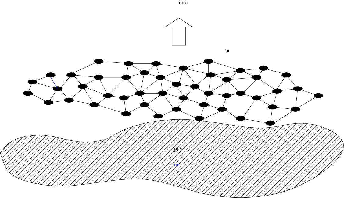
In this paper, we consider ad hoc sensor networks deployed for making statistical inferences about underlying 2-D random fields, and address the above questions in a general 2-D setting. In particular, we investigate the amount of information obtainable from the network and related trade-offs among information, coverage, density and energy in various asymptotic settings, and reveal the fundamental behavior of large scale planar ad hoc sensor networks. We model the signal field as a 2-D Gauss-Markov random field (GMRF), which is suitable for many physical processes, and consider the Kullback-Leibler information (KLI) and mutual information (MI) as our information measures [6, 7]. Our approach for calculating the total obtainable information is based on the large deviations principle (LDP). Under a stationarity assumption, the amount of information from a sensor node becomes independent of sensor location as the network size grows, and the total amount of information is approximately given by the product of the number of sensor nodes and the asymptotic information rate or asymptotic per-node information. (Thus, the units of these quantities is nats/node.) To quantify the information content, we first derive closed-form expressions for the asymptotic per-node KLI and MI for stationary Gaussian fields in a general $d$-dimensional ($d$-D) lattice in the spectral domain, and then apply these results to the 2-D case. We do so by exploiting the spectral structure of $d$-D stationary Gaussian signals and the relationship between the eigenvalues of the block circulant approximation to a block Toeplitz matrix describing the $d$-D correlation structure. However, the general expressions obtained in this way render the investigation of the field correlation and SNR difficult. To address this problem, we adopt the conditional autoregression (CAR) model, which is a generalization of the autoregressive (AR) model of classical time series analysis. We further investigate the properties of the asymptotic per-node KLI and MI as functions of the field correlation and the measurement SNR under the symmetric first order conditional autoregression (SFCAR) model, which captures the 2-D correlation on the plane effectively. In this case, the asymptotic per-node KLI and MI are given explicitly in terms of the SNR and the field correlation. The behavior of the asymptotic per-node KLI and MI as functions of correlation strength is seen to divide into two regions depending on the value of the SNR. At high SNR, uncorrelated observations maximize the per-node information for a given SNR, whereas there is non-zero optimal correlation at low SNR. Interestingly, it is seen that there is a discontinuity in the optimal correlation strength as a function of SNR. In the perfectly correlated case, the asymptotic per-node KLI and MI are zero as expected. As a function of SNR, the asymptotic per-node information increases as $\log\mbox{SNR}$ for a given correlation strength at high SNR. At low SNR, the two information measures show different rates of convergence to zero.

Based on the derived expressions for asymptotic per-node information and their properties under the SFCAR and corresponding correlation function, we then investigate the fundamental behavior of large scale ad hoc sensor networks deployed over correlated random fields for statistical inference. Specifically, we examine the total information [nats] (about the underlying physical process) obtainable from the network and the energy efficiency [nats/J] defined as the ratio of total gathered information to the required energy as the coverage, density and energy vary. We assume that sensors are located on a 2-D lattice and all sensor nodes in the network deliver the measured data to a fusion center in the center of the 2-D lattice via minimum hop routing without in-network data fusion. Under these assumptions, we have the following results on the trade-offs among the information, coverage, density and energy, and the results provide guidelines for the design of sensor networks for statistical inference about many interesting physical processes that can be modelled as 2-D correlated random fields:

• (1)

  When the sensor node density is fixed, the amount of total information increases linearly with respect to (w.r.t.) the coverage area, and the energy efficiency decreases to zero with rate $\Theta\left(\mbox{area}^{-1/2}\right)$ as the coverage area increases. Further, in this case the amount of information per sensor node diminishes to zero as the network size grows with fixed energy per node.

• (2)

  As the sensor spacing $d_{n}$ increases, the per-node information converges to its limit $D$ with rate $D-\sqrt{d_{n}}e^{-\alpha d_{n}}$ for a given diffusion rate $\alpha$. Hence, the per-node information saturates almost exponentially as we increase the sensor spacing.

• (3)

  When the coverage area is fixed and the node density increases, the per-node information is inversely proportional to the node density for any nontrivial diffusion rate. Hence, the total amount of information from a given area is upper bounded unless the random field is spatially white.

• (4)

  As the total energy $E_{t}$ consumed in the network increases, the total information obtainable from the network is given by $\Theta\left(E_{t}^{2/3}\right)$ for fixed node density and increasing coverage, whereas the total information increases only with rate of $O\left(\log E_{t}\right)$ for fixed node density and fixed coverage.

Large deviations analysis of Gaussian processes in Gaussian noise has been considered previously, e.g., [8, 9, 10, 11, 12, 13]. However, most work in this area considers only 1-D signals or time series. A closed-form expression for the asymptotic KLI rate was obtained and its properties were investigated for 1-D hidden Gauss-Markov random processes in [12]. Large deviations analyses were used to examine the issues of optimal sensor density and optimal sampling in a 1-D signal model in [2] and [4]. For a 2-D setting, an error exponent was obtained for the detection of 2-D GMRFs in [14], where the sensors are located randomly and the Markov graph is based on the nearest neighbor dependency enabling a loop-free graph. Our work here focuses on the analysis of the fundamental behavior of 2-D sensor networks deployed for statistical inference via new large deviations results for general $d$-D and 2-D stationary Gaussian random fields and their application to 2-D SFCAR GMRFs, which enable us to investigate the impact of field correlation and measurement SNR on the information and the fundamental behavior of ad hoc sensor networks for statistical inference with preliminary presentation of the work in [15].

We will make use of standard notational conventions. Vectors and matrices are written in boldface with matrices in capitals. All vectors are column vectors. For a matrix ${\bf A}$, ${\bf A}^{T}$ indicates the transpose and ${\bf A}(i,j)$ denotes the $(i,j)$-th element of ${\bf A}$. We reserve ${\bf I}_{m}$ for the identity matrix of size $m$ (the subscript is included only when necessary). For a random vector ${\bf x}$, ${\mathbb{E}}_{j}\{{\bf x}\}$ is the expectation of ${\bf x}$ under probability density $p_{j},~j=0,1$. The notation ${\bf x}\sim{\cal N}(\hbox{\boldmath$\mu$\unboldmath},\hbox{$\bf\Sigma$})$ means that ${\bf x}$ is Gaussian distributed with mean vector $\mu$ and covariance matrix $\bf\Sigma$. For a set ${\cal A}$, $|{\cal A}|$ denotes the cardinality of ${\cal A}$.

The paper is organized as follows. The background and signal model are described in Section II. In Section III, the closed-form expressions for the asymptotic KLI and MI rates are obtained in the spectral domain, and their properties are investigated as functions of the correlation and the SNR under the symmetric first order CAR model. The trade-offs related to ad hoc sensor networks deployed for statistical inference are presented in Section IV, followed by conclusions in Section V.

While the 2-D results are relevant to our analysis of fundamental trade-offs in planar sensor networks, it is of theoretical interest to investigate the statistical properties of stationary Gaussian random fields in general higher dimension. In this section, we first derive closed-form expressions for the asymptotic KLI and MI rates for stationary Gaussian random fields in $d$-D, and then apply the results to the 2-D case. For a stationary $d$-D Gaussian random field $\{Y_{\bf i},~{\bf i}\in{\mathbb{Z}}^{d}\}$, where ${\mathbb{Z}}$ is the set of all integers, the autocovariance function under $p_{1}$ is given by

$$\gamma_{\bf h}={\mathbb{E}}_{1}\{Y_{{\bf i}}Y_{{\bf i}+{\bf h}}\},~~~{\bf h}=(h_{1},h_{2},\cdots,h_{d})\in{\mathbb{Z}}^{d},$$

(21)

and the corresponding Fourier transform (i.e., the power spectral density) and its inverse are given by

$$f_{1}(\hbox{\boldmath$\omega$\unboldmath})=\frac{1}{(2\pi)^{d}}\sum_{{\bf h}\in{\mathbb{Z}}^{d}}\hbox{\boldmath$\gamma$\unboldmath}_{\bf h}e^{-\iota{\bf h}\cdot\hbox{\boldmath$\omega$\unboldmath}},~~~~\hbox{\boldmath$\omega$\unboldmath}=(\omega_{1},\omega_{2},\cdots,\omega_{d})\in[-\pi,\pi)^{d},$$

(22)

and

$$\hbox{\boldmath$\gamma$\unboldmath}_{\bf h}=\int e^{\iota{\bf h}\cdot\hbox{\boldmath$\omega$\unboldmath}}f_{1}(\hbox{\boldmath$\omega$\unboldmath})d\hbox{\boldmath$\omega$\unboldmath},$$

(23)

respectively, where the integration is over $\hbox{\boldmath$\omega$\unboldmath}\in[-\pi,\pi)^{d}$, and ${\bf h}\cdot\hbox{\boldmath$\omega$\unboldmath}$ denotes the inner product between ${\bf h}$ and $\omega$. Note that (21), (22) and (23) are the extensions of (5), (6) and (7), respectively, to $d$-D. The null and alternative distributions arising in the KLI in $d$-D are given by

$$\left\{\begin{array}[]{lcl}p_{0}(Y_{{\bf i}})&:&Y_{{\bf i}}=W_{{\bf i}},~~{\bf i}\in{\cal D}_{n},\\ p_{1}(Y_{{\bf i}})&:&Y_{{\bf i}}={Y}_{{\bf i}}^{(1)},~~{\bf i}\in{\cal D}_{n},\end{array}\right.$$

(24)

where $\{W_{\bf i}\}$ are i.i.d. Gaussian from ${\cal N}(0,\sigma^{2})$, $\{{Y}_{{\bf i}}^{(1)}\}$ is a stationary $d$-D Gaussian random field with spectrum $f_{1}(\hbox{\boldmath$\omega$\unboldmath})$^¶¶ ¶ Note that $\{{Y}_{{\bf i}}^{(1)}\}$ need not be a hidden Markov field., and

$${\cal D}_{n}\stackrel{{\scriptstyle\Delta}}{{=}}[0,1,\cdots,n-1]^{d}.$$

(25)

Based on the previous work [18], we further exploit the relationship between the eigenvalues of block circulant and block Toeplitz matrices representing correlation structure in $d$-D and the i.i.d. null distribution, and obtain the KLI for (24) given by the following theorem.

Proof: See Appendix I.

Applying the $d$-D results to the 2-D hidden GMRF model of (16) and (17), we have the following corollary for 2-D.

Proof: See Appendix I.

Comparing (32) and (33), we note that the asymptotic KLI rate is strictly less than the asymptotic MI rate for any positive signal spectrum, and that the two information measures converge with a fixed offset of -1/2 as the SNR increases without bound since $\frac{\sigma^{2}}{\sigma^{2}+4\pi^{2}f(\omega_{1},\omega_{2})}\rightarrow 0$ in (32) as $\mbox{SNR}\rightarrow\infty$. Hence, the two information measures can be equivalently used at high SNR.

In the previous section, we have derived closed-form expressions for the asymptotic KLI and MI rates for hidden CAR GMRFs with general 2-D spectra defined in (11) in the spectral domain. However, these general spectral expressions render further analysis infeasible. To investigate the impact of the field correlation and the SNR on the information rates, we further adopt the symmetric first order conditional autoregression (SFCAR) model, described by the conditions

$${\mathbb{E}}\{X_{ij}|{\cal X}_{-ij}\}=\frac{\lambda}{\kappa}(X_{i+1,j}+X_{i-1,j}+X_{i,j+1}+X_{i,j-1}),$$

(34)

and

$${\mathbb{E}}^{-1}\{X_{ij}^{2}|{\cal X}_{-ij}\}=\kappa>0,$$

(35)

where $0\leq\lambda\leq\frac{\kappa}{4}$.^∥∥ ∥ This is a sufficient condition to satisfy (12) and (13). Note that the parameters in (8) and (9) for this model are given by $\theta_{00}=\kappa$, $\theta_{1,0}=\theta_{-1,0}=\theta_{0,1}=\theta_{0,-1}=-\lambda$ and all other $\theta_{ij}=0$.

In this model, the correlation is symmetric for each set of four neighboring nodes, as seen in Fig. 3. The SFCAR model is a simple yet meaningful extension of the 1-D first order autoregression (AR) model which has the conditional causal dependency only on the previous sample. Here in the 2-D SFCAR we have the conditional dependency on four neighboring nodes in the four (planar) directions. By Theorem 1 the spectrum of the SFCAR is given by

$$f(\omega_{1},\omega_{2})=\frac{1}{4\pi^{2}\kappa(1-2\zeta\cos\omega_{1}-2\zeta\cos\omega_{2})},$$

(36)

where we define the edge dependence factor $\zeta$ as

$$\zeta\stackrel{{\scriptstyle\Delta}}{{=}}\frac{\lambda}{\kappa},~~~~0\leq\zeta\leq 1/4.$$

(37)

Note that for the range of $0\leq\zeta\leq 1/4$ the 2-D spectrum (36) is always non-negative and the conditions (12) and (13) are satisfied. Note also that $\zeta=0$ corresponds to the i.i.d. case whereas $\zeta=1/4$ corresponds to the perfectly correlated case, i.e., $X_{ij}=X_{i^{\prime}j^{\prime}}$ for all $i,j,i^{\prime},j^{\prime}$. Hence, the correlation strength can be captured in this single quantity $\zeta$ for 2-D SFCAR signals: larger $\zeta$ implies stronger correlation. The power of the SFCAR signal is obtained using the inverse Fourier transform via the relation (6), and is given by [21]

$$P=\gamma_{00}=\frac{2K(4\zeta)}{\pi\kappa},~~~\left(0\leq\zeta\leq\frac{1}{4}\right),$$

(38)

where $K(\cdot)$ is the complete elliptic integral of the first kind. The SNR is given by

$$\mbox{SNR}=\frac{P}{\sigma^{2}}=\frac{2K(4\zeta)}{\pi\kappa\sigma^{2}}.$$

(39)

Using (32), (36) and (39), we now obtain the asymptotic KLI and MI rates in the SCFAR signal case, denoted by ${\mathscr{K}}_{s}$ and ${\mathscr{I}}_{s}$ and given in the following corollary to Corollary 1.

Proof: The result follows upon substitution of (36) and (39) into (32) and (33), respectively.

$\blacksquare$

We first derive how the physical correlation is related to the edge dependence factor $\zeta$ in the 2-D SFCAR model. The edge correlation coefficient $\rho$ is defined as

$$\rho\stackrel{{\scriptstyle\Delta}}{{=}}\frac{\gamma_{01}}{\gamma_{00}}=\frac{\gamma_{10}}{\gamma_{00}},~~(0\leq\rho\leq 1),$$

(53)

due to the spatial symmetry, where $\gamma_{ij}={\mathbb{E}}\{X_{00}X_{ij}\}$. $\rho$ represents the correlation strength between the signal samples of two adjacent sensor nodes connected by the Markov dependence graph defined by the SFCAR model. The edge correlation coefficient $\rho$ is obtained using the following relationship [21]:

$$\kappa\gamma_{00}=1+4\zeta\kappa\gamma_{01}~~~\Rightarrow~~~\gamma_{01}=\frac{\kappa\gamma_{00}-1}{4\kappa\zeta},$$

(54)

and by substituting (38) and (54) into (53), we have

$$\rho=\frac{(2/\pi)K(4\zeta)-1}{(2/\pi)(4\zeta)K(4\zeta)}=:g^{-1}(\zeta).$$

(55)

Note that the correlation coefficient $\rho$ is not dependent on the power factor $\kappa$ in (35), as expected, even though $\gamma_{00}$ and $\gamma_{01}$ are. Note that function $g^{-1}:\zeta\rightarrow\rho$ is a continuous and differentiable $C^{1}$ function on the domain $0\leq\zeta\leq 1/4$ due to the continuous differentiability of $K(x)$ for $0\leq x<1$, and $g^{-1}(1)=\lim_{x\rightarrow 1}\frac{(2/\pi)K(x)-1}{(2/\pi)xK(x)}=1$ by $K(1)=\infty$. Note also that $g^{-1}(0)=0$ since $K(0)=\pi/2$. Thus, the inverse mapping $g:\rho\rightarrow\zeta$ from the edge correlation factor $\rho$ to the edge dependence factor $\zeta$, which maps zero and one to zero and 1/4, respectively, behaves as shown in Fig. 7 (a).

Now we consider the correlation coefficient $\rho$ as a function of the sensor spacing $d_{n}$. In general, the correlation function $h:d_{n}\rightarrow\rho$ is a positive and monotonically decreasing function of $d_{n}$ with $h(0)=1$ and $h(\infty)=0$. It is well known that for the 1-D first order AR signal a corresponding underlying (continuous-index) physical model is given by the Ornstein-Uhlenbeck process

$$\frac{ds(x)}{dx}=-As(x)+Bu(x),$$

(56)

and its discrete-time equivalent is given by

$$\left\{\begin{array}[]{ccl}s_{i+1}&=&as_{i}+u_{i},\\ a&=&{\mathbb{E}}\{s_{i}s_{i-1}\}/{\mathbb{E}}\{s_{i}^{2}\}=e^{-Ad_{n}},\end{array}\right.$$

(57)

where $A\geq 0$,  $B\in{\mathbb{R}}$,  $s_{i}=s(id_{n})$, and the input processes $u(x)$ and $u_{i}$ are zero-mean white Gaussian processes. Here, $d_{n}$ is the spacing between two adjacent signal samples. For the 2-D SFCAR signal, however, the same stochastic differential equation is not applicable. Note that the dependence in the signal in (56) and (57) is only on the past in 1-D space, whereas the signal (34) has symmetric dependence in all four direction in the plane. The SFCAR signal is given by the solution of a second-order difference equation

$$X_{ij}=\zeta(X_{i+1,j}+X_{i-1,j}+X_{i,j+1}+X_{i,j-1})+\epsilon_{ij},$$

(58)

and the corresponding continuous-index physical model is given by the stochastic Laplace equation [23].

$$\left[\left(\frac{\partial}{\partial x}\right)^{2}+\left(\frac{\partial}{\partial y}\right)^{2}-\alpha^{2}\right]X(x,y)=\epsilon(x,y),$$

(59)

where $\alpha~(\geq 0)$ is the physical diffusion rate, and $\epsilon_{ij}$ and $\epsilon(x,y)$ are 2-D white zero-mean Gaussian perturbations. Note that the solution of (59) is circularly symmetric, i.e., it depends only on $r=\sqrt{x^{2}+y^{2}}$, and samples of the solution $X(x,y)$ of (59) on lattice ${\cal I}_{n}$ do not form a discrete-index SFCAR GMRF. However, (59) is still the continuous-index counterpart of (58), and we use its correlation function for the SFCAR model. The correlation function corresponding to (59) is given by [23]

$$\rho=h(d_{n})=\alpha d_{n}K_{1}(\alpha d_{n}),$$

(60)

where $K_{1}(\cdot)$ is the modified Bessel function of the second kind. Fig. 7 (b) shows the correlation function w.r.t. $d_{n}$ for $\alpha=1$. The asymptotic behavior of $K_{1}(x)$ is given by

$$\left\{\begin{array}[]{cccl}K_{1}(x)&\rightarrow&\sqrt{\frac{\pi}{2x}}e^{-x}&\mbox{as}~x\rightarrow\infty,\\ K_{1}(x)&\rightarrow&\frac{1}{x}&\mbox{as}~x\rightarrow 0.\\ \end{array}\right.$$

(61)

The correlation function (60) can be regarded as the representative correlation in 2-D, similar to the exponential correlation function $e^{-Ad_{n}}$ in 1-D. Both functions decrease monotonically w.r.t. $d_{n}$. However, the 2-D correlation function is flat at $d_{n}=0$ [23], i.e.,

$$\left(\frac{d\rho}{dd_{n}}\right)_{d_{n}=0}=0,$$

(62)

and it decays with rate $\sqrt{d_{n}}e^{-\alpha d_{n}}$ as $d_{n}\rightarrow\infty$. Note that the 2-D correlation function has $\sqrt{d_{n}}$ in front of the exponential decay as $d_{n}\rightarrow\infty$. However, this polynomial term is not significant and the exponential decay is dominant for large $d_{n}$. Thus, we have $\zeta=g(h(d_{n})),$ and for given physical parameters (with a slight abuse of notation),

$${\mathscr{K}}_{s}(\mbox{SNR},\zeta)={\mathscr{K}}_{s}(\mbox{SNR},g(h(d_{n})))={\mathscr{K}}_{s}(\mbox{SNR},d_{n}),$$

and

$${\mathscr{I}}_{s}(\mbox{SNR},\zeta)={\mathscr{I}}_{s}(\mbox{SNR},g(h(d_{n})))={\mathscr{I}}_{s}(\mbox{SNR},d_{n}).$$

We will use the arguments SNR, $\zeta$ and $d_{n}$ for ${\mathscr{K}}_{s}$ and ${\mathscr{I}}_{s}$ properly as needed for exposition.

References

- [1] D. Estrin, D. Culler, K. Pister and G. Sukhatme, “Connecting the physical world with pervasive networks,” IEEE Pervasive Computing, vol. 1, no. 1, pp. 59-69, Jan.-Mar. 2002.
- [2] J.-F. Chamberland and V. V. Veeravalli, “How dense should a sensor network be for detection with correlated observations?,” IEEE Transactions on Information Theory, vol. 52, no. 11, pp. 5099 - 5106, Nov. 2006.
- [3] M. Dong, L. Tong and B. M. Sadler, “Impact of data retrieval pattern on homogeneous signal field reconstruction in dense sensor networks,” IEEE Transactions on Signal Processing, vol. 54, no. 11, pp. 4352 - 4364, Nov. 2006.
- [4] Y. Sung, X. Zhang, L. Tong and H. V. Poor, “Sensor configuration and activation for field detection in large sensor arrays,” IEEE Transactions on Signal Processing, vol. 56, no. 2, pp. 1354 - 1365, Feb. 2008.
- [5] L. S. Pillutla and V. Krishnamurthy, “Mutual information and energy tradeoff in correlated wireless sensor networks,” in Proc. 2008 IEEE International Conference on Communications (ICC), Beiging, China, May 2008.
- [6] F. Liese and I. Vajda, “On divergence and informations in statistics and information theory,” IEEE Transactions on Information Theory, vol. 52, no. 10, pp. 4394 - 4412, Oct. 2006.
- [7] S. Kullback, Information Theory and Statistics. Dover Publications, Inc., Mineola, NY, 1997.
- [8] M. D. Donsker and S. R. S. Varadhan, “Large deviations for stationary Gaussian process,” Communications in Mathematical Physics, vol. 97, pp. 187 - 210, 1985.
- [9] G. R. Benitz and J. A. Bucklew, “Large deviation rate calculations for nonlinear detectors in Gaussian noise,” IEEE Transactions on Information Theory, vol. 36, no. 2, pp. 358 - 371, Mar. 1990.
- [10] W. Bryc and A. Dembo, “Large deviations for quadratic functionals of Gaussian processes,” Journal of Theoretical Probability, vol. 10, no. 2, pp. 307 - 332, 1997.
- [11] B. Bercu, F. Gamboa and A. Rouault, “Large deviations for quadratic forms of stationary Gaussian processes,” Stochastic Processes and Their Applications, vol. 71, pp. 75 - 90, 1997.
- [12] Y. Sung, L. Tong and H. V. Poor, “Neyman-Pearson detection of Gauss-Markov signals in noise: Closed-form error exponent and properties,” IEEE Transactions on Information Theory, vol. 52, no. 4, pp. 1354 - 1365, Apr. 2006.
- [13] A. S. Leong, S. Dey and J. S. Evans, “Error exponents for Neyman-Pearson detection of Markov chains in noise,” IEEE Transactions on Signal Processing, vol. 55, no. 10, pp. 5097 - 5103, Oct. 2007.
- [14] A. Anandkumar, L. Tong and A. Swami, “Detection of Gauss-Markov random field on nearest-neighbor graph,” in Proc. 2007 IEEE International Conference on Acoustics, Speech, and Signal Processing (ICASSP’07), Honolulu, HI, Apr. 2007. Oct. 2007.
- [15] Y. Sung, H. V. Poor and H. Yu, “Information, energy and density for ad hoc sensor networks over correlated random fields: Large deviations analysis,” in Proc. 2008 International Symposium on Information Theory (ISIT), Toronto, Ontario, Canada, Jul. 2008.
- [16] H. Rue and L. Held, Gaussian Markov Random Fields: Theory and Applicatons. Chapman & Hall/CRC, New York, 2005.
- [17] R. R. Bahadur, S. L. Zabell and J. C. Gupta, “Large deviations, tests, and estimates,” in I. M. Chakravarti, ed., Asymptotic Theory of Statistical Tests and Estimation: In Honor of Wassily Hoeffding, Academic Press, New York, 1980.
- [18] J. T. Kent and K. V. Mardia, “Spectral and circulant approximations to the likelihood for stationary Gaussian random fields,” Journal of Statistical Planning and Inference, vol. 502, no. 3, pp. 379 - 394, 1996.
- [19] R. R. Bahadur, “Some Limit Theorems in Statistics,” in Conference Board of the Mathematical Sciences Regional Conferences Series in Applied Mathematics, SIAM, no. 4, Philadelphia, PA, 1971.
- [20] T. Cover and J. Thomas, Elements of Information Theory. John Wiley & Sons, Inc., New York, 1991.
- [21] J. Besag, “On a system of two-dimensional recurrence equations,” Journal of the Royal Statistical Society. Series B, vol. 43, no. 3, pp. 302 - 309, 1981.
- [22] A. Erdélyi, Higher Transcendental Functions, Vol. II. McGraw-Hill, New York, 1953.
- [23] P. Whittle, “On stationary processes in the plane,” Biometrika, vol. 41, no. 3, pp. 434 - 449, Dec. 1954.
- [24] I. Vajda, Theory of Statistical Inference and Information. Kluwer Academic Publishers, Dordrecht, 1989.
- [25] P. J. Brockwell and R. A. Davis, Time Series: Theory and Methods. 2nd Edition, Springer, New York, 1991.
- [26] E. J. Hannon, “The asymptotic theory of linear time-series models,” Journal of Applied Probability, vol. 10, no. 1, pp. 130 - 145, Mar. 1973.
- [27] X. Guyon, Random Fields on a Network: Modeling, Statistics and Applications. Springer-Verlag, New York, 1995.
- [28] I. Gohberg, S. Goldberg and M. A. Kaashoek, Basic Classes of Linear Operators. Birkhäuser, Basel, Switzerland, 2004.
- [29] R. J. Martin, “A note on the asymptotic eigenvalues and eigenvectors of the dispersion matrix of a second-order stationary process on a -dimensional lattice,” Journal of Applied Probability, vol. 23, no. 2, pp. 529 - 535, Jun. 1986.
- [30] P. J. Davis, Circulant Matrices. Chelsea Publishing, New York, 1994.