跳到论文正文
W Papers独立论文阅读器 arXiv:0903.1397 论文正文 计算阅读时间 · 0%
引用这篇论文根据当前论文元数据生成,正式投稿前建议核对。


License: arXiv.org perpetual non-exclusive license
arXiv:0903.1397v1 [math.DS] 08 Mar 2009

Platonic Polyhedra, Topological Constraints and Periodic Solutions of the Classical NN-Body Problem

G. Fusco Affiliation: Dip. di Matematica Pura ed Applicata, Università di L’Aquila    G. F. Gronchi Affiliation: Dip. di Matematica, Università di Pisa    P. Negrini Affiliation: Dip. di Matematica, Università di Roma ‘La Sapienza’
Received: date / Revised version: date
Abstract

We prove the existence of a number of smooth periodic motions u∗u_{*} of the classical Newtonian NN–body problem which, up to a relabeling of the NN particles, are invariant under the rotation group ℛ{\cal R} of one of the five Platonic polyhedra. The number NN coincides with the order |ℛ||{\cal R}| of ℛ{\cal R} and the particles have all the same mass. Our approach is variational and u∗u_{*} is a minimizer of the Lagrangean action 𝒜{\mathcal{A}} on a suitable subset 𝒦{\mathcal{K}} of the H1H^{1} TT–periodic maps u:ℝ→ℝ3​Nu:{\mathbb{R}}\to{\mathbb{R}}^{3N}. The set 𝒦{\mathcal{K}} is a cone and is determined by imposing to uu both topological and symmetry constraints which are defined in terms of the rotation group ℛ{\cal R}. There exist infinitely many such cones 𝒦{\mathcal{K}}, all with the property that 𝒜|𝒦{\mathcal{A}}|_{{\mathcal{K}}} is coercive. For a certain number of them, using level estimates and local deformations, we show that minimizers are free of collisions and therefore classical solutions of the NN–body problem with a rich geometric–kinematic structure.

Propositum est mihi, Lector, hoc libello demonstrare, quod Creator Optimus Maximus, in creatione mundi huius mobilis, et dispositione coelorum, ad illa quinque regularia corpora, inde a Pythagora et Platone, ad nos utque, celebratissima respexerit, atque ad illorum naturam coelorum numerum, proportiones, et motuum rationem accommodaverit. (J. Kepler, Myst. Cosm. [20])

List of symbols

symbol meaning
𝔗{\mathfrak{T}}, ℭ{\mathfrak{C}}, 𝔒{\mathfrak{O}}, 𝔇{\mathfrak{D}}, ℑ{\mathfrak{I}} the five Platonic polyhedra
𝒯,𝒪,ℐ{\cal T},{\cal O},{\cal I} symmetry groups of rotations of the Platonic polyhedra
𝒬𝒯,𝒬𝒪,𝒬ℐ{\cal Q}_{\cal T},{\cal Q}_{\cal O},{\cal Q}_{\cal I} Archimedean polyhedra, Section 4.1
𝒳\mathcal{X} configuration space
𝔖\mathfrak{S} loops with collisions
Γ\Gamma set of the axes of rotation of the group ℛ∈{𝒯,𝒪,ℐ}{\cal R}\in\{{\cal T},{\cal O},{\cal I}\}
ℛ~\tilde{\cal R} reflection group associated to ℛ{\cal R}
uu generic element of HT1​(ℝ,R3​N)H^{1}_{T}({\mathbb{R}},R^{3N}) and
𝖯1\mathsf{P}_{1} generating particle
τ1\tau_{1} trajectory of the generating particle
u1u_{1} generating loop for uu
uˇ1\check{u}_{1}, u^1\hat{u}_{1} variations of u1u_{1}
u∗u_{*}, u∗,1u_{*,1} minimizer and related generating loop
Λ(𝖺)\Lambda^{{\sf(a)}}, Λ0(𝖺)\Lambda_{0}^{\sf(a)} loop spaces
Λ0(𝖺)/∼\Lambda_{0}^{\sf(a)}\hskip-4.26773pt/\hskip-4.26773pt\sim space of equivalence classes of loops in Λ0(𝖺)\Lambda_{0}^{\sf(a)}
𝒦{\mathcal{K}}, 𝒦iP{\mathcal{K}^{P}_{i}}, 𝒦~ν\tilde{{\mathcal{K}}}^{\nu} cones of loops
𝖲2\mathsf{S}^{2} unit sphere in ℝ3{\mathbb{R}}^{3}
𝖾j\mathsf{e}_{j} direction vector of the axis ξj,j=1,2,3\xi_{j},j=1,2,3
ℕ{\mathbb{N}} natural numbers excluding 0
u1(σ,n){\rm u}^{(\sigma,n)}_{1} map associated to a periodic sequence (σ,n)(\sigma,n) of domains DkD_{k}, see (4.3)
v1(ν,n){\rm v}_{1}^{(\nu,n)} map associated to a periodic sequence (ν,n)(\nu,n) of vertexes of 𝒬ℛ{\cal Q}_{\cal R}, see (4.14)
D{\rm D} fundamental domain
S1{\rm S}_{1}, S2{\rm S}_{2}, S3{\rm S}_{3} faces of D{\rm D}
DkD_{k} domains obtained by applying the elements of ℛ~\tilde{\cal R} to D{\rm D}
SkS_{k}, SkS^{k} faces of DkD_{k}
RSR_{S} reflection with respect to the plane of the face SS
R↦RSR\mapsto R^{S} bijection defined in ℛ∖{I}{\cal R}\setminus\{I\} for a given SS, cfr. (4.17)

1 Introduction

In the last few years many interesting periodic motions of the classical Newtonian NN–body problem have been discovered as minimizers of the Action functional

𝒜:ΛG→ℝ∪{+∞},{\mathcal{A}}:\Lambda_{G}\to{\mathbb{R}}\cup\{+\infty\}\,,
𝒜⁡(u)=∫0T(12​∑h=1Nmh​|u˙h|2+∑1≤h<k≤Nmh​mk|uh−uk|)​𝑑t{\mathcal{A}}(u)=\int_{0}^{T}\Bigl(\frac{1}{2}\sum_{h=1}^{N}m_{h}|\dot{u}_{h}|^{2}+\sum_{1\leq h<k\leq N}\frac{m_{h}\,m_{k}}{|u_{h}-u_{k}|}\Bigr)\,dt (1.1)

on loop spaces ΛG⊂HT1​(ℝ,𝒳)\Lambda_{G}\subset H^{1}_{T}({\mathbb{R}},\mathcal{X}), of TT–periodic motions, equivariant with respect to the action of a suitably chosen group GG [14],[5]. We denote by u=(u1,…,uN):ℝ→𝒳u=(u_{1},\dots,u_{N}):{\mathbb{R}}\to\mathcal{X} a typical element of ΛG\Lambda_{G}, by uh:ℝ→ℝ3u_{h}:{\mathbb{R}}\to{\mathbb{R}}^{3} the motion of the mass mhm_{h} and by 𝒳⊂ℝ3​N\mathcal{X}\subset{\mathbb{R}}^{3N} the configuration space

𝒳={x=(x1,…,xN)∈ℝ3​N:∑h=1Nmh​xh=0}.\mathcal{X}=\Bigl\{x=(x_{1},\ldots,x_{N})\in{\mathbb{R}}^{3N}:\sum_{h=1}^{N}m_{h}x_{h}=0\Bigr\}\ .

HT1​(ℝ,𝒳)H^{1}_{T}({\mathbb{R}},\mathcal{X}) denotes the Sobolev space of L2L^{2} TT–periodic maps u:ℝ→𝒳u:{\mathbb{R}}\to\mathcal{X} with L2L^{2} first derivative.

The interest in this classical problem was revived by the discovery of the now famous Eight [22], [3]: the rather surprising fact that three equal masses can move periodically one after the other with a time shift of T/3T/3 on the same fixed planar trajectory which has the shape of a symmetric eight. Another remarkable motion is the Hip–Hop [8], [12] where four equal masses, at intervals of T/2T/2, coincide alternatively with the vertexes of two tetrahedra, each one symmetric of the other with respect to the center of mass.

The lack of coercivity of the action functional on the whole set HT1​(ℝ,𝒳)H^{1}_{T}({\mathbb{R}},\mathcal{X}) of TT–periodic motions and the fact that, on the basis of Sundman’s estimates [31], [26], collisions give a bounded contribution to the action are the main mathematical obstructions in the search for TT–periodic motions of the NN–body problem as minimizers of the action. One of the main results of the research effort developed in the last ten years is a quite systematic way to deal with these obstructions. A basic observation concerning the problem of coercivity is that the action functional (1.1) is coercive when restricted to a loop space ΛG\Lambda_{G} of motions that possess suitable symmetries. The idea to impose symmetries to obtain coercivity was introduced in [11] and used in [7], and it is considered in a general abstract context in [14], where also a necessary and sufficient condition for coercivity is given.

The original motivation for our work was aesthetical: we wondered about the existence of new periodic motions which we could compare in perfection and beauty with the Eight, the Hip–Hop and the other interesting motions that have been recently discovered, see [27], [2], [28].

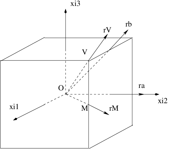
Let PP be one of the five Platonic polyhedra, that is P∈{𝔗P\in\{{\mathfrak{T}}, ℭ{\mathfrak{C}}, 𝔒{\mathfrak{O}}, 𝔇{\mathfrak{D}}, ℑ}{\mathfrak{I}}\} where 𝔗,ℭ,𝔒,𝔇,ℑ{\mathfrak{T}},{\mathfrak{C}},{\mathfrak{O}},{\mathfrak{D}},{\mathfrak{I}} stand for Tetrahedron, Cube, Octahedron, Dodecahedron and Icosahedron. Let 𝒯,𝒪,ℐ{\cal T},{\cal O},{\cal I} be the groups of rotations of 𝔗{\mathfrak{T}}, of ℭ{\mathfrak{C}} and 𝔒{\mathfrak{O}}, of 𝔇{\mathfrak{D}} and ℑ{\mathfrak{I}} respectively, and denote by ℛ∈{𝒯,𝒪,ℐ}{\cal R}\in\{{\cal T},{\cal O},{\cal I}\} the group of rotations of PP. Let K=4,6,8,12,20K=4,6,8,12,20 be the number of the faces of PP and H=3,4,3,5,3H=3,4,3,5,3 the number of the vertexes of each face of PP. Let FF be one of the faces of PP, LL one of the sides of FF and MM the middle point of LL. Consider a right–handed orthogonal frame O​ξ1​ξ2​ξ3O\xi_{1}\xi_{2}\xi_{3}, with the origin in the center of PP, the axis ξ1\xi_{1} oriented from OO to the center of FF and the axes ξ2,ξ3\xi_{2},\xi_{3} such that MM lies in the half–plane {ξ3=0,ξ2>0}\{\xi_{3}=0,\xi_{2}>0\}. We let VV be the vertex of LL in the half–space ξ3>0\xi_{3}>0 (see Figure 3). We denote by 𝖾j\mathsf{e}_{j} the direction vector of ξj,j=1,2,3\xi_{j},j=1,2,3. The question that was at the origin of the present work is the following:

(Q) Does it exist a TT–periodic motion of the classical Newtonian NN–body problem with N=H​K=12,24,60N=HK=12,24,60 equal masses that satisfies conditions (a), (b), (c) below?

  • (a)

    If u1:ℝ→ℝ3u_{1}:{\mathbb{R}}\to{\mathbb{R}}^{3}, u1​(t+T)=u1​(t)​∀t∈ℝu_{1}(t+T)=u_{1}(t)\ \forall t\in{\mathbb{R}}, is the motion of one of the NN particles, called the generating particle, the motion of the NN particles is determined by a bijection:

    {2,…,N}∋j→Rj∈ℛ∖{I}:uj=Rj​u1.\{2,\dots,N\}\ni j\to R_{j}\in{\cal R}\setminus\{I\}:u_{j}=R_{j}u_{1}\ . (1.2)
  • (b)

    Associated to each face of PP there are HH particles that move one after the other on the same trajectory with a time shift of T/HT/H.

  • (c)

    The motion of the generating particle satisfies

    u1​(t)=S3​u1​(−t)∀t∈ℝ,u_{1}(t)=S_{3}u_{1}(-t)\quad\quad\forall t\in{\mathbb{R}}\,,

    where S3S_{3} is the reflection with respect to the plane ξ3=0\xi_{3}=0.

We remark that (a), (b), (c) imply in particular that the trajectory

τ1={x∈ℝ3:∃t​ with ​x=u1​(t)}\tau_{1}=\{x\in{\mathbb{R}}^{3}:\exists\,t\mbox{ with }x=u_{1}(t)\}

has all the symmetries of FF.

OPENa)a)Refer to caption      OPENb)b)Refer to caption

Figure 1: Loops in the space ΛP\Lambda^{P} for P=ℭP={\mathfrak{C}}.

We denote by ΛP⊂HT1​(ℝ,𝒳)\Lambda^{P}\subset H^{1}_{T}({\mathbb{R}},\mathcal{X}) the subset of TT–periodic maps that satisfy conditions (a), (b), (c). Figure 1 visualizes possible structures of motions that satisfy (a), (b), (c) for the case P=ℭP={\mathfrak{C}}. One checks immediately that the action functional (with mj=1,j=1​…​Nm_{j}=1,\,j=1\ldots N)

𝒜⁡(u)=N2​∫0T(|u˙1|2+∑Rj∈ℛ∖{I}1|(Rj−I)​u1|)​𝑑t{\mathcal{A}}(u)=\frac{N}{2}\int_{0}^{T}\biggl(|\dot{u}_{1}|^{2}+\sum_{R_{j}\in{\cal R}\setminus\{I\}}\frac{1}{|(R_{j}-I)u_{1}|}\biggr)\,dt (1.3)

is not coercive on the loop space ΛP\Lambda^{P}. Indeed, if we set u1λ=u1+λ​𝖾1u_{1}^{\lambda}=u_{1}+\lambda\mathsf{e}_{1}, λ>0\lambda>0, 𝖾1=(1,0,0)\mathsf{e}_{1}=(1,0,0), we have

𝒜⁡(u)−𝒜⁡(uλ)=N2​∫0T∑Rj∈ℛ∖{I}(1|(Rj−I)​u1|−1|(Rj−I)​u1+λ⁡(Rj−I)​𝖾1|)​𝑑t{\mathcal{A}}(u)-{\mathcal{A}}(u^{\lambda})=\frac{N}{2}\int_{0}^{T}\sum_{R_{j}\in{\cal R}\setminus\{I\}}\left(\frac{1}{|(R_{j}-I)u_{1}|}-\frac{1}{|(R_{j}-I)u_{1}+\lambda(R_{j}-I)\mathsf{e}_{1}|}\right)\,dt

and therefore 𝒜⁡(u)−𝒜⁡(uλ)>0{\mathcal{A}}(u)-{\mathcal{A}}(u^{\lambda})>0 for λ\lambda large enough. This is also a consequence of the abstract coercivity condition formulated in [14]. In [14] a motion u:ℝ→𝒳u:{\mathbb{R}}\to\mathcal{X} is said to be equivariant with respect to the action of a finite group GG if

ρ⁡(g)​uσ​(g−1)​(i)​(t)=ui​(τ⁡(g)​(t))∀g∈G,∀t∈ℝ,∀i∈{1​…​N}.\rho(g)\;u_{\sigma(g^{-1})(i)}(t)=u_{i}(\tau(g)(t))\qquad\forall\,g\in G,\ \forall\,t\in{\mathbb{R}},\ \forall\,i\in\{1\dots N\}\ . (1.4)

Here ρ:G→O⁡(3)\rho:G\to O(3), τ:G→O⁡(2)\tau:G\to O(2) are orthogonal representations of GG and σ:G→SN\sigma:G\to S_{N} is a homomorphism of GG to SNS_{N}, the group of permutations of {1​…​N}\{1\dots N\}.11 1 If the masses of the NN particles are not all equal it is required that σ⁡(g)​(i)=j⇒mi=mj\sigma(g)(i)=j\Rightarrow m_{i}=m_{j}. If we let ΛG⊂HT1​(ℝ,𝒳)\Lambda_{G}\subset H^{1}_{T}({\mathbb{R}},\mathcal{X}) be the set of loops that fulfill the equivariance condition (1.4), then the coercivity condition formulated and proven in [14] is the following:

Theorem 1.1.

The action functional 𝒜{\mathcal{A}} is coercive on ΛG\Lambda_{G} if and only if

𝒳G={0}\mathcal{X}^{G}=\{0\} (1.5)

where 𝒳G⊂ℝ3​N\mathcal{X}^{G}\subset{\mathbb{R}}^{3N} is the subset of the configuration space invariant under GG, that is

𝒳G={x∈𝒳:ρ(g)xσ​(g−1)​(i)=xi,∀g∈G,∀i∈{1…N}}.\mathcal{X}^{G}=\bigl\{x\in\mathcal{X}:\rho(g)x_{\sigma(g^{-1})(i)}=x_{i},\forall\,g\in G,\ \forall\,i\in\{1\dots N\}\bigr\}\ .

For the loop space ΛG=ΛP\Lambda_{G}=\Lambda^{P}, defined by (a), (b), (c), condition (1.5) is not satisfied. Indeed the nonzero vector

x=(x1,…,xN),x1=𝖾1,xj=Rj𝖾1,j=2,…,Nx=(x_{1},\ldots,x_{N}),\qquad x_{1}=\mathsf{e}_{1}\,,x_{j}=R_{j}\mathsf{e}_{1},\ j=2,\ldots,N

belongs to 𝒳G\mathcal{X}^{G}.

The fact that for ΛG=ΛP\Lambda_{G}=\Lambda^{P} condition (1.5) is violated does not exclude a priori a positive answer to question (Q). Actually, in spite of the non–coercivity of 𝒜{\mathcal{A}} on ΛP\Lambda^{P}, motions defined by (a), (b), (c) may correspond to local minimizers, that may exist even though (1.5) is not satisfied. We also remark that for a loop u⁡(t)u(t) that satisfies (1.5) we necessarily have

u¯=1T​∫0Tu⁡(t)​𝑑t=0.\bar{u}=\frac{1}{T}\int_{0}^{T}u(t)\,dt=0\ . (1.6)

This follows from (1.4), that implies

∫0Tui​(t)​𝑑t=∫0Tui​(τ⁡(g)​(t))​𝑑t=ρ⁡(g)​∫0Tuσ​(g−1)​(i)​(t)​𝑑t,\int_{0}^{T}u_{i}(t)\,dt=\int_{0}^{T}u_{i}(\tau(g)(t))\,dt=\rho(g)\int_{0}^{T}u_{\sigma(g^{-1})(i)}(t)\,dt\,,

which is equivalent to u¯i=ρ⁡(g)​u¯σ​(g−1)​(i)\bar{u}_{i}=\rho(g)\bar{u}_{\sigma(g^{-1})(i)}. Clearly (1.6) poses strong geometric restrictions on the motion and we may expect that many complex and interesting motions with a rich geometric–kinematic structure correspond to local minimizers that, as the loops defined by (a), (b), (c), do not need to satisfy condition (1.6). Is it possible to detect some of these local minimizers? Let 𝔖⊂ΛG\mathfrak{S}\subset\Lambda_{G} be the subset of the loops that present collisions:

𝔖={u∈ΛG:∃tc∈ℝ,h≠k∈{1…N}:uh(tc)=uk(tc)}.\mathfrak{S}=\{u\in\Lambda_{G}:\exists\,t_{c}\in{\mathbb{R}},h\neq k\in\{1\dots N\}:u_{h}(t_{c})=u_{k}(t_{c})\}\ .

This is a well defined subset of ΛG\Lambda_{G}, closed in the C0C^{0} topology. We focus on open cones 𝒦⊂ΛG{\mathcal{K}}\subset\Lambda_{G} with the property

∂𝒦⊂𝔖\partial{\mathcal{K}}\subset\mathfrak{S} (1.7)

where ∂𝒦\partial{\mathcal{K}} is the C0C^{0} boundary of 𝒦{\mathcal{K}}. The idea is that 𝒜{\mathcal{A}} can be coercive on 𝒦{\mathcal{K}} even though (1.5) is not satisfied; if we are able to prove that a minimizer u∗u_{*} of 𝒜|𝒦¯{\mathcal{A}}|_{\overline{\mathcal{K}}} exists and is collision free, then automatically we have u∗∈𝒦u_{*}\in{\mathcal{K}} and therefore a genuine solution of the NN–body problem. In the following we discuss non–trivial situations where the above ideas can be successfully applied. Indeed we show the existence of new TT–periodic solutions of the classical NN–body problem with a rather rich and complex structure. In particular we give a positive answer to question (Q). These results are precisely stated in Theorems 2.3, 3.3, 4.9 below.

We remark that restricting the action to a cone 𝒦⊂ΛG{\mathcal{K}}\subset\Lambda_{G} that satisfies (1.7) corresponds to the introduction of topological constraints beside the symmetry constraints imposed by the equivariance condition (1.4). The idea to obtain coercivity by introducing topological constraints, that restrict the action to subsets 𝒦{\mathcal{K}} satisfying condition (1.7), goes back to Poincaré [25] and has been exploited in [18], [29], [28]. In the proof that minimizers u∗u_{*} of 𝒜|𝒦¯{\mathcal{A}}|_{\overline{\mathcal{K}}}, for the considered cones 𝒦{\mathcal{K}}, are free of collisions we take advantage of ideas of various authors [21], [5], [30]. Moreover we need to overcome the extra difficulty of dealing with a topological constraint, that does not allow general perturbations of u∗∈∂𝒦u_{*}\in\partial{\mathcal{K}}, but only those that move u∗u_{*} inside 𝒦{\mathcal{K}}. For this reason Marchal’s idea of averaging the action on a sphere or the average on a suitable circle, leading to the definition of the rotating circle property in [14], can not be applied in our context. The paper is organized as follows: in Sections 2, 3 and 4 we define different kinds of cones 𝒦{\mathcal{K}} that satisfy (1.7), and we prove the coercivity of 𝒜|𝒦{\mathcal{A}}|_{{\mathcal{K}}}. In Section 5 we prove Theorems 2.3, 3.3, 4.9 by showing that, for certain cones 𝒦{\mathcal{K}}, minimizers u∗∈𝒦u_{*}\in{\mathcal{K}} are collision free. In Section 5.1 we exclude total collisions by means of level estimates. In Section 5.2 we exclude partial collisions via local perturbations. In Section 6 we present conjectures and numerical experiments, and prove the existence of TT–periodic motions that violate (1.6).

2 An example of cone 𝒦{\mathcal{K}}

We consider the set of TT-periodic loops of N=4N=4 unit masses that satisfy

{u1​(t)=S3​u1​(−t)u1​(T4+t)=S2​u1​(T4−t)\left\{\begin{array}[]{l}u_{1}(t)=S_{3}u_{1}(-t)\cr u_{1}(\frac{T}{4}+t)=S_{2}u_{1}(\frac{T}{4}-t)\cr\end{array}\right. (2.1)
{u2​(t)=R3​u1​(t)u3​(t)=R1​u1​(t)u4​(t)=R2​u1​(t)\left\{\begin{array}[]{l}u_{2}(t)=R_{3}u_{1}(t)\cr u_{3}(t)=R_{1}u_{1}(t)\cr u_{4}(t)=R_{2}u_{1}(t)\cr\end{array}\right.\hskip 42.67912pt (2.2)

where SjS_{j} is the reflection with respect to the plane ξj=0\xi_{j}=0, j=1,2,3j=1,2,3, and RjR_{j} is the rotation of π\pi around the axis ξj\xi_{j}, j=1,2,3j=1,2,3 (cfr. Figure 2). The loop space defined by (2.1) and (2.2) does not satisfy condition (1.5). Indeed the vector x∈𝒳⊂ℝ12x\in\mathcal{X}\subset{\mathbb{R}}^{12} defined by

x1=x3=𝖾1,x2=x4=−𝖾1x_{1}=x_{3}=\mathsf{e}_{1}\,,\quad x_{2}=x_{4}=-\mathsf{e}_{1}

is in 𝒳G\mathcal{X}^{G} and therefore, by Theorem 1.1, 𝒜\mathcal{A} is not coercive on ΛG\Lambda_{G} as one can also directly verify. Following the approach outlined above, we regain coercivity by restricting the set of allowed loops to the cone

𝒦4={u∈ΛG:u11​(0)​u11​(T/4)<0}.{\mathcal{K}_{4}}=\{u\in\Lambda_{G}:u_{11}(0)u_{11}(T/4)<0\}\ . (2.3)

We denote with (u11,u12,u13)(u_{11},u_{12},u_{13}) the components of u1u_{1}.

Proposition 2.1.

The cone 𝒦4{\mathcal{K}_{4}} satisfies condition (1.7) and 𝒜|𝒦4\mathcal{A}|_{{\mathcal{K}_{4}}} is coercive.

Proof 2.2.

From (2.3) it follows [u11​(0)−u11​(T/4)]2[u_{11}(0)-u_{11}(T/4)]^{2} >(u11​(0))2+(u11​(T/4))2>(u_{11}(0))^{2}+(u_{11}(T/4))^{2}. This and (2.1), that implies u13​(0)=u12​(T/4)=0u_{13}(0)=u_{12}(T/4)=0, yield

(|u1​(0)|2+|u1​(T/4)|2)12<|u1​(0)−u1​(T/4)|.\left(|u_{1}(0)|^{2}+|u_{1}(T/4)|^{2}\right)^{\frac{1}{2}}<\left|u_{1}(0)-u_{1}(T/4)\right|. (2.4)

Assume u1ku_{1}^{k} and tkt^{k}, k∈ℕk\in{\mathbb{N}}, are sequences such that ‖u1k‖C0=|u1k​(tk)|→+∞\|u_{1}^{k}\|_{C^{0}}=|u_{1}^{k}(t^{k})|\to+\infty as k→+∞k\to+\infty. Then, if the sequence u1k​(0)u_{1}^{k}(0) is bounded, we have limk→+∞|u1k​(0)−u1k​(tk)|=+∞\lim_{k\to+\infty}|u_{1}^{k}(0)-u_{1}^{k}(t^{k})|=+\infty. On the other hand, if the sequence u1k​(0)u_{1}^{k}(0) is unbounded, (2.4) implies that limk→+∞|u1k​(0)−u1k​(T/4)|=+∞\lim_{k\to+\infty}|u_{1}^{k}(0)-u_{1}^{k}(T/4)|=+\infty. This proves coercivity.

Refer to caption

Figure 2: Structure of a motion (the map u∗u_{*} in Theorem 2.3) that satisfies (2.1), (2.2).

To complete the proof we observe that uu belongs to ∂𝒦4\partial{\mathcal{K}_{4}} if and only if one of the following is true: u11​(0)=0;u11​(T/4)=0u_{11}(0)=0;\,u_{11}(T/4)=0. As already remarked u13​(0)=0u_{13}(0)=0. Therefore u11​(0)=0⇒u1​(0)=u12​(0)​𝖾2=u4​(0)u_{11}(0)=0\Rightarrow u_{1}(0)=u_{12}(0)\mathsf{e}_{2}=u_{4}(0) by (2.2)3. The other case is analogous.

□\square

Proposition 2.1 is the first step in the proof of the following Theorem, that we establish in Section 5:

Theorem 2.3.

There exists a TT-periodic solution u∗∈𝒦4u_{*}\in{\mathcal{K}_{4}} of the classical Newtonian 44-body problem.

In Figure 2 we show the geometry of the solution u∗u_{*} computed numerically.

3 Cones 𝒦{\mathcal{K}} and Platonic Polyhedra I.

The space ΛP\Lambda^{P} characterized by (𝖺),(𝖻),(𝖼){\sf(a)},{\sf(b)},{\sf(c)} includes maps u:ℝ→ℝ3​Nu:{\mathbb{R}}\to{\mathbb{R}}^{3N}, such that the map u1:ℝ→ℝ3u_{1}:{\mathbb{R}}\to{\mathbb{R}}^{3} of the generating particle satisfies

u11​(tm)=mint∈ℝ⁡u11​(t)>0,u_{11}(t_{m})=\min_{t\in{\mathbb{R}}}u_{11}(t)>0\,, (3.1)

in contrast with (1.6). From (3.1) it follows that, if uu is a real motion of the NN–body problem, then, at time tmt_{m}, the NN masses of the system are distributed on both sides of the plane ξ1=u11​(tm)\xi_{1}=u_{11}(t_{m}). Indeed (3.1) and (a) imply that some of the masses lie in the half–space ξ1<u11​(tm)\xi_{1}<u_{11}(t_{m}). From this and (3.1), that implies u¨11​(tm)≥0\ddot{u}_{11}(t_{m})\geq 0, it follows uj​1​(tm)>u11​(tm)u_{j1}(t_{m})>u_{11}(t_{m}) for some j≠1j\neq 1. This suggests that in the search of local minimizers of 𝒜|ΛP\left.{\mathcal{A}}\right|_{\Lambda^{P}} one should concentrate on situations of the type shown in Figure 1aa and disregard the ones sketched in Figure 1bb. Moreover it is clear from the picture that a continuous deformation from a loop u∈ΛPu\in\Lambda^{P} of the type in Figure 1aa into a loop of the type of Figure 1bb and vice-versa can not be done without collisions. It is also clear that if the H1H^{1}–norm of a map u∈ΛPu\in\Lambda^{P}, corresponding to Figure 1aa, tends to infinity, also the diameter of the orbit of each particle tends to infinity and we have coercivity in spite of the fact that (1.5) is violated. Based on these observations we now define cones 𝒦⊂ΛP{\mathcal{K}}\subset\Lambda^{P} that satisfy (1.7). Given unit vectors 𝖾r,𝖾s\mathsf{e}_{r},\mathsf{e}_{s}, 𝖾r≠±𝖾s\mathsf{e}_{r}\neq\pm\mathsf{e}_{s}, we let 𝖾r​𝖾s^\widehat{\mathsf{e}_{r}\mathsf{e}_{s}} be the angle

𝖾r​𝖾s^={x∈ℝ3:x=a𝖾r+b𝖾s,a,b>0}.\widehat{\mathsf{e}_{r}\mathsf{e}_{s}}=\{x\in{\mathbb{R}}^{3}:x=a\mathsf{e}_{r}+b\mathsf{e}_{s},a,b>0\}\ .

Let rMr_{M} (rVr_{V}) be the line through O​MOM (O​VOV) and let 𝖾M\mathsf{e}_{M} (𝖾V\mathsf{e}_{V}) be the unit vectors directed as O​MOM (O​VOV). Observe that, beside ξ1\xi_{1} and rMr_{M} (ξ1\xi_{1} and rVr_{V}), on the plane ξ1​rM\xi_{1}r_{M} (ξ1​rV\xi_{1}r_{V}) there is at least another axis rαr_{\alpha} (rβr_{\beta}) of some rotations in ℛ∖{I}{\cal R}\setminus\{I\}. We choose rα∉{ξ1,rM}r_{\alpha}\not\in\{\xi_{1},r_{M}\} (rβ∉{ξ1,rV}r_{\beta}\not\in\{\xi_{1},r_{V}\}) and its direction vector 𝖾α\mathsf{e}_{\alpha} (𝖾β\mathsf{e}_{\beta}) such that M∈𝖾1​𝖾α^M\in\widehat{\mathsf{e}_{1}\mathsf{e}_{\alpha}} (V∈𝖾1​𝖾β^V\in\widehat{\mathsf{e}_{1}\mathsf{e}_{\beta}}) and the measure ψα\psi_{\alpha} (ψβ\psi_{\beta}) of the angle 𝖾1​𝖾α^\widehat{\mathsf{e}_{1}\mathsf{e}_{\alpha}} (𝖾1​𝖾β^\widehat{\mathsf{e}_{1}\mathsf{e}_{\beta}}) is minimum. We also let ϕM\phi_{M} (ϕV\phi_{V}) be the measure of 𝖾1​𝖾M^\widehat{\mathsf{e}_{1}\mathsf{e}_{M}} (𝖾1​𝖾V^\widehat{\mathsf{e}_{1}\mathsf{e}_{V}}).

Refer to caption

Figure 3: The unit vectors 𝖾M,𝖾V,𝖾α,𝖾β\mathsf{e}_{M},\mathsf{e}_{V},\mathsf{e}_{\alpha},\mathsf{e}_{\beta} for P=ℭP={\mathfrak{C}}.

We define

𝒦1P={u∈ΛP:u1(0)∈𝖾M​𝖾α^,u1(T2​H)∈𝖾1​𝖾V^},\begin{array}[]{ll}{\mathcal{K}^{P}_{1}}&=\bigl\{u\in\Lambda^{P}:u_{1}(0)\in\widehat{\mathsf{e}_{M}\mathsf{e}_{\alpha}},\ \ u_{1}(\frac{T}{2H})\in\widehat{\mathsf{e}_{1}\mathsf{e}_{V}}\bigr\}\,,\cr\end{array} (3.2)
𝒦2P={u∈ΛP:u1(0)∈𝖾M​𝖾α^,u1(T2​H)∈𝖾V​𝖾β^},\begin{array}[]{ll}{\mathcal{K}^{P}_{2}}&=\bigl\{u\in\Lambda^{P}:u_{1}(0)\in\widehat{\mathsf{e}_{M}\mathsf{e}_{\alpha}},\ \ u_{1}(\frac{T}{2H})\in\widehat{\mathsf{e}_{V}\mathsf{e}_{\beta}}\bigr\}\,,\cr\end{array} (3.3)
𝒦3P={u∈ΛP:u1(0)∈𝖾1​𝖾M^,u1(T2​H)∈𝖾V​𝖾β^}.\begin{array}[]{ll}{\mathcal{K}^{P}_{3}}&=\bigl\{u\in\Lambda^{P}:u_{1}(0)\in\widehat{\mathsf{e}_{1}\mathsf{e}_{M}},\ \ u_{1}(\frac{T}{2H})\in\widehat{\mathsf{e}_{V}\mathsf{e}_{\beta}}\bigr\}\ .\cr\end{array} (3.4)

𝒦1P{\mathcal{K}^{P}_{1}} Refer to caption 𝒦2P{\mathcal{K}^{P}_{2}} Refer to caption 𝒦3P{\mathcal{K}^{P}_{3}} Refer to caption

Figure 4: The trajectory τ1\tau_{1} for typical loops in the cones 𝒦1P,𝒦2P,𝒦3P{\mathcal{K}^{P}_{1}},{\mathcal{K}^{P}_{2}},{\mathcal{K}^{P}_{3}} respectively, in the case P=ℭP={\mathfrak{C}}.

The definition of 𝒦1P{\mathcal{K}^{P}_{1}} is illustrated in Figure 4 for the case P=ℭP={\mathfrak{C}}. We remark that

𝒦jP∩𝒦hP=∅ for ​j≠h.{\mathcal{K}^{P}_{j}}\cap{\mathcal{K}^{P}_{h}}=\emptyset\quad\mbox{ for }j\neq h\ . (3.5)
Proposition 3.1.

The cone 𝒦iP⊂ΛP{\mathcal{K}^{P}_{i}}\subset\Lambda^{P}, i=1,2,3i=1,2,3, satisfies (1.7) and 𝒜|𝒦iP{\mathcal{A}}|_{{\mathcal{K}^{P}_{i}}} is coercive.

Proof 3.2.

Let R∈ℛR\in{\cal R} be the rotation of angle 2​π/H2\pi/H around ξ1\xi_{1}. Then (b) implies R​u1​(t−TH)=u1​(t)Ru_{1}(t-\frac{T}{H})=u_{1}(t) for all tt, and in particular R​u1​(−T2​H)=u1​(T2​H)Ru_{1}(-\frac{T}{2H})=u_{1}(\frac{T}{2H}). Hence from (c) it follows R​S3​u1​(T2​H)=u1​(T2​H)RS_{3}u_{1}(\frac{T}{2H})=u_{1}(\frac{T}{2H}). Since R​S3RS_{3} coincides with the reflection with respect to the plane ξ1​rV\xi_{1}r_{V} we conclude that, for u∈ΛPu\in\Lambda^{P}, u1​(T2​H)u_{1}(\frac{T}{2H}) lies on the plane ξ1​rV\xi_{1}r_{V}. Moreover by (c), u1​(0)u_{1}(0) lies in the plane ξ1​rM\xi_{1}r_{M}. Therefore u∈∂𝒦iPu\in\partial{\mathcal{K}^{P}_{i}} implies that either u1​(0)u_{1}(0) or u1​(T2​H)u_{1}(\frac{T}{2H}) belongs to the boundary of one of the angles in the definition of 𝒦iP{\mathcal{K}^{P}_{i}}, that is to the axis rr of some rotation in ℛ∖{I}{\cal R}\setminus\{I\}. Thus by (a) we have a collision of the generating particle with all the other particles associated to the maximal cyclic group of the rotations with axis rr. This proves (1.7).

To show coercivity of 𝒜|𝒦iP{\mathcal{A}}|_{{\mathcal{K}^{P}_{i}}} we observe that from the definition of 𝒦iP{\mathcal{K}^{P}_{i}} and (b) it follows the existence of constants ciP>0c^{P}_{i}>0, depending only on PP and i=1,2,3i=1,2,3, such that at least one of the two following inequalities holds true:

|u1​(TH)−u1​(0)|=|R​u1​(0)−u1​(0)|≥c1P​|u1​(0)|,\Bigl|u_{1}(\frac{T}{H})-u_{1}(0)\Bigr|=|Ru_{1}(0)-u_{1}(0)|\geq c^{P}_{1}|u_{1}(0)|\,, (3.6)
|u1​(T2​H)−u1​(−T2​H)|=|R​u1​(−T2​H)−u1​(−T2​H)|≥ciP​|u1​(−T2​H)|,\Bigl|u_{1}(\frac{T}{2H})-u_{1}(-\frac{T}{2H})\Bigr|=\Bigl|Ru_{1}(-\frac{T}{2H})-u_{1}(-\frac{T}{2H})\Bigr|\geq c^{P}_{i}\Bigl|u_{1}(-\frac{T}{2H})\Bigr|\,, (3.7)

for all u∈𝒦iPu\in{\mathcal{K}^{P}_{i}}. If t¯∈(0,T)\bar{t}\in(0,T) is such that |u1​(t¯)|=‖u1‖C0|u_{1}(\bar{t})|=\|u_{1}\|_{C^{0}}, then from (3.6), (3.7) we have either

2​T1/2​(∫0T|u˙1|2)1/2≥|u1​(TH)−u1​(0)|+|u1​(t¯)−u1​(0)|≥ciP​|u1​(0)|+|‖u1‖C0−|u1​(0)||\begin{array}[]{ll}2T^{1/2}{\left(\int_{0}^{T}|\dot{u}_{1}|^{2}\right)}^{1/2}&\geq\left|u_{1}(\frac{T}{H})-u_{1}(0)\right|+\left|u_{1}(\bar{t})-u_{1}(0)\right|\cr&\geq c^{P}_{i}|u_{1}(0)|+\bigl|\|u_{1}\|_{C^{0}}-|u_{1}(0)|\bigr|\cr\end{array}

or

2​T1/2​(∫0T|u˙1|2)1/2≥|u1​(T2​H)−u1​(−T2​H)|+|u1​(t¯)−u1​(−T2​H)|≥ciP​|u1​(−T2​H)|+|‖u1‖C0−|u1​(−T2​H)||\begin{array}[]{ll}2T^{1/2}{\left(\int_{0}^{T}|\dot{u}_{1}|^{2}\right)}^{1/2}&\geq|u_{1}(\frac{T}{2H})-u_{1}(-\frac{T}{2H})|+\left|u_{1}(\bar{t})-u_{1}(-\frac{T}{2H})\right|\cr&\geq c^{P}_{i}\left|u_{1}(-\frac{T}{2H})\right|+\left|\|u_{1}\|_{C^{0}}-|u_{1}(-\frac{T}{2H})|\right|\cr\end{array}

and coercivity follows.

□\square

On the basis of Proposition 3.1 we shall prove the following theorem (Section 5):

Theorem 3.3.

Given P∈{𝔗,ℭ,𝔒,𝔇,ℑ}P\in\{{\mathfrak{T}},{\mathfrak{C}},{\mathfrak{O}},{\mathfrak{D}},{\mathfrak{I}}\} let 𝒦iP⊂ΛP{\mathcal{K}^{P}_{i}}\subset\Lambda^{P}, i=1,2,3i=1,2,3, be the cones defined in (3.2), (3.3), (3.4):

  • (i)

    there exists a minimizer u∗P,i∈𝒦iPu_{*}^{P,i}\in{\mathcal{K}^{P}_{i}} of 𝒜|𝒦iP{\mathcal{A}}|_{{\mathcal{K}^{P}_{i}}} , i=1,2,3i=1,2,3, and u∗P,iu_{*}^{P,i} is a smooth TT–periodic solution of the classical Newtonian NN–body problem (N=12N=12 for P=𝔗P={\mathfrak{T}}; N=24N=24 for P=ℭ,𝔒P={\mathfrak{C}},{\mathfrak{O}}; N=60N=60 for P=𝔇,ℑP={\mathfrak{D}},{\mathfrak{I}}).

  • (ii)

    u∗P,i≠u∗P,j,i≠ju_{*}^{P,i}\neq u_{*}^{P,j}\,,i\neq j.

TT–periodic solutions of the classical Newtonian NN–body problem for N=|ℛ|N=|{\cal R}| particles, ℛ∈{𝒯,𝒪,ℐ}{\cal R}\in\{{\cal T},{\cal O},{\cal I}\}, satisfying condition (a) and the coercivity condition (1.6) have already appeared in [13] and [23]. We stress that we do not require condition (1.6), see also Theorem 6.1 below.

Refer to caption  P=𝔗P={\mathfrak{T}} Refer to caption  P=ℭP={\mathfrak{C}}

Refer to caption  P=𝔇P={\mathfrak{D}}

Figure 5: Geometry of minimizers u∗P,1u_{*}^{P,1} for the cones 𝒦1P{\mathcal{K}^{P}_{1}}, with P=𝔗,ℭ,𝔇P={\mathfrak{T}},{\mathfrak{C}},{\mathfrak{D}}.

Figure 5 shows numerical simulations of the trajectory of the particles for some of the minimizers u∗P,iu_{*}^{P,i} in Theorem 3.3.

4 Cones 𝒦{\mathcal{K}} and Platonic Polyhedra II.

Definitions (3.2), (3.3), (3.4) give only three examples of cones 𝒦{\mathcal{K}} satisfying (1.7) and ensuring coercivity of 𝒜|𝒦{\mathcal{A}}|_{\mathcal{K}}. Actually for each choice of ℛ∈{𝒯,𝒪,ℐ}{\cal R}\in\{{\cal T},{\cal O},{\cal I}\} there are infinitely many cones 𝒦{\mathcal{K}} with these properties. For each R∈ℛ∖{I}R\in{\cal R}\setminus\{I\}, let r⁡(R)r(R) be the axis of rotation of RR and define

Γ=⋃R∈ℛ∖{I}r⁡(R)⊂ℝ3.\Gamma=\bigcup_{R\in{\cal R}\setminus\{I\}}r(R)\subset{\mathbb{R}}^{3}\ .

We denote by Λ(𝖺)⊂HT1​(ℝ,𝒳)\Lambda^{{\sf(a)}}\subset H^{1}_{T}({\mathbb{R}},\mathcal{X}) the space of TT–periodic maps u:ℝ→𝒳u:{\mathbb{R}}\to\mathcal{X} defined by (a) when the map u1∈HT1​(ℝ,ℝ3)u_{1}\in H^{1}_{T}({\mathbb{R}},\mathbb{R}^{3}), representing the motion of the generating particle, satisfies the condition

u1​(ℝ)∩Γ=∅.u_{1}({\mathbb{R}})\cap\Gamma=\emptyset\ . (4.1)

We introduce a notion of equivalence on Λ(𝖺)\Lambda^{{\sf(a)}}.

Definition 4.1.

We say that uu and v∈Λ(𝖺)v\in\Lambda^{{\sf(a)}} are equivalent and we write u∼vu\sim v if the corresponding maps of the generating particle u1u_{1} and v1v_{1} are homotopic in ℝ3∖Γ{\mathbb{R}}^{3}\setminus\Gamma, that is if there exists a continuous map h:ℝ×[0,1]→ℝ3h:{\mathbb{R}}\times[0,1]\to{\mathbb{R}}^{3}, TT-periodic in the first variable, and such that

  • (i)

    h⁡(ℝ,s)∩Γ=∅,∀s∈[0,1]h({\mathbb{R}},s)\cap\Gamma=\emptyset,\ \forall s\in[0,1] ,

  • (ii)

    h⁡(⋅,0)=u1,h⁡(⋅,1)=v1h(\cdot,0)=u_{1},\ h(\cdot,1)=v_{1} .

Let Λ0(𝖺)⊂Λ(𝖺)\Lambda_{0}^{\sf(a)}\subset\Lambda^{{\sf(a)}} be the subset of all the maps uu satisfying the following condition:

(C) u1u_{1} is not homotopic to any map v1∈HT1​(ℝ,ℝ3)v_{1}\in H^{1}_{T}({\mathbb{R}},\mathbb{R}^{3}) of the form:

v1​(t)=𝖾1′+δ⁡[cos⁡(2​π​k​tT)​𝖾2′+sin⁡(2​π​k​tT)​𝖾3′]v_{1}(t)=\mathsf{e}_{1}^{\prime}+\delta\left[\cos\left(2\pi k\frac{t}{T}\right)\mathsf{e}_{2}^{\prime}+\sin\left(2\pi k\frac{t}{T}\right)\mathsf{e}_{3}^{\prime}\right]

where 𝖾j′,j=1,2,3\mathsf{e}_{j}^{\prime},\,j=1,2,3 is an orthonormal basis, with 𝖾1′\mathsf{e}_{1}^{\prime} parallel to one of the axes in Γ\Gamma, 0<δ<<10<\delta<<1, k∈ℕ∪{0}k\in{\mathbb{N}}\cup\{0\}.

Let 𝒦(u)∈Λ0(𝖺)/∼{\mathcal{K}}(u)\in\Lambda_{0}^{\sf(a)}\hskip-4.26773pt/\hskip-4.26773pt\sim   denote the equivalence class of u∈Λ0(𝖺)u\in\Lambda_{0}^{\sf(a)}. We have:

Proposition 4.2.

Each cone 𝒦∈Λ0(𝖺)/∼{\mathcal{K}}\in\Lambda_{0}^{\sf(a)}\hskip-4.26773pt/\hskip-4.26773pt\sim satisfies (1.7) and 𝒜|𝒦{\mathcal{A}}|_{{\mathcal{K}}} is coercive.

Proof 4.3.

u∈∂𝒦u\in\partial{\mathcal{K}} if and only if there exists a time t¯\bar{t} and R∈ℛ∖{I}R\in{\mathcal{R}}\setminus\{I\} such that u1​(t¯)∈r​(R)u_{1}(\overline{t})\in r(R). Then from (1.2), writing R→jRR\to j_{R} for the inverse of j→Rjj\to R_{j}, we have: u1​(t¯)=ujR​(t¯)=R​u1​(t¯)u_{1}(\bar{t})=u_{j_{R}}(\bar{t})=Ru_{1}(\bar{t}) and therefore a collision. This establishes (1.7). To show coercivity we observe that condition (C)({\rm C}) above implies the existence of a constant c𝒦c_{{\mathcal{K}}} such that

maxt1,t2∈[0,T]⁡|u1​(t1)−u1​(t2)|≥c𝒦​mint∈[0,T]​|u1​(t)|,∀u∈𝒦.\max_{t_{1},t_{2}\in[0,T]}|u_{1}(t_{1})-u_{1}(t_{2})|\geq c_{{\mathcal{K}}}\min_{t\in[0,T]}|u_{1}(t)|,\ \forall u\in{\mathcal{K}}\ .

Therefore, if tmt_{m} satisfies |u1​(tm)|=mint∈[0,T]⁡|u1​(t)||u_{1}(t_{m})|=\min_{t\in[0,T]}|u_{1}(t)|, we have

|u1​(t)|≤|u1​(tm)|+|u1​(t)−u1​(tm)|≤(1/c𝒦+1)​maxt1,t2∈[0,T]​|u1​(t1)−u1​(t2)|.|u_{1}(t)|\leq|u_{1}(t_{m})|+|u_{1}(t)-u_{1}(t_{m})|\leq\left(1/c_{{\mathcal{K}}}+1\right)\max_{t_{1},t_{2}\in[0,T]}|u_{1}(t_{1})-u_{1}(t_{2})|\ .

This concludes the proof.

□\square

On the basis of Proposition 4.2 we shall show (see Theorem 4.9) that for several 𝒦∈Λ0(𝖺)/∼{\mathcal{K}}\in\Lambda_{0}^{\sf(a)}\hskip-4.26773pt/\hskip-4.26773pt\sim there exists u∗∈𝒦u_{*}\in{\mathcal{K}} corresponding to a smooth periodic motion of the Newtonian NN–body problem. For the precise statement of Theorem 4.9 and for the detailed analysis of the existence of collisions we make use of two different ways of characterizing the topology of the maps in a given 𝒦∈Λ0(𝖺)/∼{\mathcal{K}}\in\Lambda_{0}^{\sf(a)}\hskip-4.26773pt/\hskip-4.26773pt\sim. Indeed we associate to 𝒦{\mathcal{K}} two different topological invariants in the form of periodic sequences of integers. The following Subsection is devoted to the definition of these invariants.

4.1 Characterizing the topology of 𝒦{\mathcal{K}}

For ℛ∈{𝒯,𝒪,ℐ}{\cal R}\in\{{\cal T},{\cal O},{\cal I}\} we denote with ℛ~∈{𝒯~,𝒪~,ℐ~}\tilde{\cal R}\in\{\tilde{\cal T},\tilde{\cal O},\tilde{\cal I}\} the associated reflection group. A fundamental domain [16] for ℛ~\tilde{\cal R} can be identified with the open convex cone D⊂ℝ3{\rm D}\subset{\mathbb{R}}^{3} generated by the positive ξ1\xi_{1} semiaxis, and the semiaxes determined by O​MOM and by O​VOV.22 2 The axes ξj,j=1,2,3\xi_{j},j=1,2,3, are defined as in Section 1. If ℛ=𝒪⁡(ℛ=ℐ){\cal R}={\cal O}\;({\cal R}={\cal I}), the definition can be based indifferently on ℭ{\mathfrak{C}} or 𝔒{\mathfrak{O}} (on 𝔇{\mathfrak{D}} or ℑ{\mathfrak{I}}). Then

R~​D∩D=∅∀R~∈ℛ~∖{I},⋃R~∈ℛ~R~​D¯=ℝ3.\tilde{R}{\rm D}\cap{\rm D}=\emptyset\quad\forall\tilde{R}\in\tilde{\cal R}\setminus\{I\}\,,\hskip 14.22636pt\bigcup_{\tilde{R}\in\tilde{\cal R}}\tilde{R}\overline{{\rm D}}={\mathbb{R}}^{3}\ .

This means that ℝ3{\mathbb{R}}^{3} is divided into exactly |ℛ~||\tilde{\cal R}| non–overlapping chambers (|ℛ~|=2​|ℛ|=24,48,120|\tilde{\cal R}|=2|{\cal R}|=24,48,120 for ℛ=𝒯,𝒪,ℐ{\cal R}={\cal T},{\cal O},{\cal I}) each of which is an isometric copy of D{\rm D}. Let 𝒟={D⊂ℝ3:D=R~D,R~∈ℛ~}{\cal D}=\{D\subset{\mathbb{R}}^{3}:D=\tilde{R}{\rm D},\tilde{R}\in\tilde{\cal R}\}. We also let Si,i=1,2,3{{\rm S}}_{i},i=1,2,3 be the (open) faces of D{\rm D} and let 𝒮={S⊂ℝ3:S=R~Si,R~∈ℛ~,i=1,2,3}{\cal S}=\{S\subset{\mathbb{R}}^{3}:S=\tilde{R}{{\rm S}}_{i},\tilde{R}\in\tilde{\cal R},i=1,2,3\} be the set of the faces of all the elements of 𝒟{\cal D}. For each S∈𝒮S\in{\cal S} we define R~S∈ℛ~\tilde{R}_{S}\in\tilde{\cal R} as the reflection with respect to the plane of SS. We also note that each S∈𝒮S\in{\cal S} uniquely determines a pair DSi∈𝒟,i=1,2D_{S}^{i}\in{\cal D},i=1,2 such that S¯=DS1¯∩DS2¯\overline{S}=\overline{D_{S}^{1}}\cap\overline{D_{S}^{2}} and DS2=R~S​DS1D_{S}^{2}=\tilde{R}_{S}D_{S}^{1}.

We consider the set of sequences σ={Dk}k∈ℤ⊂𝒟\sigma=\{D_{k}\}_{k\in{\mathbb{Z}}}\subset{\cal D} that satisfy

  • (I)

    σ\sigma is periodic: ∃K∈ℕ\exists\;K\in{\mathbb{N}} such that Dk+K=Dk,k∈ℤD_{k+K}=D_{k},k\in{\mathbb{Z}};

  • (II)

    Dk+1D_{k+1} is the mirror image of DkD_{k} with respect to one of the faces of DkD_{k} and Dk+1≠Dk−1D_{k+1}\neq D_{k-1};

  • (III)

    ⋂k∈ℤDk¯={0}\bigcap_{k\in{\mathbb{Z}}}\overline{D_{k}}=\{0\}.

We identify sequences that coincide up to translations, that is σ={Dk},σ′={Dk′}\sigma=\{D_{k}\},\sigma^{\prime}=\{D_{k}^{\prime}\} are identified whenever there exists K∈ℕK\in{\mathbb{N}} such that

Dk=Dk+K′,k∈ℤ.D_{k}=D^{\prime}_{k+K},\ k\in{\mathbb{Z}}\ . (4.2)

Each sequence σ\sigma satisfying (I), (II), (III) can be regarded as periodic of period n​KσnK_{\sigma}, with n∈ℕn\in{\mathbb{N}} and KσK_{\sigma} the minimal period. We write (σ,n)(\sigma,n) to indicate that we are considering σ\sigma with the particular period n​KσnK_{\sigma} and regard (σ,n1)(\sigma,n_{1}), (σ,n2)(\sigma,n_{2}), with n1≠n2n_{1}\neq n_{2}, as different objects.

Our first algebraic characterization of the topology of maps in 𝒦{\mathcal{K}} is described in the following Proposition:

Proposition 4.4.

Each pair (σ,n)(\sigma,n) with σ={Dk}k∈ℤ\sigma=\{D_{k}\}_{k\in{\mathbb{Z}}} satisfying (I), (II), (III) and n∈ℕn\in{\mathbb{N}} uniquely determines a cone 𝒦∈Λ0(𝖺)/∼{\mathcal{K}}\in\Lambda_{0}^{\sf(a)}\hskip-4.26773pt/\hskip-4.26773pt\sim. Viceversa each 𝒦∈Λ0(𝖺)/∼{\mathcal{K}}\in\Lambda_{0}^{\sf(a)}\hskip-4.26773pt/\hskip-4.26773pt\sim uniquely determines n∈ℕn\in{\mathbb{N}} and (up to translation) a sequence σ\sigma satisfying (I), (II), (III).

Proof 4.5.

To each pair (σ,n)(\sigma,n) we associate in a canonical way a map u(σ,n)∈Λ0(𝖺){\rm u}^{(\sigma,n)}\in\Lambda_{0}^{\sf(a)} as follows. Let τk,k∈ℤ\tau_{k},k\in{\mathbb{Z}} be the spherical triangle, intersection of DkD_{k} with the unit sphere 𝖲2⊂ℝ3\mathsf{S}^{2}\subset{\mathbb{R}}^{3}, and let ck∈τkc_{k}\in\tau_{k} be the center of τk\tau_{k}. Set ℓk=|ck+1−ck|\ell_{k}=|c_{k+1}-c_{k}|, ℓ0=0\ell_{0}=0, L=∑j=1n​KσℓjL=\sum_{j=1}^{nK_{\sigma}}\ell_{j} and define u(σ,n){\rm u}^{(\sigma,n)} by

u1(σ,n)​(t)=(∑j=0kℓj−tT​L)​ckℓk+(tT​L−∑j=0k−1ℓj)​ck+1ℓk,∑j=0k−1ℓjL≤tT≤∑j=0kℓjL,k=1,…,nKσ.\begin{array}[]{ll}{\rm u}^{(\sigma,n)}_{1}(t)&=\displaystyle\Bigl(\sum_{j=0}^{k}\ell_{j}-\frac{t}{T}L\Bigr)\frac{c_{k}}{\ell_{k}}+\Bigl(\frac{t}{T}L-\sum_{j=0}^{k-1}\ell_{j}\Bigr)\frac{c_{k+1}}{\ell_{k}}\,,\cr&\displaystyle\sum_{j=0}^{k-1}\frac{\ell_{j}}{L}\leq\frac{t}{T}\leq\sum_{j=0}^{k}\frac{\ell_{j}}{L}\,,\hskip 5.69046ptk=1,\ldots,nK_{\sigma}\ .\cr\end{array} (4.3)

By construction u1(σ,n){\rm u}^{(\sigma,n)}_{1} satisfies (4.1) and condition (C) by (III). It follows that u(σ,n)∈Λ0(𝖺){\rm u}^{(\sigma,n)}\in\Lambda_{0}^{\sf(a)} and therefore each pair (σ,n)(\sigma,n) uniquely determines an element 𝒦(u(σ,n))∈Λ0(𝖺)/∼{\mathcal{K}}({\rm u}^{(\sigma,n)})\in\Lambda_{0}^{\sf(a)}\hskip-4.26773pt/\hskip-4.26773pt\sim. To prove that the viceversa is also true we shall show that for each u∈Λ0(𝖺)u\in\Lambda_{0}^{\sf(a)} there is a unique pair (σu,nu)(\sigma_{u},n_{u}) such that

u∼u(σu,nu).u\sim{\rm u}^{(\sigma_{u},n_{u})}\ .

By definition of Λ0(𝖺)\Lambda_{0}^{\sf(a)}, for each u∈Λ0(𝖺)u\in\Lambda_{0}^{\sf(a)} there is du>0d_{u}>0 such that

d⁡(u1​(ℝ),Γ)=du.d(u_{1}({\mathbb{R}}),\Gamma)=d_{u}\ . (4.4)

Therefore the set Θ={t∈ℝ:u1(t)∈S,S∈𝒮}\Theta=\{t\in{\mathbb{R}}:u_{1}(t)\in S,S\in{\cal S}\} is closed. We note in addition that (4.4) yields

𝒜⁡(u)<+∞,∀u∈Λ0(𝖺).{\mathcal{A}}(u)<+\infty\,,\qquad\forall\;u\in\Lambda_{0}^{\sf(a)}\ .

From this and (4.4) we conclude that, if (t1,t2)(t_{1},t_{2}) is a connected component of the open set ℝ∖Θ{\mathbb{R}}\setminus\Theta with the property that

u1(t1)∈S,u1(t2)∈S′, for some S,S′∈𝒮, with S≠S′,u_{1}(t_{1})\in S,u_{1}(t_{2})\in S^{\prime},\mbox{ for some }S,S^{\prime}\in{\cal S}\,,\mbox{ with }S\neq S^{\prime}, (4.5)

then t2−t1>δut_{2}-t_{1}>\delta_{u} for some δu>0\delta_{u}>0. This inequality shows that in any time interval of size TT there are only a finite number, say MM, of connected components of ℝ∖Θ{\mathbb{R}}\setminus\Theta that satisfy (4.5).

Let JJ be the set of the connected components of ℝ∖Θ{\mathbb{R}}\setminus\Theta that satisfy (4.5) and consider two consecutive intervals (t1,t2)(t_{1},t_{2}), (t1′,t2′)∈J(t_{1}^{\prime},t_{2}^{\prime})\in J. The assumption that between t2t_{2} and t1′t_{1}^{\prime} there is no other interval belonging to JJ implies the existence of S∈𝒮S\in{\cal S} such that

u1​(t2),u1​(t1′)∈S,u1​([t2,t1′])⊂DS−∪S∪DS+,u_{1}(t_{2}),u_{1}(t_{1}^{\prime})\in S\,,\hskip 28.45274ptu_{1}([t_{2},t_{1}^{\prime}])\subset D_{S}^{-}\cup S\cup D_{S}^{+}\,, (4.6)

where DS±∈{DS1,DS2}D_{S}^{\pm}\in\{D_{S}^{1},D_{S}^{2}\} are determined by the conditions

u1​((t1,t2))⊂DS−,DS−≠DS+.u_{1}((t_{1},t_{2}))\subset D_{S}^{-}\,,\qquad D_{S}^{-}\neq D_{S}^{+}\ .

Define uˇ1\check{u}_{1} by setting, for each interval (t1,t2)∈J(t_{1},t_{2})\in J,

uˇ1​(t)={R~S​u1​(t)t∈(t2,t1′),u1(t)∈DS+,u1​(t)otherwise ,\check{u}_{1}(t)=\left\{\begin{array}[]{ll}\tilde{R}_{S}u_{1}(t)&\qquad t\in(t_{2},t_{1}^{\prime}),u_{1}(t)\in D_{S}^{+}\,,\cr u_{1}(t)&\qquad\mbox{otherwise }\,,\end{array}\right. (4.7)

as in the example in Figure 6.

Refer to caption   Refer to caption

Figure 6: Reflecting u1u_{1} into uˇ1\check{u}_{1}.

The convexity of DS−∪S∪DS+D_{S}^{-}\cup S\cup D_{S}^{+} implies that the map

h⁡(t,s)=(1−s)​u1​(t)+s​uˇ1​(t),t∈ℝ,s∈[0,1]h(t,s)=(1-s)u_{1}(t)+s\check{u}_{1}(t)\,,\quad t\in{\mathbb{R}},s\in[0,1]

satisfies conditions (i), (ii) of Definition 4.1, and therefore uˇ∼u\check{u}\sim u.

Write JJ in the form J={(t1k,t2k),t1k<t1k+1,k∈ℤ}J=\{(t_{1}^{k},t_{2}^{k}),\ t_{1}^{k}<t_{1}^{k+1},\ k\in{\mathbb{Z}}\}, let Sk+1∈𝒮S_{k+1}\in{\cal S} be the face associated to the interval (t2k,t1k+1)(t_{2}^{k},t_{1}^{k+1}), as in (4.6), and let Dk∈𝒟D_{k}\in{\cal D} be the set DS−D_{S}^{-} corresponding to S=Sk+1S=S_{k+1}, that is

u1​((t1k,t2k))⊂Dk.u_{1}\bigl((t_{1}^{k},t_{2}^{k})\bigr)\subset D_{k}\ . (4.8)

From (4.7) and (4.8) it follows that

uˇ1​([t1k,t1k+1])⊂Dk¯∖Γ,k∈ℤ\check{u}_{1}\bigl([t_{1}^{k},t_{1}^{k+1}]\bigr)\subset\overline{D_{k}}\setminus\Gamma\,,\ k\in{\mathbb{Z}} (4.9)

and moreover that

uˇ1​((,,,))⊂Dk,k∈ℤ.\check{u}_{1}\bigl((t_{1}^{k},t_{1}^{k}+\delta_{u})\bigr)\subset D_{k}\,,\ k\in{\mathbb{Z}}\ . (4.10)

From now on we shall drop the subscript 1 and write simply tkt^{k} instead of t1kt_{1}^{k}. The periodicity of uˇ1\check{u}_{1} implies

[tk+j​T,tk+1+j​T]=[tk+j​M,tk+1+j​M],Dk=Dk+j​M,j∈ℤ.[t^{k}+jT,t^{k+1}+jT]=[t^{k+jM},t^{k+1+jM}],\ \ D_{k}=D_{k+jM},\ \ j\in{\mathbb{Z}}\ .

We can assume that

Dk≠Dk+1.D_{k}\neq D_{k+1}\ . (4.11)

Indeed if Dh=Dh+1D_{h}=D_{h+1} for some h∈ℤh\in{\mathbb{Z}}, then (4.9) implies

uˇ1​([th+j​T,th+2+j​T])⊂Dh+j​M¯∖Γ\check{u}_{1}\bigl([t^{h}+jT,t^{h+2}+jT]\bigr)\subset\overline{D_{h+jM}}\setminus\Gamma

and therefore, if we erase the subsequences {th+1+j​M}j∈ℤ\{t^{h+1+jM}\}_{j\in{\mathbb{Z}}}, {Sh+1+j​M}j∈ℤ\{S_{h+1+jM}\}_{j\in{\mathbb{Z}}}, {Dh+1+j​M}j∈ℤ\{D_{h+1+jM}\}_{j\in{\mathbb{Z}}} from the sequences {tk}k∈ℤ\{t^{k}\}_{k\in{\mathbb{Z}}}, {Sk}k∈ℤ\{S_{k}\}_{k\in{\mathbb{Z}}}, {Dk}k∈ℤ\{D_{k}\}_{k\in{\mathbb{Z}}}, then, after relabeling, we still have that (4.9), (4.10) hold. A finite number of steps of this kind establishes (4.11).

By homotopy we can transform uˇ1\check{u}_{1} into a map u^1\hat{u}_{1} that satisfies (4.9), (4.10), 4.11) and moreover has the property that

Dk−1≠Dk+1.D_{k-1}\neq D_{k+1}\ . (4.12)

To see this we observe that Dh−1=Dh+1D_{h-1}=D_{h+1} together with (4.9), (4.11) imply Sh=Sh+1S_{h}=S_{h+1} and

uˇ1​(th),uˇ1​(th+1)∈Sh,uˇ1​([th,th+1])⊂Dh¯∖Γ.\check{u}_{1}(t^{h}),\check{u}_{1}(t^{h+1})\in S_{h}\,,\hskip 28.45274pt\check{u}_{1}\bigl([t^{h},t^{h+1}]\bigr)\subset\overline{D_{h}}\setminus\Gamma\ . (4.13)

Refer to caption   Refer to caption

Figure 7: Reflecting uˇ1\check{u}_{1} into u^1\hat{u}_{1}.

From (4.13) and the same argument used above to define uˇ\check{u} it follows that the map defined by

u^1​(t)={R~Sh​uˇ1​(t),t∈(th+j​M,th+1+j​M),j∈ℤ,uˇ1​(t),otherwise\hat{u}_{1}(t)=\left\{\begin{array}[]{ll}\tilde{R}_{S_{h}}\check{u}_{1}(t)\,,&t\in(t^{h+jM},t^{h+1+jM})\,,\;j\in{\mathbb{Z}}\,,\cr\check{u}_{1}(t)\,,&\mbox{otherwise}\cr\end{array}\right.

(see Figure 7) is homotopic to uˇ1\check{u}_{1} and it has the property that

u^1​([th−1,th+2])⊂Dh−1¯∖Γ=Dh+1¯∖Γ.\hat{u}_{1}\bigl([t^{h-1},t^{h+2}]\bigr)\subset\overline{D_{h-1}}\setminus\Gamma=\overline{D_{h+1}}\setminus\Gamma\ .

This shows that, after erasing th+j​Mt^{h+jM} and th+1+j​Mt^{h+1+jM}, j∈ℤj\in{\mathbb{Z}}, from {tk}k∈ℤ\{t^{k}\}_{k\in{\mathbb{Z}}} (Sh+j​M,Sh+1+j​MS_{h+jM},S_{h+1+jM}, j∈ℤj\in{\mathbb{Z}}, from {Sk}k∈ℤ\{S_{k}\}_{k\in{\mathbb{Z}}}, Dh+j​M,Dh+1+j​M,j∈ℤD_{h+jM},D_{h+1+jM},j\in{\mathbb{Z}}, from {Dk}k∈ℤ\{D_{k}\}_{k\in{\mathbb{Z}}}), and after relabeling, the relations (4.9), (4.10), (4.11) still hold and MM is reduced by 2 units. Therefore after a finite number of steps we obtain a map u^1\hat{u}_{1} homotopic to u1u_{1} and such that the corresponding sequences {tk}k∈ℤ\{t^{k}\}_{k\in{\mathbb{Z}}}, {Sk}k∈ℤ\{S_{k}\}_{k\in{\mathbb{Z}}}, {Dk}k∈ℤ\{D_{k}\}_{k\in{\mathbb{Z}}} satisfy (4.9)– (4.12). In particular the sequence σu={Dk}k∈ℤ\sigma_{u}=\{D_{k}\}_{k\in{\mathbb{Z}}} satisfies (I) and (II) and we claim that u^1\hat{u}_{1} and therefore u1u_{1} is homotopic to the map u1(σu,nu){\rm u}^{(\sigma_{u},n_{u})}_{1} where nun_{u} is defined by nu=M/Kun_{u}=M/K_{u}, KuK_{u} being the minimal period of σu\sigma_{u}. To prove the claim it suffices to observe that the transformation s→h⁡(⋅,s)s\to h(\cdot,s), defined by

h⁡(λ,s)=(1−s)​u^1​(tk+δu+λ⁡(tk+1−tk))+s⁡(ck+λ⁡(ck+1−ck)),λ,s∈[0,1],h(\lambda,s)=(1-s)\hat{u}_{1}(t^{k}+\delta_{u}+\lambda(t^{k+1}-t^{k}))+s(c_{k}+\lambda(c_{k+1}-c_{k})),\ \ \lambda,s\in[0,1]\,,

continuously deforms, without touching Γ\Gamma, each arc u^1​([tk+δu,tk+1+δu])⊂(Dk¯∪Dk+1¯)∖Γ\hat{u}_{1}([t^{k}+\delta_{u},t^{k+1}+\delta_{u}])\subset(\overline{D_{k}}\cup\overline{D_{k+1}})\setminus\Gamma into the segment [ck,ck+1][c_{k},c_{k+1}] joining the centers of the spherical triangles τk=Dk∩𝖲2\tau_{k}=D_{k}\cap\mathsf{S}^{2}, τk+1=Dk+1∩𝖲2\tau_{k+1}=D_{k+1}\cap\mathsf{S}^{2}. To conclude the proof we only need to show that σu\sigma_{u} satisfies (III). This follows from the fact that, should (III) be violated, then u1(σu,nu){\rm u}^{(\sigma_{u},n_{u})}_{1}, and in turn u1u_{1}, would not satisfy condition (C).

□\square

The above discussion establishes a one to one correspondence between Λ0(𝖺)/∼\Lambda_{0}^{\sf(a)}\hskip-4.26773pt/\hskip-4.26773pt\sim and the set of the pairs (σ,n)(\sigma,n) with σ\sigma satisfying (I), (II), (III) (with the identification (4.2)).

Definition 4.6.

A pair (σ,n)(\sigma,n) is said to be simple if σ\sigma does not contain a string Dk,…,Dk+HD_{k},\dots,D_{k+H} such that

  • a)

    ⋂j=0HDk+j¯=r⁡(R)\bigcap_{j=0}^{H}\overline{D_{k+j}}=r(R), for some R∈ℛ∖{I}R\in{\cal R}\setminus\{I\};

  • b)

    H=2​|𝒞|H=2|{\cal C}|, where 𝒞⊂ℛ{\cal C}\subset{\cal R} is the maximal cyclic group of the rotations around r⁡(R)r(R).

We say that u∈Λ0(𝖺)u\in\Lambda_{0}^{\sf(a)} is simple if the corresponding (σu,nu)(\sigma_{u},n_{u}) is simple. On the basis of Definition 4.6, simple uu are the ones such that u1u_{1} does not coil around any of the axes of the rotations in ℛ{\cal R}. We remark that the subset of Λ0(𝖺)/∼\Lambda_{0}^{\sf(a)}\hskip-4.26773pt/\hskip-4.26773pt\sim of the cones corresponding to simple uu is infinite.

Next we introduce our second algebraic characterization of the topology of 𝒦∈Λ0(𝖺)/∼{\mathcal{K}}\in\Lambda_{0}^{\sf(a)}\hskip-4.26773pt/\hskip-4.26773pt\sim. We identify the faces S1{\rm S}_{1} and S2{\rm S}_{2} of D{\rm D}, the fundamental domain introduced above, with the faces generated by ξ1,O​M\xi_{1},OM and O​M,O​VOM,OV respectively. Let Πi,i=1,2,3\Pi_{i},i=1,2,3 be the planes of Si{\rm S}_{i} and let R~i∈ℛ~\tilde{R}_{i}\in\tilde{\cal R} be the reflection with respect to Πi\Pi_{i}. Since Π1\Pi_{1} and Π2\Pi_{2} are orthogonal there is a unique q∈S3∩𝖲2q\in{\rm S}_{3}\cap\mathsf{S}^{2} such that q,R~1​q,R~2​q,R~2​R~1​qq,\tilde{R}_{1}q,\tilde{R}_{2}q,\tilde{R}_{2}\tilde{R}_{1}q are the vertexes of a square. Since q=R~3​qq=\tilde{R}_{3}q, the orbit of qq under ℛ~\tilde{\cal R} contains only |ℛ~|/2=|ℛ||\tilde{\cal R}|/2=|{\cal R}| distinct points and coincides with the orbit {R​q}R∈ℛ\{Rq\}_{R\in{\cal R}} of qq under ℛ{\cal R}. The convex hull 𝒬ℛ\mathcal{Q}_{\cal R} of {R​q}R∈ℛ\{Rq\}_{R\in{\cal R}} is an Archimedean polyhedron [9] which is naturally associated to the rotation group ℛ{\cal R}. Since the action of ℛ{\cal R} on the square defined by q,R~1​q,R~2​q,R~3​qq,\tilde{R}_{1}q,\tilde{R}_{2}q,\tilde{R}_{3}q generates |ℛ~|/4|\tilde{\cal R}|/4 distinct squares, 𝒬ℛ\mathcal{Q}_{\cal R} has exactly |ℛ~||\tilde{\cal R}| equal sides and therefore all its faces ℱ{\cal F} are regular polygons with axes coinciding with r⁡(R)r(R) for some R∈ℛ∖{I}R\in{\cal R}\setminus\{I\}.

𝒬𝒯\mathcal{Q}_{\cal T}, (3434) Refer to caption  𝒬𝒪\mathcal{Q}_{\cal O}, (3444) Refer to caption

𝒬ℐ\mathcal{Q}_{\cal I}, (3454) Refer to caption

Figure 8: The three Archimedean polyhedra 𝒬𝒯,𝒬𝒪,𝒬ℐ\mathcal{Q}_{\cal T},\mathcal{Q}_{\cal O},\mathcal{Q}_{\cal I}; the vertexes have been numbered for later reference.

In Figure 8 we show the three Archimedean Polyhedra 𝒬𝒯,𝒬𝒪,𝒬ℐ\mathcal{Q}_{\cal T},\mathcal{Q}_{\cal O},\mathcal{Q}_{\cal I} corresponding to ℛ=𝒯,𝒪,ℐ{\cal R}={\cal T},{\cal O},{\cal I} respectively. The vertex configurations [9] of 𝒬𝒯,𝒬𝒪,𝒬ℐ\mathcal{Q}_{\cal T},\mathcal{Q}_{\cal O},\mathcal{Q}_{\cal I} are (3434),(3444),(3454)(3434),(3444),(3454). By construction ℒℛ{\cal L}_{\cal R}, the union of the edges of 𝒬ℛ\mathcal{Q}_{\cal R}, avoids Γ\Gamma. This property allows us to introduce another algebraic characterization of 𝒦∈Λ0(𝖺)/∼{\mathcal{K}}\in\Lambda_{0}^{\sf(a)}\hskip-4.26773pt/\hskip-4.26773pt\sim.

Proposition 4.7.

Each 𝒦∈Λ0(𝖺)/∼{\mathcal{K}}\in\Lambda_{0}^{\sf(a)}\hskip-4.26773pt/\hskip-4.26773pt\sim uniquely determines a number n∈ℕn\in{\mathbb{N}} and (up to translations) a periodic sequence ν={νk}k∈ℤ\nu=\{\nu_{k}\}_{k\in{\mathbb{Z}}} of vertexes of 𝒬ℛ\mathcal{Q}_{\cal R} such that

  • [i]

    for each k∈ℤk\in{\mathbb{Z}} the segment [νk,νk+1][\nu_{k},\nu_{k+1}] coincides with one of the edges of 𝒬ℛ\mathcal{Q}_{\cal R};

  • [ii]

    ν⊄ℱ¯\nu\not\subset\overline{\cal F}, for all the faces ℱ{\cal F} of 𝒬ℛ\mathcal{Q}_{\cal R}.

Viceversa each pair (ν,n)(\nu,n), ν\nu a periodic sequence of vertexes of 𝒬ℛ\mathcal{Q}_{\cal R} that satisfies [i], [ii], uniquely determines a cone 𝒦∈Λ0(𝖺)/∼{\mathcal{K}}\in\Lambda_{0}^{\sf(a)}\hskip-4.26773pt/\hskip-4.26773pt\sim.

Proof 4.8.

Let cc be the center of the spherical triangle τ=D∩𝖲2\tau={\rm D}\cap\mathsf{S}^{2} and set

cR~​(s)=(1−s)​R~​c+s​R~​q,s∈[0,1],R~∈ℛ~.c_{\tilde{R}}(s)=(1-s)\tilde{R}c+s\tilde{R}q,\ s\in[0,1],\ \tilde{R}\in\tilde{\cal R}\ .

Given u∈𝒦u\in{\mathcal{K}} let (σu,nu)(\sigma_{u},n_{u}), σu={Dk}k∈ℤ\sigma_{u}=\{D_{k}\}_{k\in{\mathbb{Z}}}, nu∈ℕn_{u}\in{\mathbb{N}}, be the pair associated to uu by Proposition 4.4 and let ck​(s)c_{k}(s) be determined by the condition

ck​(s)=cR~​(s);R~​D=Dk.c_{k}(s)=c_{\tilde{R}}(s)\,;\quad\tilde{R}{\rm D}=D_{k}\ .

Moreover let u1(σu,nu,s){\rm u}^{(\sigma_{u},n_{u},s)}_{1} be the map defined by (4.3) when ck,ck+1c_{k},c_{k+1} are replaced by ck​(s),ck+1​(s)c_{k}(s),c_{k+1}(s) and ℓk\ell_{k} by ℓk​(s)=|ck+1​(s)−ck​(s)|\ell_{k}(s)=|c_{k+1}(s)-c_{k}(s)|. The map h⁡(t,s)=u1(σu,nu,s)​(t),(t,s)∈ℝ×[0,1]h(t,s)={\rm u}^{(\sigma_{u},n_{u},s)}_{1}(t),(t,s)\in{\mathbb{R}}\times[0,1] defines a homotopy that transforms u1(σu,nu)=u1(σu,nu,0){\rm u}^{(\sigma_{u},n_{u})}_{1}={\rm u}^{(\sigma_{u},n_{u},0)}_{1} into u1(σu,nu,1){\rm u}^{(\sigma_{u},n_{u},1)}_{1}. By definition u1(σu,nu,1){\rm u}^{(\sigma_{u},n_{u},1)}_{1} ranges in ℒℛ{\cal L}_{\cal R} and describes with constant speed a closed path on ℒℛ{\cal L}_{\cal R}. This determines a sequence ν={νj}j∈ℤ\nu=\{\nu_{j}\}_{j\in{\mathbb{Z}}} consisting of the vertexes of 𝒬ℛ\mathcal{Q}_{\cal R} visited one after the other by u1(σu,nu,1){\rm u}^{(\sigma_{u},n_{u},1)}_{1}. If νj=u1(σu,nu,1)​(tj)\nu_{j}={\rm u}^{(\sigma_{u},n_{u},1)}_{1}(t_{j}) we have

νj=u1(σu,nu,1)​(tj+T)=νj+K,\nu_{j}={\rm u}^{(\sigma_{u},n_{u},1)}_{1}(t_{j}+T)=\nu_{j+K}\,,

for some K∈ℕK\in{\mathbb{N}}. The integer nn is determined by n=K/Kνn=K/K_{\nu} with KνK_{\nu} the minimal period of ν\nu. The sequence ν\nu satisfies [i], and also [ii] since otherwise u(σu,nu,1){\rm u}^{(\sigma_{u},n_{u},1)} and therefore uu will not satisfy condition (C).

To prove the last statement of the Proposition, given (ν,n)(\nu,n), ν\nu a periodic sequence of vertexes of 𝒬ℛ\mathcal{Q}_{\cal R} satisfying [i], [ii], we define the TT-periodic map v(ν,n){\rm v}^{(\nu,n)} by setting

{γ(ν,n)=∏j=1n​Kνγν,j,γν,j​(s)=(1−s)​νj+s​νj+1,s∈[0,1]v1(ν,n)​(t)=γ(ν,n)​(t/T).\left\{\begin{array}[]{l}\gamma^{(\nu,n)}=\displaystyle\prod_{j=1}^{nK_{\nu}}\gamma_{\nu,j}\,,\quad\gamma_{\nu,j}(s)=(1-s)\nu_{j}+s\nu_{j+1}\,,\quad s\in[0,1]\cr{\rm v}_{1}^{(\nu,n)}(t)=\gamma^{(\nu,n)}(t/T)\ .\cr\end{array}\right. (4.14)

By definition the map v(ν,n){\rm v}^{(\nu,n)} is TT–periodic and v1(ν,n)​(ℝ)∩Γ=∅{\rm v}_{1}^{(\nu,n)}({\mathbb{R}})\cap\Gamma=\emptyset. Moreover v1(ν,n){\rm v}_{1}^{(\nu,n)} satisfies condition (C) by [ii]. Therefore we have v(ν,n)∈Λ0(𝖺){\rm v}^{(\nu,n)}\in\Lambda_{0}^{\sf(a)}.

□\square

4.2 Results on the existence and the geometric structure of periodic motions in 𝒦{\mathcal{K}}

Based on the algebraic characterization of 𝒦∈Λ0(𝖺)/∼{\mathcal{K}}\in\Lambda_{0}^{\sf(a)}\hskip-4.26773pt/\hskip-4.26773pt\sim discussed in the previous Section we can now state the following

Theorem 4.9.

For each one of the sequences ν\nu listed below there exists a TT–periodic solution of the classical Newtonian NN–body problem which is equivalent to v(ν,1){\rm v}^{(\nu,1)} in the sense of Definition 4.1. (The sequences are given with reference to the enumeration of the vertexes of 𝒬ℛ\mathcal{Q}_{\cal R} in Figure 8).

ℛ=𝒯{\cal R}={\cal T}

ν1=[1,8,3,12,9,7,1],\displaystyle\nu^{1}=[1,8,3,12,9,7,1]\,,\hskip 341.43306pt
ν2=[1,8,3,11,6,7,1],\displaystyle\nu^{2}=[1,8,3,11,6,7,1]\,,
ν3=[9,1,8,12,4,6,7,9,12,3,11,4,9],\displaystyle\nu^{3}=[9,1,8,12,4,6,7,9,12,3,11,4,9]\,,

ℛ=𝒪{\cal R}={\cal O}

ν1=[16,5,11,14,23,20,18,8,3,10,16],\displaystyle\nu^{1}=[16,5,11,14,23,20,18,8,3,10,16]\,,\hskip 227.62204pt
ν2=[1,16,10,3,7,20,23,14,1],\displaystyle\nu^{2}=[1,16,10,3,7,20,23,14,1]\,,
ν3=[1,14,23,11,5,16,1],\displaystyle\nu^{3}=[1,14,23,11,5,16,1]\,,
ν4=[1,5,16,1,3,7,18,20,7,14,1],\displaystyle\nu^{4}=[1,5,16,1,3,7,18,20,7,14,1]\,,
ν5=[1,16,10,8,18,7,3,10,6,15,8,3,1],\displaystyle\nu^{5}=[1,16,10,8,18,7,3,10,6,15,8,3,1]\,,
ν6=[11,5,2,22,16,10,6,15,8,18,13,24,20,23,21,19,11],\displaystyle\nu^{6}=[11,5,2,22,16,10,6,15,8,18,13,24,20,23,21,19,11]\,,

ℛ=ℐ{\cal R}={\cal I}

ν1=[11,48,34,14,42,28,11],\displaystyle\nu^{1}=[11,48,34,14,42,28,11]\,,
ν2=[11,48,34,42,28,11,6,15,48,28,45,19,11],\displaystyle\nu^{2}=[11,48,34,42,28,11,6,15,48,28,45,19,11]\,,
ν3=[15,48,34,42,28,45,31,32,43,50,36,51,54,59,52,12,7,47,33,25,15].\displaystyle\nu^{3}=[15,48,34,42,28,45,31,32,43,50,36,51,54,59,52,12,7,47,33,25,15]\ .

ν1\nu^{1} Refer to caption   ν2\nu^{2} Refer to caption   ν3\nu^{3} Refer to caption

Figure 9: Typical loops in 𝒦ν{\mathcal{K}}^{\nu} corresponding to ν1\nu^{1}, ν2\nu^{2}, ν3\nu^{3} for ℛ=𝒯{\cal R}={\cal T}.

ν1\nu^{1} Refer to caption   ν5\nu^{5} Refer to caption   ν6\nu^{6} Refer to caption

Figure 10: Typical loops in 𝒦ν{\mathcal{K}}^{\nu} corresponding to ν1\nu^{1}, ν5\nu^{5}, ν6\nu^{6} for ℛ=𝒪{\cal R}={\cal O}.

ν1\nu^{1} Refer to caption   ν2\nu^{2} Refer to caption   ν3\nu^{3} Refer to caption

Figure 11: Typical loops in 𝒦ν{\mathcal{K}}^{\nu} corresponding to ν1\nu^{1}, ν2\nu^{2}, ν3\nu^{3} for ℛ=ℐ{\cal R}={\cal I}.

For later reference we observe that if ν\nu is one of the particular sequences listed in Theorem 4.9, then we can associate to the corresponding cone

𝒦ν=𝒦⁡(v(ν,1)){\mathcal{K}}^{\nu}={\mathcal{K}}({\rm v}^{(\nu,1)})

(where v(ν,1){\rm v}^{(\nu,1)} is the map defined in (4.14)) a plane Π\Pi with the associated reflection R~Π∈ℛ~∖{I}\tilde{R}_{\Pi}\in\tilde{\cal R}\setminus\{I\}, a number M∈{2,3,4,5}M\in\{2,3,4,5\} and a rotation R∈ℛ∖{I}R\in{\cal R}\setminus\{I\} of angle 2​π/M2\pi/M such that the symmetry conditions

{u1​(t)=R~Π​u1​(−t)u1​(t+T/M)=R​u1​(t)\left\{\begin{array}[]{l}u_{1}(t)=\tilde{R}_{\Pi}u_{1}(-t)\cr u_{1}(t+T/M)=Ru_{1}(t)\cr\end{array}\right. (4.15)

are compatible with membership in 𝒦ν{\mathcal{K}}^{\nu}. This is a straightforward consequence of the fact that the map v1(ν,1){\rm v}_{1}^{(\nu,1)} itself satisfies these conditions for suitable R~Π,M,R\tilde{R}_{\Pi},M,R. For each ν\nu the corresponding value of MM is given in column 3 of Table 3. We denote by 𝒦~ν⊂𝒦ν\tilde{{\mathcal{K}}}^{\nu}\subset{\mathcal{K}}^{\nu} the subset of 𝒦ν{\mathcal{K}}^{\nu} of the maps that satisfy (4.15). Figures 9, 10, 11 illustrate the structure of the map u1u_{1} for a typical element u∈𝒦~νu\in\tilde{{\mathcal{K}}}^{\nu}.

In preparation for the proof of Theorem 4.9 we note the following

Proposition 4.10.

Given u∈Λ0(𝖺)u\in\Lambda_{0}^{\sf(a)} there exist u^∼u\hat{u}\sim u, δu>0\delta_{u}>0 and sequences {tk},{Sk},{Dk}\{t^{k}\},\{S_{k}\},\{D_{k}\}, k∈ℤk\in{\mathbb{Z}} such that

  • (i)

    u^1​(tk)∈Sk,\hat{u}_{1}(t^{k})\in S_{k}\,,

  • (ii)

    u^1​((,,,))⊂Dk,u^1​([tk,tk+1])⊂Dk¯∖Γ,\hat{u}_{1}((t^{k},t^{k}+\delta_{u}))\subset D_{k}\,,\ \hat{u}_{1}([t^{k},t^{k+1}])\subset\overline{D_{k}}\setminus\Gamma\,,

  • (iii)
    Sk+1≠Sk,S_{k+1}\neq S_{k}\,, (4.16)
  • (iv)

    𝒜⁡(u^)≤𝒜⁡(u){\mathcal{A}}(\hat{u})\leq{\mathcal{A}}(u) .

Proof 4.11.

We identify u^\hat{u} with the map constructed in the proof of Proposition 4.4. Then (i), (ii), (iii) hold trivially. To prove (iv) we observe that, given S∈{𝒮}S\in\{\cal S\} there is a bijection ℛ∖{I}∋R→RS∈ℛ∖{I}{\cal R}\setminus\{I\}\ni R\to R^{S}\in{\cal R}\setminus\{I\} such that (see Figure 12)

R~S​R​x=RS​R~S​x,x∈ℝ3.\tilde{R}_{S}Rx=R^{S}\tilde{R}_{S}x,\ x\in{\mathbb{R}}^{3}\ . (4.17)

Refer to caption

Figure 12: Skematic illustration of RR, R~S\tilde{R}_{S}, RSR^{S} and equation (4.17)

From this it follows

|RS​R~S​x−R~S​x|=|R~S​(R​x−x)|=|R​x−x||R^{S}\tilde{R}_{S}x-\tilde{R}_{S}x|=|\tilde{R}_{S}(Rx-x)|=|Rx-x|

and therefore we have, for every t∈ℝt\in{\mathbb{R}} and for each S∈𝒮S\in{\cal S},

∑R∈ℛ∖{I}1|R​R~S​u1​(t)−R~S​u1​(t)|=∑R∈ℛ∖{I}1|RS​R~S​u1​(t)−R~S​u1​(t)|=\displaystyle\sum_{R\in{\cal R}\setminus\{I\}}\frac{1}{|R\tilde{R}_{S}u_{1}(t)-\tilde{R}_{S}u_{1}(t)|}=\sum_{R\in{\cal R}\setminus\{I\}}\frac{1}{|R^{S}\tilde{R}_{S}u_{1}(t)-\tilde{R}_{S}u_{1}(t)|}=
=∑R∈ℛ∖{I}1|R​u1​(t)−u1​(t)|.\displaystyle=\sum_{R\in{\cal R}\setminus\{I\}}\frac{1}{|Ru_{1}(t)-u_{1}(t)|}\ .

This shows that the reflections used in the proof of Proposition 4.4 to construct uˇ1\check{u}_{1} and then u^1\hat{u}_{1} do not change the potential term of the action. This and the fact that also the kinetic part of the action is unchanged by a reflection proves (iv).

□\square

Before proceeding we observe that, on the basis of the coercivity of 𝒜|𝒦{\mathcal{A}}|_{\mathcal{K}} proved in Propositions 2.1, 3.1, 4.2, standard arguments from Calculus of Variations [10], [15], [30] yield the existence of a minimizer u∗∈HT1​(ℝ,𝒳)∩𝒦¯u_{*}\in H^{1}_{T}({\mathbb{R}},\mathcal{X})\cap\overline{\mathcal{K}}, 𝒦¯\overline{\mathcal{K}} the closure of 𝒦{\mathcal{K}} in the C0C^{0}–topology. We also remark that, in all cases where it can be proved that u∗∉∂𝒦u_{*}\not\in\partial{\mathcal{K}}, we can invoke the principle of symmetric criticality [24] to deduce that u∗u_{*} is actually a critical point of the unconstrained action functional.

An interesting consequence of Proposition 4.10 is the following

Theorem 4.12.

Given u∈Λ0(𝖺)u\in\Lambda_{0}^{\sf(a)}, assume u∗∈𝒦⁡(u)u_{*}\in{\mathcal{K}}(u) is a collision free minimizer of 𝒜|𝒦⁡(u){\mathcal{A}}|_{{\mathcal{K}}(u)}. Then Θ∗:={t∈[0,T):u∗,1(t)∈S,S∈𝒮}\Theta_{*}:=\{t\in[0,T):u_{*,1}(t)\in S,S\in{\cal S}\} is a finite set and

  • (i)

    #​Θ∗=nu​Ku\#\Theta_{*}=n_{u}K_{u} (nu,Kun_{u},K_{u} as in Proposition 4.4) and therefore #​Θ∗\#\Theta_{*} is the minimum compatible with the topological structure of uu;

  • (ii)

    if u∗,1​(t¯)∈Su_{*,1}(\bar{t})\in S for some S∈𝒮S\in{\cal S} and some t¯∈[0,T)\bar{t}\in[0,T), then u˙∗,1​(t¯)\dot{u}_{*,1}(\bar{t}) is transversal to SS.

Proof 4.13.

Since u∗u_{*} is a collision free minimizer, by elliptic regularity it is a smooth function, therefore, if t¯∈[0,T)\bar{t}\in[0,T) is such that u∗,1​(t¯)∈Su_{*,1}(\bar{t})\in S and u˙∗,1​(t¯)\dot{u}_{*,1}(\bar{t}) is not transversal to SS, then necessarily u˙∗,1​(t¯)\dot{u}_{*,1}(\bar{t}) is parallel to SS. This implies

{R~S​R​u∗,1​(t¯)=RS​R~S​u∗,1​(t¯)=RS​u∗,1​(t¯)R~S​R​u˙∗,1​(t¯)=RS​R~S​u˙∗,1​(t¯)=RS​u˙∗,1​(t¯),R∈ℛ.\left\{\begin{array}[]{l}\tilde{R}_{S}Ru_{*,1}(\bar{t})=R^{S}\tilde{R}_{S}u_{*,1}(\bar{t})=R^{S}u_{*,1}(\bar{t})\cr\tilde{R}_{S}R\dot{u}_{*,1}(\bar{t})=R^{S}\tilde{R}_{S}\dot{u}_{*,1}(\bar{t})=R^{S}\dot{u}_{*,1}(\bar{t})\cr\end{array}\right.\,,\hskip 14.22636ptR\in{\cal R}\ . (4.18)

Refer to caption

Figure 13: The reflection R~S\tilde{R}_{S} changes the set {(R​u∗,1​(t¯),R​u˙∗,1​(t¯)),R∈ℛ}\{(Ru_{*,1}(\bar{t}),R\dot{u}_{*,1}(\bar{t})),R\in{\cal R}\} into itself.

Equations (4.18) say that at time t=t¯t=\bar{t} the set of positions and velocities of the N=|ℛ|N=|{\cal R}| particles of the system is changed into itself by the reflection R~S\tilde{R}_{S}. From the symmetry of the equations of motion it follows that the same is true for all tt. In particular this implies that u∗,1​(t)u_{*,1}(t) belongs to the plane of SS for all tt. This is clearly incompatible with membership in 𝒦⁡(u){\mathcal{K}}(u). Therefore (ii) is established. Let u^∗\hat{u}_{*} be the map associated to u∗u_{*} as in Proposition 4.10, then u^∗\hat{u}_{*} is a minimizer and if (i) does not hold then u^∗≠u∗\hat{u}_{*}\neq u_{*}. In particular there is a t¯∈ℝ\bar{t}\in{\mathbb{R}} and S∈𝒮S\in{\cal S} such that u^∗,1​(t¯)=u∗,1​(t¯)∈S\hat{u}_{*,1}(\bar{t})=u_{*,1}(\bar{t})\in S and

u^˙∗,1​(t¯−)=u˙∗,1​(t¯)≠R~S​u˙∗,1​(t¯)=u^˙∗,1​(t¯+)\dot{\hat{u}}_{*,1}(\bar{t}^{-})=\dot{u}_{*,1}(\bar{t})\neq\tilde{R}_{S}\dot{u}_{*,1}(\bar{t})=\dot{\hat{u}}_{*,1}(\bar{t}^{+})

since by (ii) u˙∗,1​(t¯)\dot{u}_{*,1}(\bar{t}) is transversal to SS. This is in contradiction with (ii).

□\square

Remark 4.14.

Let 𝒦∈Λ0(𝖺)/∼{\mathcal{K}}\in\Lambda_{0}^{\sf(a)}\hskip-4.26773pt/\hskip-4.26773pt\sim and (σ,n)(\sigma,n) be the corresponding pair. An important consequence of Theorem 4.12 is that in the search of classical TT– periodic solutions, minimizing on 𝒦{\mathcal{K}} is equivalent to minimize on the subset of 𝒦{\mathcal{K}} of the loops uu such that the map t→u1​(t)t\to u_{1}(t) visits periodically one after the other all the chambers DkD_{k} in the sequence {D1,…,Dn​Kσ}\{D_{1},\dots,D_{nK_{\sigma}}\} entering DkD_{k} from SkS_{k} and exiting DkD_{k} from Sk+1S_{k+1} without touching the third face Sk∉{Sk,Sk+1}S^{k}\not\in\{S_{k},S_{k+1}\} of DkD_{k}.

Remark 4.14 has important consequences on the kind of partial collisions that have to be excluded in the proof that a minimizer u∗∈𝒦¯u_{*}\in\overline{{\mathcal{K}}} is collision free. First of all, if a minimizer u∗u_{*} has a partial collision at time tct_{c}, then there is kk such that u∗,1​(tc)≠0u_{*,1}(t_{c})\neq 0 belongs to one of the semiaxes on the boundary of DkD^{k}. This largely reduces the set of partial collisions that u∗∈𝒦u_{*}\in{\mathcal{K}} may exhibit. Since each time we add one of the sets Dk¯\overline{D_{k}} to the previous one Dk−1¯\overline{D_{k-1}} we introduce the semiaxis (Sk+1¯∩Sk¯)∖{0}(\overline{S_{k+1}}\cap\overline{S^{k}})\setminus\{0\}; the semiaxes on the boundary of DkD_{k}, k∈ℤk\in{\mathbb{Z}} all appear in the sequence k→rk:=(Sk+1¯∩Sk¯)∖{0}k\to r_{k}:=(\overline{S_{k+1}}\cap\overline{S^{k}})\setminus\{0\}. Therefore the sequence k→rkk\to r_{k} characterizes the semiaxes where partial collisions can occur for the particular cone 𝒦{\mathcal{K}} under consideration (see Figure 14).

Refer to caption

Figure 14: The sequence k→rk=(Sk+1¯∩Sk¯)∖{0}k\to r_{k}=(\overline{S_{k+1}}\cap\overline{S^{k}})\setminus\{0\}.

Other consequences of the preceding discussion on the possible partial collisions and on their geometric structure will be considered in Section 5 below.

Remark 4.15.

Theorem 4.12 and Remark 4.14 apply also to minimizers u∗∈𝒦~νu_{*}\in\tilde{{\mathcal{K}}}^{\nu} of 𝒜|𝒦~ν{\mathcal{A}}|_{\tilde{{\mathcal{K}}}^{\nu}}, with 𝒦~ν⊂𝒦ν\tilde{{\mathcal{K}}}^{\nu}\subset{\mathcal{K}}^{\nu} the cone introduced above (cfr. (4.15).

5 Collisions

In this Section we always denote by 𝒦{\mathcal{K}} either 𝒦4{\mathcal{K}}_{4}, or 𝒦iP{\mathcal{K}^{P}_{i}}, or 𝒦~ν\tilde{{\mathcal{K}}}^{\nu} with ν\nu as in Theorem 4.9. We show that minimizers u∗∈𝒦u_{*}\in{\mathcal{K}} are collision free. We start by excluding total collisions. In Section 5.2 we shall discuss the case of partial collisions.

5.1 Total collisions

Our strategy to show that actually in all cases a minimizer u∗∈𝒦¯u_{*}\in\overline{{\mathcal{K}}} does not have total collisions is based on level estimates, that is we show

  • (a)

    the assumption that u∗u_{*} has a total collision implies a bound of the form

    𝒜⁡(u∗)≥a>0;{\mathcal{A}}(u_{*})\geq a>0\,;
  • (b)

    there exists v∈𝒦v\in{\mathcal{K}} such that

    𝒜⁡(v)<a.{\mathcal{A}}(v)<a\ .

This approach is quite natural in our context. Indeed a total collision implies u∗∈∂𝒦u_{*}\in\partial{\mathcal{K}} and therefore any attempt to perturb u∗u_{*} into a competing function vv such that 𝒜⁡(v)<𝒜⁡(u∗){\mathcal{A}}(v)<{\mathcal{A}}(u_{*}) to show that u∗u_{*} is free of total collisions runs against the difficulty of respecting the topological constraints that characterize membership in 𝒦{\mathcal{K}}.

We begin with the cone 𝒦4{\mathcal{K}}_{4}.

Proposition 5.1.

Assume u∈𝒦4¯u\in\overline{{\mathcal{K}}_{4}} has a total collision. Then

𝒜⁡(u)≥a4=18213​π23​T13\mathcal{A}(u)\geq a_{4}=\frac{18}{2^{\frac{1}{3}}}\pi^{\frac{2}{3}}T^{\frac{1}{3}}
Proof 5.2.

From the definition of 𝒦4{\mathcal{K}}_{4} it follows that, if u1=(u11,u12,u13)u_{1}=(u_{11},u_{12},u_{13}),

𝒜⁡(u)\displaystyle\mathcal{A}(u) =\displaystyle= ∫0T(2​|u˙1|2+1u112+u122+1u112+u132+1u122+u132)​𝑑t\displaystyle\int_{0}^{T}\biggl(2|\dot{u}_{1}|^{2}+\frac{1}{\sqrt{u_{11}^{2}+u_{12}^{2}}}+\frac{1}{\sqrt{u_{11}^{2}+u_{13}^{2}}}+\frac{1}{\sqrt{u_{12}^{2}+u_{13}^{2}}}\biggr)dt (5.1)
=\displaystyle= ∫0T(12​[2​(u˙112+u˙122)]+1u112+u122)​𝑑t+∫0T(12​[2​(u˙122+u˙132)]+CLOSE\displaystyle\int_{0}^{T}\biggl(\frac{1}{2}[2(\dot{u}_{11}^{2}+\dot{u}_{12}^{2})]+\frac{1}{\sqrt{u_{11}^{2}+u_{12}^{2}}}\biggr)dt+\int_{0}^{T}\biggl(\frac{1}{2}[2(\dot{u}_{12}^{2}+\dot{u}_{13}^{2})]+
+\displaystyle+ OPEN1u122+u132)​𝑑t+∫0T(12​[2​(u˙112+u˙132)]+1u112+u132)​𝑑t\displaystyle\frac{1}{\sqrt{u_{12}^{2}+u_{13}^{2}}}\biggr)dt+\int_{0}^{T}\biggl(\frac{1}{2}[2(\dot{u}_{11}^{2}+\dot{u}_{13}^{2})]+\frac{1}{\sqrt{u_{11}^{2}+u_{13}^{2}}}\biggr)dt
=d​e​f\displaystyle\stackrel{{\scriptstyle def}}{{=}} a⁡(u11,u12,T)+a⁡(u12,u13,T)+a⁡(u11,u13,T).\displaystyle a(u_{11},u_{12},T)+a(u_{12},u_{13},T)+a(u_{11},u_{13},T)\ .

If m1,m2,Km_{1},m_{2},K are positive constants such that

m1​m2m1+m2=2,K​m1​m2=1,\frac{m_{1}m_{2}}{m_{1}+m_{2}}=2\,,\hskip 28.45274ptKm_{1}m_{2}=1\,,

and ξ:ℝ→ℝ2\xi:{\mathbb{R}}\rightarrow{\mathbb{R}}^{2} is a periodic map of period 𝚃\mathtt{T}, we can write

a⁡(ξ1,ξ2,𝚃)=∫0𝚃(12​m1​m2m1+m2​|ξ˙|2+K​m1​m2|ξ|)​𝑑t.a(\xi_{1},\xi_{2},\mathtt{T})=\int_{0}^{\mathtt{T}}\biggl(\frac{1}{2}\frac{m_{1}m_{2}}{m_{1}+m_{2}}|\dot{\xi}|^{2}+\frac{Km_{1}m_{2}}{|\xi|}\biggr)\;dt\ .

Gordon’s Theorem [18] implies that if ξ⁡(t)\xi(t) vanishes at some t∈[0,𝚃)t\in[0,\mathtt{T}), then

a⁡(ξ1,ξ2,𝚃)≥3​(K2​π22​(m1+m2))13​m1​m2​𝚃13=3​π23​𝚃13.a(\xi_{1},\xi_{2},\mathtt{T})\geq 3\biggl(\frac{K^{2}\pi^{2}}{2(m_{1}+m_{2})}\biggr)^{\frac{1}{3}}m_{1}m_{2}\mathtt{T}^{\frac{1}{3}}=3\pi^{\frac{2}{3}}\mathtt{T}^{\frac{1}{3}}\ . (5.2)

If u∈𝒦4¯u\in\overline{{\mathcal{K}}_{4}} has a total collision then u⁡(t)u(t) vanishes at least at two times t1,t2t_{1},t_{2}, with t2−t1=T/2t_{2}-t_{1}=T/2, in the interval [0,T)[0,T). From this, (5.1) and (5.2) we get, for 𝚃=T/2\mathtt{T}=T/2,

𝒜⁡(u)≥3⋅2⋅3​π23​𝚃13=18213​π23​T13.\mathcal{A}(u)\geq 3\cdot 2\cdot 3\pi^{\frac{2}{3}}\mathtt{T}^{\frac{1}{3}}=\frac{18}{2^{\frac{1}{3}}}\pi^{\frac{2}{3}}T^{\frac{1}{3}}\ .

□\square

Proposition 5.3.

There exists v∈𝒦4v\in{\mathcal{K}}_{4} such that

𝒜⁡(v)<18313​π23​T13.{\mathcal{A}}(v)<\frac{18}{3^{\frac{1}{3}}}\pi^{\frac{2}{3}}T^{\frac{1}{3}}\ .
Proof 5.4.

We define vv by describing the motion v1v_{1} of 𝖯1\mathsf{P}_{1}, the generating particle. 𝖯1\mathsf{P}_{1} moves with constant speed on a closed curve which is the union of four half circumferences C1±,C2±C_{1}^{\pm},C_{2}^{\pm} of radius ρ>0\rho>0. C1±C_{1}^{\pm} has center on the axis ξ3\xi_{3} and lies on the plane ξ3=±ρ\xi_{3}=\pm\rho. C2±C_{2}^{\pm} has center on the axis ξ2\xi_{2} and lies on the plane ξ2=±ρ\xi_{2}=\pm\rho. The kinetic part AK​(v)A_{K}(v) of 𝒜⁡(v){\mathcal{A}}(v) is given by

AK​(v)=4⋅T2​(4​π​ρT)2=32​π2​ρ2T.A_{K}(v)=4\cdot\frac{T}{2}{\left(\frac{4\pi\rho}{T}\right)}^{2}=32\frac{\pi^{2}\rho^{2}}{T}\ .

From the definition of vv it follows that |vi−vj|≥2​ρ|v_{i}-v_{j}|\geq 2\rho whenever i≠ji\neq j. Then the potential part AU​(v)A_{U}(v) of 𝒜⁡(v){\mathcal{A}}(v) satisfies

AU​(v)=∫0T∑i<j1|vi−vj|<6​T2​ρ,A_{U}(v)=\int_{0}^{T}\sum_{i<j}\frac{1}{|v_{i}-v_{j}|}<6\frac{T}{2\rho}\,,

therefore we have

𝒜⁡(v)<32​π2​ρ2T+3​Tρ,∀ρ>0.{\mathcal{A}}(v)<32\frac{\pi^{2}\rho^{2}}{T}+3\frac{T}{\rho}\,,\qquad\forall\rho>0\ . (5.3)

If we choose ρ=(3​T264​π2)13\rho={\left(\frac{3T^{2}}{64\pi^{2}}\right)}^{\frac{1}{3}}, to minimize the r.h.s. of (5.3), we obtain

𝒜⁡(v)<18313​π23​T13.{\mathcal{A}}(v)<\frac{18}{3^{\frac{1}{3}}}\pi^{\frac{2}{3}}T^{\frac{1}{3}}\ .

□\square

Propositions (5.1) and (5.3) imply that a minimizer u∗∈𝒦¯u_{*}\in\overline{\mathcal{K}} can not have total collisions. We now consider the cases 𝒦=𝒦iP{\mathcal{K}}={\mathcal{K}^{P}_{i}} or 𝒦=𝒦~ν{\mathcal{K}}=\tilde{{\mathcal{K}}}^{\nu}.

Proposition 5.5.

Let Ω⊂ℝs\Omega\subset{\mathbb{R}}^{s} be an open connected set, Lk:Ω×ℝs→ℝL_{k}:\Omega\times{\mathbb{R}}^{s}\rightarrow{\mathbb{R}}, 0≤k≤M0\leq k\leq M be smooth Lagrangian functions and Qk⊂{u:u∈HT1(ℝ,ℝs),u(ℝ)⊂Ω}Q_{k}\subset\{u:u\in H^{1}_{T}({\mathbb{R}},{\mathbb{R}}^{s}),u({\mathbb{R}})\subset\Omega\}. Let 𝒜k:Qk→ℝ{\mathcal{A}}_{k}:Q_{k}\to{\mathbb{R}} be the action functional

𝒜k​(q)=∫0TLk​(q,q˙)​𝑑t,0≤k≤M.{\mathcal{A}}_{k}(q)=\int_{0}^{T}L_{k}(q,\dot{q})\;dt\,,\hskip 28.45274pt0\leq k\leq M\ .

Assume

  • (i)

    ∑k=1MLk​(x,y)≤L0​(x,y),∀(x,y)∈Ω×ℝs\sum_{k=1}^{M}L_{k}(x,y)\leq L_{0}(x,y),\hskip 5.69046pt\forall(x,y)\in\Omega\times{\mathbb{R}}^{s},

  • (ii)

    Q0⊂Qk,1≤k≤MQ_{0}\subset Q_{k},\hskip 5.69046pt1\leq k\leq M.

Then

∑k=1Minfq∈Qk𝒜k​(q)≤infq∈Q0𝒜0​(q).\sum_{k=1}^{M}\inf_{q\in Q_{k}}{\mathcal{A}}_{k}(q)\leq\inf_{q\in Q_{0}}{\mathcal{A}}_{0}(q).
Proof 5.6.

(i) and (ii) imply

∑k=1Minfq∈Qk𝒜k​(q)≤∑k=1Minfq∈Q0𝒜k​(q)≤infq∈Q0∑k=1M𝒜k​(q)≤infq∈Q0𝒜0​(q).\sum_{k=1}^{M}\inf_{q\in Q_{k}}{\mathcal{A}}_{k}(q)\leq\sum_{k=1}^{M}\inf_{q\in Q_{0}}{\mathcal{A}}_{k}(q)\leq\inf_{q\in Q_{0}}\sum_{k=1}^{M}{\mathcal{A}}_{k}(q)\leq\inf_{q\in Q_{0}}{\mathcal{A}}_{0}(q)\ .

□\square

Proposition 5.7.

Assume u∈Λ0(𝖺)u\in\Lambda_{0}^{\sf(a)} has a total collision. Then

𝒜(u)≥3N(π2​(N−1)232)1/3T1/3,with N=|ℛ|.{\mathcal{A}}(u)\geq 3N\left(\frac{\pi^{2}(N-1)^{2}}{32}\right)^{1/3}T^{1/3}\,,\qquad\mbox{with }N=|{\cal R}|\ . (5.4)
Proof 5.8.

To prove (5.4) we apply Proposition 5.5 with M=1M=1 and

L0​(x,y)=N2​(|y|2+∑R∈ℛ∖{I}1|(R−I)​x|),L_{0}(x,y)=\frac{N}{2}\left(|y|^{2}+\sum_{R\in{\cal R}\setminus\{I\}}\frac{1}{|(R-I)x|}\right),
Q0={u1∈HT1​(ℝ,ℝ3∖Γ):limt→{0,T}u1​(t)=0},Q_{0}=\{u_{1}\in H^{1}_{T}({\mathbb{R}},{\mathbb{R}}^{3}\setminus\Gamma):\lim_{t\to\{0,T\}}u_{1}(t)=0\},
L1​(x,y)=N2​((y⋅x)2x⋅x+(N−1)2​|x|),L_{1}(x,y)=\frac{N}{2}\left(\frac{(y\cdot x)^{2}}{x\cdot x}+\frac{(N-1)}{2|x|}\right),
Q1={u1∈HT1​(ℝ,ℝ3∖{0}):limt→{0,T}u1​(t)=0}.Q_{1}=\{u_{1}\in H^{1}_{T}({\mathbb{R}},{\mathbb{R}}^{3}\setminus\{0\}):\lim_{t\to\{0,T\}}u_{1}(t)=0\}\ .

Set ρ=|u1|\rho=|u_{1}|. Then we have

𝒜1​(u)=N2​∫0T(ρ˙2+N−12​ρ)​𝑑t=d​e​fN​a1​(ρ).{\mathcal{A}}_{1}(u)=\frac{N}{2}\int_{0}^{T}\left({\dot{\rho}}^{2}+\frac{N-1}{2\rho}\right)\,dt\stackrel{{\scriptstyle def}}{{=}}Na_{1}(\rho)\ . (5.5)

Therefore minimizing 𝒜1{\mathcal{A}}_{1} on Q1Q_{1} is equivalent to the minimization of a1a_{1} on HT1​(ℝ,(0,+∞))H^{1}_{T}({\mathbb{R}},(0,+\infty)). From (5.5) a1a_{1} is the action of a system of two masses m1=m2=1/2m_{1}=m_{2}=1/2 interacting with Newtonian potential of gravitational constant 2​(N−1)2(N-1). From this and Gordon’s Theorem it follows

a1​(ρ)≥3​(π2​(N−1)232)1/3​T1/3.a_{1}(\rho)\geq 3\left(\frac{\pi^{2}(N-1)^{2}}{32}\right)^{1/3}\,T^{1/3}\ .

This and (5.5) imply (5.4).

□\square

The estimate (5.4) in Proposition 5.4 is based on the assumption, fulfilled by any u∈Λ0(𝖺)u\in\Lambda_{0}^{\sf(a)}, that at each time all the particles have the same distance ρ\rho from the origin OO, and on the obvious bound |ui−uj|≤2​ρ|u_{i}-u_{j}|\leq 2\rho, which implies

∑R∈ℛ∖{I}1|(R−I)​u1|≥(N−1)​12​ρ.\sum_{R\in{\cal R}\setminus\{I\}}\frac{1}{|(R-I)u_{1}|}\geq(N-1)\frac{1}{2\rho}\ .

Simple geometric observations allow for sharper estimates. For instance for ℛ=𝒪{\cal R}={\cal O} one can observe that at each time tt the generating particle 𝖯1\mathsf{P}_{1} is the vertex of 3 squares and 4 equilateral triangles, the other vertexes of which are all particles distinct from each other and from 𝖯1\mathsf{P}_{1}. Since the maximum of the side of a square with vertexes on a sphere with radius ρ\rho is 2​ρ\sqrt{2}\rho and the maximum of the side of an equilateral triangle with vertexes on a sphere with radius ρ\rho is 3​ρ\sqrt{3}\rho, we conclude that at each time tt there are 6 particles at distance ≤2​ρ\leq\sqrt{2}\rho from 𝖯1\mathsf{P}_{1} and 8 particles at distance ≤3​ρ\leq\sqrt{3}\rho from 𝖯1\mathsf{P}_{1}. From these observations it follows that in the case ℛ=𝒪{\cal R}={\cal O} we have

∑R∈ℛ∖{I}1|(R−I)​u1|≥(92+62+83)​1ρ>1.161⋅232​ρ.\sum_{R\in{\cal R}\setminus\{I\}}\frac{1}{|(R-I)u_{1}|}\geq\left(\frac{9}{2}+\frac{6}{\sqrt{2}}+\frac{8}{\sqrt{3}}\right)\frac{1}{\rho}>1.161\cdot\frac{23}{2\rho}\ . (5.6)

Similarly, if ℛ=𝒯{\cal R}={\cal T}, 𝖯1\mathsf{P}_{1} is the vertex of 4 equilateral triangles, therefore we have

∑R∈ℛ∖{I}1|(R−I)​u1|≥(32+83)​1ρ>1.112⋅112​ρ.\sum_{R\in{\cal R}\setminus\{I\}}\frac{1}{|(R-I)u_{1}|}\geq\left(\frac{3}{2}+\frac{8}{\sqrt{3}}\right)\frac{1}{\rho}>1.112\cdot\frac{11}{2\rho}\ . (5.7)

Finally, if ℛ=ℐ{\cal R}={\cal I}, 𝖯1\mathsf{P}_{1} is a vertex of 6 regular pentagons and 10 equilateral triangles. For each pentagon there are 2 particles whose distance from 𝖯1\mathsf{P}_{1} is equal to the side of the pentagon and 2 particles at distance equal to 2​cos⁡(π/10)2\cos(\pi/10) times the radius of the circumcircle. Therefore we have the estimate

∑R∈ℛ∖{I}1|(R−I)​u1|≥(152+122​sin⁡(π/5)+122​cos⁡(π/10)+203)​1ρ>1.205⋅592​ρ.\sum_{R\in{\cal R}\setminus\{I\}}\frac{1}{|(R-I)u_{1}|}\geq\left(\frac{15}{2}+\frac{12}{2\sin(\pi/5)}+\frac{12}{2\cos(\pi/10)}+\frac{20}{\sqrt{3}}\right)\frac{1}{\rho}>1.205\cdot\frac{59}{2\rho}\ . (5.8)

We denote by aℛa_{\cal R} the right–hand side of (5.4) and by aℛ′a^{\prime}_{\cal R} the analogous lower bound obtained by using the improved estimates (5.6), (5.7), (5.8). In Table 1 we list the values of aℛ,aℛ′a_{\cal R},a^{\prime}_{\cal R} (approximated by truncation).

Table 1: Lower bounds for the action in case of total collision.
ℛ{\cal R} aℛ/T1/3a_{\cal R}/T^{1/3} aℛ′/T1/3a^{\prime}_{\cal R}/T^{1/3}
𝒯{\cal T} 120.3042 129.1665
𝒞{\cal C} 393.4301 434.8151
ℐ{\cal I} 1843.1348 2087.7547

The lower bounds given in Table 1 applies to any u∈𝒦¯u\in\overline{{\mathcal{K}}}, which is known to have one total collision per period. If uu has M>1M>1 total collisions per period and the time intervals between subsequent collisions are all equal, then from (5.4) we derive

𝒜⁡(u)≥M​aℛ​1M1/3=M2/3​aℛ{\mathcal{A}}(u)\geq Ma_{\cal R}\frac{1}{M^{1/3}}=M^{2/3}a_{\cal R} (5.9)

and the same is true with aℛ′a^{\prime}_{\cal R} in place of aℛa_{\cal R}. This observation applies in particular to the cones 𝒦iP{\mathcal{K}^{P}_{i}}. For u∈𝒦iPu\in{\mathcal{K}^{P}_{i}}, the definition of 𝒦iP{\mathcal{K}^{P}_{i}} (cfr. (𝖺){\sf(a)}, (𝖻){\sf(b)}, (𝖼){\sf(c)}) implies

|u⁡(t+T/H)|=|u⁡(t)|,∀t∈ℝ,|u(t+T/H)|=|u(t)|,\ \ \forall t\in{\mathbb{R}}\,,

therefore if uu has a total collision at time tct_{c} it also has a total collision at time tc+T/Ht_{c}+T/H and we can apply (5.9) with M=HM=H. In Table 2 (lines 2, 3) we list the values of H2/3​aℛ/T1/3,H2/3​aℛ′/T1/3H^{2/3}a_{\cal R}/T^{1/3},H^{2/3}a^{\prime}_{\cal R}/T^{1/3}.

Table 2: Values of the action for u∈𝒦iPu\in{\mathcal{K}^{P}_{i}}.
𝔗{\mathfrak{T}} ℭ{\mathfrak{C}} 𝔒{\mathfrak{O}} 𝔇{\mathfrak{D}} ℑ{\mathfrak{I}}
HH 3 4 3 5 3
H2/3​aℛ/T1/3H^{2/3}a_{\cal R}/T^{1/3} 250.2428250.2428 991.3818991.3818 818.3676818.3676 5389.35885389.3588 3833.87493833.8749
H2/3​aℛ′/T1/3H^{2/3}a^{\prime}_{\cal R}/T^{1/3} 268.6772268.6772 1095.66541095.6654 904.4519904.4519 6104.63186104.6318 4342.70484342.7048
𝒜⁡(v)/T1/3,i=1{\mathcal{A}}(v)/T^{1/3},i=1 220.2007220.2007 734.9502734.9502 589.9526589.9526 2866.61162866.6116 2027.25442027.2544
𝒜⁡(v)/T1/3,i=2{\mathcal{A}}(v)/T^{1/3},i=2 168.0446168.0446 553.1633553.1633 589.9526589.9526 2181.20662181.2066 2452.20532452.2053
𝒜⁡(v)/T1/3,i=3{\mathcal{A}}(v)/T^{1/3},i=3 266.7542266.7542 896.4157896.4157 819.8050819.8050 3477.74863477.7486 3208.52663208.5266

The inequality (5.9) can also be applied to u∈𝒦~νu\in\tilde{{\mathcal{K}}}^{\nu}. In Table 3, for each ν\nu considered in Theorem 4.9 we list the corresponding values of M∈{2,3,4,5}M\in\{2,3,4,5\} and the lower bounds given by (5.9) .

Table 3: Values of the action for u∈𝒦~νu\in\tilde{{\mathcal{K}}}^{\nu}.
ℛ{\cal R} ν\nu MM M2/3​aℛ/T1/3M^{2/3}a_{\cal R}/T^{1/3} M2/3​aℛ′/T1/3M^{2/3}a^{\prime}_{\cal R}/T^{1/3} 𝒜⁡(v)/T1/3{\mathcal{A}}(v)/T^{1/3}
𝒯{\cal T} 1 2 190.9710190.9710 205.0391205.0391 168.0445168.0445
2 3 250.2428250.2428 268.6772268.6772 168.0445168.0445
3 3 250.2428250.2428 268.6772268.6772 266.7542266.7542
𝒪{\cal O} 1 2 624.5314624.5314 690.2260690.2260 647.2635647.2635
2 2 624.5314624.5314 690.2260690.2260 553.1632553.1632
3 2 624.5314624.5314 690.2260690.2260 462.9895462.9895
4 2 624.5314624.5314 690.2260690.2260 647.2635647.2635
5 3 818.3676818.3676 904.4519904.4519 724.8489724.8489
6 4 991.3818991.3818 1095.66541095.6654 859.5748859.5748
ℐ{\cal I} 1 2 2925.79412925.7941 3314.10403314.1040 1556.23621556.2362
2 3 3833.87493833.8749 4342.70484342.7048 2463.11282463.1128
3 5 5389.35885389.3588 6104.63186104.6318 3447.11683447.1168
Table 4: Minimal sequences for the cones 𝒦iP{\mathcal{K}^{P}_{i}} considered in Theorem 3.3.
PP 𝒦iP{\mathcal{K}^{P}_{i}}          ν\nu
1 [2,7,1,9,12,8,3,10,5,2][2,7,1,9,12,8,3,10,5,2]
𝔗{\mathfrak{T}} 2 [2,10,3,12,9,7,2][2,10,3,12,9,7,2]
3 [2,10,5,8,3,12,8,1,9,7,1,5,2][2,10,5,8,3,12,8,1,9,7,1,5,2]
1 [5,1,16,10,3,8,18,7,20,23,14,11,5][5,1,16,10,3,8,18,7,20,23,14,11,5]
ℭ{\mathfrak{C}} 2 [5,16,10,8,18,20,23,11,5][5,16,10,8,18,20,23,11,5]
3 [1,5,16,1,3,10,8,3,7,18,20,7,14,23,11,14,1][1,5,16,1,3,10,8,3,7,18,20,7,14,23,11,14,1]
1 [3,1,16,10,6,15,8,18,7,3][3,1,16,10,6,15,8,18,7,3]
𝔒{\mathfrak{O}} 2 [1,16,22,6,15,13,18,7,14,1][1,16,22,6,15,13,18,7,14,1]
3 [3,10,16,22,6,10,8,15,13,18,8,3,7,14,1,3][3,10,16,22,6,10,8,15,13,18,8,3,7,14,1,3]
1 [1,54,59,3,7,47,6,15,48,11,28,45,19,43,50,1][1,54,59,3,7,47,6,15,48,11,28,45,19,43,50,1]
𝔇{\mathfrak{D}} 2 [54,59,7,47,15,48,28,45,43,50,54][54,59,7,47,15,48,28,45,43,50,54]
3 [54,1,3,59,7,3,6,47,15,6,11,48,28,11,19,45,43,19,1,50,54][54,1,3,59,7,3,6,47,15,6,11,48,28,11,19,45,43,19,1,50,54]
1 [28,45,19,11,6,15,48,34,42,28][28,45,19,11,6,15,48,34,42,28]
ℑ{\mathfrak{I}} 2 [45,19,1,3,6,15,25,38,34,42,20,31,45][45,19,1,3,6,15,25,38,34,42,20,31,45]
3 [45,28,11,19,1,3,6,11,48,15,25,38,34,48,28,42,20,31,45][45,28,11,19,1,3,6,11,48,15,25,38,34,48,28,42,20,31,45]

To complete the proof that minimizers u∗∈𝒦¯,𝒦=𝒦iPu_{*}\in\overline{{\mathcal{K}}},{\mathcal{K}}={\mathcal{K}^{P}_{i}} or 𝒦=𝒦~ν{\mathcal{K}}=\tilde{{\mathcal{K}}}^{\nu}, ν\nu as in Theorem 4.9, are free of total collisions we now show that in all these cases there exists v∈𝒦v\in{\mathcal{K}} which is collision free and has a value 𝒜⁡(v){\mathcal{A}}(v) of the action below the lower bounds discussed above. For 𝒦=𝒦~ν{\mathcal{K}}=\tilde{{\mathcal{K}}}^{\nu} we choose v=λ​v(ν,1)v=\lambda{\rm v}^{(\nu,1)}, where v(ν,1){\rm v}^{(\nu,1)} is defined by (4.14) and λ>0\lambda>0 will be chosen later. For the cones 𝒦iP{\mathcal{K}^{P}_{i}} the sequence ν\nu is not uniquely determined. On the other hand, if u∈𝒦iPu\in{\mathcal{K}^{P}_{i}} then the map u1u_{1} must necessarily visit, and in a well determined order, certain domains D∈𝒟D\in{\cal D}. This determines a minimal sequence ν\nu compatible with membership in 𝒦iP{\mathcal{K}^{P}_{i}}. This minimal sequence ν\nu is the one we use for defining our test function v=λ​v(ν,1)∈𝒦iPv=\lambda{\rm v}^{(\nu,1)}\in{\mathcal{K}^{P}_{i}}. With reference to the numbering of the vertexes of 𝒬ℛ\mathcal{Q}_{\cal R} in Figure 8, we list in Table 4 the minimal ν\nu corresponding to each 𝒦iP{\mathcal{K}^{P}_{i}}.

Let AK=AK(ν,n),AU=AU(ν,n)A_{K}=A_{K}^{(\nu,n)},A_{U}=A_{U}^{(\nu,n)}, the kinetic and the potential part of the action:

AK=N2​∫0T|v˙1(ν,n)|2​𝑑t,AU=N2​∫0T∑R∈ℛ∖{I}1|(R−I)​v1(ν,n)|​𝑑t.A_{K}=\frac{N}{2}\int_{0}^{T}|\dot{\rm v}_{1}^{(\nu,n)}|^{2}\;dt\,,\hskip 14.22636ptA_{U}=\frac{N}{2}\int_{0}^{T}\sum_{R\in{\cal R}\setminus\{I\}}\frac{1}{|(R-I){\rm v}_{1}^{(\nu,n)}|}\;dt\ . (5.10)

We choose λ=(AU2​AK)1/3\lambda=(\frac{A_{U}}{2A_{K}})^{1/3}, that gives to 𝒜⁡(λ​v(ν,n))=λ2​AK+1λ​AU{\mathcal{A}}(\lambda{\rm v}^{(\nu,n)})=\lambda^{2}A_{K}+\frac{1}{\lambda}A_{U} its minimum value

𝒜⁡(v)=3​(AK​AU24)1/3.{\mathcal{A}}(v)=3\Bigl(\frac{A_{K}A_{U}^{2}}{4}\Bigr)^{1/3}\ . (5.11)

The main reason for considering test functions of the form v=λ​v(ν,n)v=\lambda{\rm v}^{(\nu,n)} is that the piecewise affine character of v(ν,n){\rm v}^{(\nu,n)} implies that AUA_{U} is the sum of N−1N-1 elementary integrals and by consequence 𝒜⁡(v){\mathcal{A}}(v) has an explicit analytic expression. Moreover, on the basis of simple observations, the computation of AUA_{U}, and in turn the computation of 𝒜⁡(v){\mathcal{A}}(v), can be reduced to a purely algebraic fact. Going back to the construction of the polyhedron 𝒬ℛ\mathcal{Q}_{\cal R} outlined in Section 4 we set qi=R~iq,i=1,2q_{i}=\tilde{R}_{i}q,i=1,2 (cfr. Section 4 for the definition of qq and R~i\tilde{R}_{i}) and we deduce from the discussion in Section 4 that the set ℒℛ{\cal L}_{\cal R} of the sides of 𝒬ℛ\mathcal{Q}_{\cal R} is the union of the two orbits {R⁡[q,qi]}R∈ℛ,i=1,2\{R[q,q_{i}]\}_{R\in{\cal R}},i=1,2, of the segments [q,qi],i=1,2[q,q_{i}],i=1,2. It follows that we can associate to each j∈ℤj\in{\mathbb{Z}} a uniquely determined pair (Rj,ij)∈ℛ×{1,2}(R_{j},i_{j})\in{\cal R}\times\{1,2\} such that [νj−1,νj]=Rj​[q,qij][\nu_{j-1},\nu_{j}]=R_{j}[q,q_{i_{j}}]. For each given R′∈ℛR^{\prime}\in{\cal R} set

υi(R′)=∫01∑R∈ℛ∖{I}d​s|(R−I)​R′​[(1−s)​q+s​qi]|,i=1,2.\upsilon_{i}(R^{\prime})=\int_{0}^{1}\sum_{R\in{\cal R}\setminus\{I\}}\frac{ds}{\bigl|(R-I)R^{\prime}[(1-s)q+sq_{i}]\bigr|}\,,\qquad i=1,2\ .

Since

|(R−I)​R′​[(1−s)​q+s​qi]|=|((R′)−1​R​R′−I)​[(1−s)​q+s​qi]|\bigl|(R-I)R^{\prime}[(1-s)q+sq_{i}]\bigr|=\bigl|((R^{\prime})^{-1}RR^{\prime}-I)[(1-s)q+sq_{i}]\bigr|

and the map R↦(R′)−1​R​R′R\mapsto(R^{\prime})^{-1}RR^{\prime} is an isomorphism of ℛ{\cal R} onto itself, we have

υi​(R′)=υi​(I)=d​e​fυi.\upsilon_{i}(R^{\prime})=\upsilon_{i}(I)\stackrel{{\scriptstyle def}}{{=}}\upsilon_{i}\ .

From this and the fact that v1(ν,n)v_{1}^{(\nu,n)} travels each side [νj−1,νj][\nu_{j-1},\nu_{j}] in a time interval of size T/(n​Kν)T/(nK_{\nu}), it follows

AU\displaystyle A_{U} =\displaystyle= N2​Tn​Kν​∑j=1n​Kν∫01∑R∈ℛ∖{I}d​s|(R−I)​Rj​[(1−s)​q+s​qij]|=\displaystyle\frac{N}{2}\frac{T}{nK_{\nu}}\sum_{j=1}^{nK_{\nu}}\int_{0}^{1}\sum_{R\in{\cal R}\setminus\{I\}}\frac{ds}{\bigl|(R-I)R_{j}[(1-s)q+sq_{i_{j}}]\bigr|}= (5.12)
=\displaystyle= N2​Tn​Kν​(N1​υ1+N2​υ2),\displaystyle\frac{N}{2}\frac{T}{nK_{\nu}}(N_{1}\upsilon_{1}+N_{2}\upsilon_{2})\,,

where NiN_{i} is the number of sides [νj−1,νj][\nu_{j-1},\nu_{j}] in the orbit of [q,qi][q,q_{i}].

There is a simple geometric criterium to decide whether [νj−1,νj][\nu_{j-1},\nu_{j}] is in the orbit of [q,qi][q,q_{i}]. Besides the |ℛ~|/4|\tilde{\cal R}|/4 squares, the other faces of 𝒬ℛ\mathcal{Q}_{\cal R} are the images under some R∈ℛR\in{\cal R} of the polygons ℱi{\cal F}_{i} with vertexes {R​q}R∈Ci,i=1,2\{Rq\}_{R\in C_{i}},i=1,2, where C1,C2C_{1},C_{2} are the cyclic groups of the rotations with axis ξ1\xi_{1} and O​VOV respectively. The side [νj−1,νj][\nu_{j-1},\nu_{j}] is in the orbit of [q,qi][q,q_{i}] if it is one of the sides of R​ℱiR{\cal F}_{i} for some R∈ℛR\in{\cal R}.

In the case ℛ=𝒯{\cal R}={\cal T}, ℱ1{\cal F}_{1} and ℱ2{\cal F}_{2} are both equilateral triangles and it is straightforward to check that we have υ1=υ2=d​e​fυ\upsilon_{1}=\upsilon_{2}\stackrel{{\scriptstyle def}}{{=}}\upsilon, and (5.12) becomes 33 3 We write the explicit expression of υ\upsilon for the case ℛ=𝒯{\cal R}={\cal T}: υ\displaystyle\upsilon =\displaystyle= −ln⁡(2−1)​2−2​ln⁡(2−3)−2​ln⁡(3)+\displaystyle-\ln\left(\sqrt{2}-1\right)\sqrt{2}-2\,\ln\left(2-\sqrt{3}\right)-2\,\ln\left(3\right)+ +\displaystyle+ 2/3​3​ln⁡(3)+2​ln⁡(2+3)−2/3​ln⁡(2−3)​3+\displaystyle 2/3\,\sqrt{3}\ln\left(3\right)+2\,\ln\left(2+\sqrt{3}\right)-2/3\,\ln\left(2-\sqrt{3}\right)\sqrt{3}+ +\displaystyle+ 2/3​ln⁡(2+3)​3−ln⁡(2−1).\displaystyle 2/3\,\ln\left(2+\sqrt{3}\right)\sqrt{3}-\ln\left(\sqrt{2}-1\right)\ . We omit the analogous, but longer, expressions of υ1,υ2\upsilon_{1},\upsilon_{2} for ℛ=𝒪,ℐ{\cal R}={\cal O},{\cal I}.

AU=6​T​υ.A_{U}=6T\upsilon\ .

From (5.11), (5.12) and

AK=N2​ℓ2​n2​Kν2T,A_{K}=\frac{N}{2}\frac{\ell^{2}n^{2}K_{\nu}^{2}}{T}\,,

where ℓ\ell is the length of a side of 𝒬ℛ\mathcal{Q}_{\cal R}, we finally obtain

𝒜⁡(v)=32⋅41/3​N​ℓ2/3​(N1​υ1+N2​υ2)2/3​T1/3.{\mathcal{A}}(v)=\frac{3}{2\cdot 4^{1/3}}N\ell^{2/3}(N_{1}\upsilon_{1}+N_{2}\upsilon_{2})^{2/3}T^{1/3}\ . (5.13)

In the last column of Table 3 we list the values of 𝒜⁡(v){\mathcal{A}}(v) given by (5.13) for the cases considered in Theorem 4.9. We recall that the function v1(ν,n){\rm v}_{1}^{(\nu,n)}, defined in (4.14), will automatically satisfy condition (4.15). That is v(ν,n)∈𝒦~ν{\rm v}^{(\nu,n)}\in\tilde{{\mathcal{K}}}^{\nu}. This and the fact that the values of 𝒜⁡(v){\mathcal{A}}(v) given in the last column of Table 3 are smaller than the corresponding values given in lines 3 and 4 proves that a minimizer u∗∈𝒦~νu_{*}\in\tilde{{\mathcal{K}}}^{\nu} is free of total collisions.

In the last 3 lines of Table 2, for each (P,i)(P,i), we list the values of 𝒜⁡(v){\mathcal{A}}(v) corresponding to the minimal sequences in Table 4. Again we remark that vv enjoys all the symmetries and the topological constraints required for membership in 𝒦iP{\mathcal{K}^{P}_{i}}. From this and the fact that the values 𝒜⁡(v){\mathcal{A}}(v) in the line corresponding to the pair (P,i)(P,i) are strictly less than the values in lines 2 or 3 shows that minimizers u∗∈𝒦iPu_{*}\in{\mathcal{K}^{P}_{i}} are free of total collisions. This concludes our analysis of total collisions. It remains to exclude the occurrence of partial collisions: this is done in the following Subsection.

5.2 Partial collisions

Our strategy to exclude partial collision consists of two steps. Let us assume that a minimizer u∗∈𝒦¯u_{*}\in\overline{{\mathcal{K}}} has a partial collision: first we show that the collision is isolated; then we prove that we can construct a local perturbation vv with 𝒜⁡(v)<𝒜⁡(u∗){\mathcal{A}}(v)<{\mathcal{A}}(u_{*}). In this construction we can not rely on techniques of the type used in [21], [14], based on Marchal’s idea of averaging the action on a set of perturbations vθv_{\theta}, depending on a parameter θ\theta. In fact the condition vθ∈𝒦¯v_{\theta}\in\overline{{\mathcal{K}}} is a kind of unilateral constraint and may be violated for some value of θ\theta. Besides in certain cases, for instance for the cones 𝒦iP{\mathcal{K}^{P}_{i}}, the use of this technique is not allowed due to the presence of reflection symmetries. We base our discussion of partial collisions on the fact that, as we discuss below, all of them can be regarded as binary collisions and we can take advantage of the knowledge of the geometric–kinematic structure of such collisions.

Lemma 5.9.

Let u∗∈𝒦¯u_{*}\in\overline{{\mathcal{K}}} be a minimizer of the action. Assume that u∗u_{*} has a partial collision at time tct_{c}, then the collision is isolated.

Proof 5.10.

1. In [21], [4], [14] it is shown that, if M≤NM\leq N particles of the system all collide together at time tct_{c} and there is δ>0\delta>0 such that for t∈(tc−δ,tc+δ)t\in(t_{c}-\delta,t_{c}+\delta) there is no collision involving only a proper subset of the MM particles colliding at time tct_{c}, then tct_{c} is not an accumulation point of collisions of the MM particles.

2. Let GG be the group of order |G|=4|G|=4 generated by the rotations RjR_{j} of π\pi around the axes ξj,j=1,2,3\xi_{j},j=1,2,3, if 𝒦=𝒦4{\mathcal{K}}={\mathcal{K}}_{4}, or G=ℛ∈{𝒯,𝒪,ℐ}G={\cal R}\in\{{\cal T},{\cal O},{\cal I}\} otherwise. As we have already observed in Proposition 3.1 at the collision time tct_{c} the generating particle u∗,1​(tc)u_{*,1}(t_{c}) lies on one of the axes, say rr, of some rotation R∈G∖{I}R\in G\setminus\{I\}. Since we deal with a partial collision we have that u∗,1​(tc)∈r∖{0}u_{*,1}(t_{c})\in r\setminus\{0\} and the collision involves all the |C||C| particles associated to the maximal subgroup C⊂GC\subset G of rotations of axis rr; there are |G|/|C||G|/|C| contemporary partial collisions of clusters of |C||C| bodies. Assume that there is another partial collision at time tc′t^{\prime}_{c} such that u∗,1​(tc′)∈r′∖{0}u_{*,1}(t^{\prime}_{c})\in r^{\prime}\setminus\{0\} for r′≠rr^{\prime}\neq r the axis of another rotation in GG. Then

|tc′−tc|≥N2​𝒜​(u∗)​d2​(u∗,1​(tc),r′)=d​e​fδ;|t_{c}^{\prime}-t_{c}|\geq\frac{N}{2{\mathcal{A}}(u_{*})}d^{2}(u_{*,1}(t_{c}),r^{\prime})\stackrel{{\scriptstyle def}}{{=}}\delta\,;

indeed we have that

d⁡(u∗,1​(tc),r′)\displaystyle d(u_{*,1}(t_{c}),r^{\prime}) ≤\displaystyle\leq |u∗,1​(tc′)−u∗,1​(tc)|≤|tc′−tc|1/2​[∫tctc′|u˙∗,1​(t)|2​𝑑t]1/2≤\displaystyle|u_{*,1}(t^{\prime}_{c})-u_{*,1}(t_{c})|\leq|t^{\prime}_{c}-t_{c}|^{1/2}\left[\int_{t_{c}}^{t^{\prime}_{c}}|\dot{u}_{*,1}(t)|^{2}\;dt\right]^{1/2}\leq
≤\displaystyle\leq |tc′−tc|1/2​(2​𝒜​(u∗)N)1/2.\displaystyle|t^{\prime}_{c}-t_{c}|^{1/2}\left(\frac{2{\mathcal{A}}(u_{*})}{N}\right)^{1/2}\ .

It follows that all collisions of u∗,1u_{*,1} on the interval (tc−δ,tc+δ)(t_{c}-\delta,t_{c}+\delta) take place on the axis rr and involve exactly the |C||C| particles associated to CC. From this and 1. the Lemma follows.

□\square

If u∗∈𝒦¯u_{*}\in\overline{{\mathcal{K}}} is a minimizer and (t1,t2)(t_{1},t_{2}) is an interval of regularity, then u∗,1u_{*,1} is a solution of Newton’s equation

w¨=∑R∈G∖{I}(R−I)​w|(R−I)​w|3,t∈(t1,t2).\ddot{w}=\sum_{R\in G\setminus\{I\}}\frac{(R-I)w}{|(R-I)w|^{3}}\,,\qquad t\in(t_{1},t_{2}). (5.14)

If rr is the axis of some rotation in GG (GG as in Lemma 5.9) and C⊂G∖{I}C\subset G\setminus\{I\} is the maximal subgroup of the rotations with axis rr we can rewrite (5.14) in the form

w¨=∑R∈C∖{I}(R−I)​w|(R−I)​w|3+∑R∈G∖C(R−I)​w|(R−I)​w|3.\ddot{w}=\sum_{R\in C\setminus\{I\}}\frac{(R-I)w}{|(R-I)w|^{3}}+\sum_{R\in G\setminus C}\frac{(R-I)w}{|(R-I)w|^{3}}\ . (5.15)

If we call RπR_{\pi} the rotation of π\pi around rr and set

α=∑j=1|C|−11sin⁡(j​π|C|)\alpha=\sum_{j=1}^{|C|-1}\frac{1}{\sin\bigl(\frac{j\pi}{|C|}\bigr)}

then we have

∑R∈C∖{I}(R−I)​w|(R−I)​w|3=α​(Rπ−I)​w|(Rπ−I)​w|3,\sum_{R\in C\setminus\{I\}}\frac{(R-I)w}{|(R-I)w|^{3}}=\alpha\frac{(R_{\pi}-I)w}{|(R_{\pi}-I)w|^{3}}\,,

that shows (5.15) is of the general form

w¨=α​(Rπ−I)​w|(Rπ−I)​w|3+V1​(w),\ddot{w}=\alpha\frac{(R_{\pi}-I)w}{|(R_{\pi}-I)w|^{3}}+V_{1}(w)\,, (5.16)

where V1​(w)V_{1}(w) is a smooth function defined in an open set Ω⊂ℝ3\Omega\subset{\mathbb{R}}^{3} that contains r∖{0}r\setminus\{0\}. The form (5.16) of Newton’s equation is well suited for the analysis of partial collisions occurring on rr and implies that all partial collisions a minimizer u∗∈𝒦¯u_{*}\in\overline{{\mathcal{K}}} may present can be regarded as binary collisions.

By a similar computation the first integral of energy can be written in the form

|w˙|2−α​1|(Rπ−I)​w|−V⁡(w)=h.|\dot{w}|^{2}-\alpha\frac{1}{|(R_{\pi}-I)w|}-V(w)=h\ . (5.17)

For the case at hand

V1​(w)=∑R∈G∖C(R−I)​w|(R−I)​w|3,V⁡(w)=∑R∈G∖C1|(R−I)​w|.V_{1}(w)=\sum_{R\in G\setminus C}\frac{(R-I)w}{|(R-I)w|^{3}},\qquad V(w)=\sum_{R\in G\setminus C}\frac{1}{|(R-I)w|}\ .

From these expressions it follows that if r′≠rr^{\prime}\neq r is the axis of some rotation in G∖{I}G\setminus\{I\} and R~\tilde{R} is the reflection with respect to the plane determined by r,r′r,r^{\prime}, then V1,VV_{1},V satisfy the symmetry conditions

V1​(R~​w)=R~​V1​(w),V⁡(R~​w)=V⁡(w).V_{1}(\tilde{R}w)=\tilde{R}V_{1}(w)\,,\hskip 28.45274ptV(\tilde{R}w)=V(w)\ . (5.18)

In the following Proposition we list a number of properties of ejection solutions to (5.16), that is solutions such that

limt→tc+w⁡(t)=w⁡(tc)∈r∖{0}.\lim_{t\to t_{c}^{+}}w(t)=w(t_{c})\in r\setminus\{0\}\ .

By shifting the origin of the coordinates and of the time we can assume w⁡(tc)=0w(t_{c})=0, tc=0t_{c}=0. We denote by 𝖾r\mathsf{e}_{r} a unit vector parallel to rr.

Proposition 5.11.

Let w:(0,t¯)→ℝ3w:(0,\bar{t})\rightarrow{\mathbb{R}}^{3} be a maximal solution of (5.16). Assume that

limt→0+w⁡(t)=0.\lim_{t\rightarrow 0^{+}}w(t)=0\ . (5.19)

Then
(i) there exists b∈ℝb\in{\mathbb{R}} and a unit vector 𝗇{\mathsf{n}}, orthogonal to rr, such that

limt→0+w˙​(t)+Rπ​w˙​(t)2=b​𝖾r,\lim_{t\rightarrow 0^{+}}\frac{\dot{w}(t)+R_{\pi}\dot{w}(t)}{2}=b\mathsf{e}_{r}, (5.20)
limt→0+w⁡(t)−Rπ​w​(t)|w⁡(t)−Rπ​w​(t)|=limt→0+w⁡(t)|w⁡(t)|=𝗇.\lim_{t\rightarrow 0^{+}}\frac{w(t)-R_{\pi}w(t)}{|w(t)-R_{\pi}w(t)|}=\lim_{t\rightarrow 0^{+}}\frac{w(t)}{|w(t)|}={\mathsf{n}}\ . (5.21)

(ii) The rescaled function wλ:[0,1]→ℝ3w^{\lambda}:[0,1]\to{\mathbb{R}}^{3} defined by wλ​(0)=0,wλ​(τ)=λ2/3​w​(τ/λ),λ>1/t¯w^{\lambda}(0)=0,w^{\lambda}(\tau)=\lambda^{2/3}w(\tau/\lambda),\lambda>1/\bar{t}, satisfies

limλ→+∞|wλ​(τ)−sα​(τ)​𝗇|=0​ uniformly in ​[0,1],limλ→+∞|w˙λ(τ)−s˙α(τ)𝗇|=0 uniformly in [δ,1],0<δ<1,\begin{array}[]{l}\lim_{\lambda\to+\infty}|w^{\lambda}(\tau)-s^{\alpha}(\tau){\mathsf{n}}|=0\mbox{ uniformly in }[0,1]\,,\cr\lim_{\lambda\to+\infty}|\dot{w}^{\lambda}(\tau)-\dot{s}^{\alpha}(\tau){\mathsf{n}}|=0\mbox{ uniformly in }[\delta,1],0<\delta<1\,,\cr\end{array} (5.22)

where

sα(τ)=32/32α1/3τ2/3,τ∈[0,+∞)s^{\alpha}(\tau)=\frac{3^{2/3}}{2}\alpha^{1/3}\tau^{2/3}\,,\quad\tau\in[0,+\infty)

is the parabolic ejection motion, that is the solution of s˙=(α/2)1/2s−1/2\dot{s}=(\alpha/2)^{1/2}s^{-1/2} that satisfies limτ→0+s⁡(τ)=0\lim_{\tau\to 0^{+}}s(\tau)=0.

Proof 5.12.

The change of variables

p=w+Rπ​w2,q=w−Rπ​w2p=\frac{w+R_{\pi}w}{2},\qquad q=\frac{w-R_{\pi}w}{2}

transforms (5.16), (5.17) into

{p¨=12​(I+Rπ)​V1​(p+q)q¨=−α4​q|q|3+12​(I−Rπ)​V1​(p+q),\left\{\begin{array}[]{l}\ddot{p}=\frac{1}{2}(I+R_{\pi})V_{1}(p+q)\cr\ddot{q}=-\displaystyle\frac{\alpha}{4}\frac{q}{|q|^{3}}+\frac{1}{2}(I-R_{\pi})V_{1}(p+q)\cr\end{array}\right.\ , (5.23)
|p˙|2+|q˙|2=α2​|q|+V⁡(p+q)+h.\displaystyle|\dot{p}|^{2}+|\dot{q}|^{2}=\frac{\alpha}{2|q|}+V(p+q)+h\ . (5.24)

Fix a number d>0d>0 such that Bd={|w|<d}⊂⊂ΩB_{d}=\{|w|<d\}\subset\subset\Omega and let (0,td)(0,t_{d}) be the maximal interval in which the solution (p⁡(t),q⁡(t))(p(t),q(t)) of (5.23) remains in BdB_{d}. For t∈(0,td)t\in(0,t_{d}) the boundedness of V1V_{1} and (5.23)1 implies |p¨|≤C1|\ddot{p}|\leq C_{1}, for some constant C1>0C_{1}>0. This, the assumption (5.19) and the fact that, by definition, pp is parallel to rr yield the existence of b∈ℝb\in{\mathbb{R}} such that

limt→0+p˙​(t)=b​𝖾r,\lim_{t\rightarrow 0^{+}}\dot{p}(t)=b\mathsf{e}_{r}\,, (5.25)

which proves (5.20) and implies

|p˙​(t)|≤C2,t∈(0,min⁡{1,td})|\dot{p}(t)|\leq C_{2}\,,\qquad t\in(0,\min\{1,t_{d}\}) (5.26)

where C2C_{2} is a positive constant that depends only on C1C_{1} and bb. If we set ρ=|q|\rho=|q| and 𝖾q=q|q|\mathsf{e}_{q}=\frac{q}{|q|}, (5.23)2 and (5.24) become

ρ¨​𝖾q+1ρ​d⁡(ρ2​𝖾˙q)d​t=−α4​ρ2​𝖾q+12​(I−Rπ)​V1,\ddot{\rho}\mathsf{e}_{q}+\frac{1}{\rho}\frac{d(\rho^{2}\dot{\mathsf{e}}_{q})}{dt}=-\frac{\alpha}{4\rho^{2}}\mathsf{e}_{q}+\frac{1}{2}(I-R_{\pi})V_{1}, (5.27)
ρ˙2+ρ2​|𝖾˙q|2=α2​ρ+V+h−|p˙|2.\dot{\rho}^{2}+\rho^{2}|\dot{\mathsf{e}}_{q}|^{2}=\frac{\alpha}{2\rho}+V+h-|\dot{p}|^{2}. (5.28)

In the remaining part of the proof and in the following Propositions 5.13 and 5.23 C⋄C_{\diamond} will denote a positive constant that may depends only on bb and hh. The value of C⋄C_{\diamond} can change from line to line.

By projecting (5.27) on 𝖾q\mathsf{e}_{q} and on its orthogonal complement we get

{ρ¨=ρ​|𝖾˙q|2−α4​ρ2+12​((I−Rπ)​V1)⋅𝖾qd⁡(ρ2​𝖾˙q)d​t+ρ2​|𝖾˙q|2​𝖾q=ρ​12​((I−Rπ)​V1)⟂\left\{\begin{array}[]{l}\ddot{\rho}=\rho|\dot{\mathsf{e}}_{q}|^{2}-\frac{\alpha}{4\rho^{2}}+\frac{1}{2}((I-R_{\pi})V_{1})\cdot\mathsf{e}_{q}\cr\frac{d(\rho^{2}\dot{\mathsf{e}}_{q})}{dt}+\rho^{2}|\dot{\mathsf{e}}_{q}|^{2}\mathsf{e}_{q}=\rho\frac{1}{2}((I-R_{\pi})V_{1})^{\perp}\cr\end{array}\right. (5.29)

where the suffix ⟂\perp denotes the projection on the plane orthogonal to 𝖾q\mathsf{e}_{q}. We claim that there is a right neighborhood of t=0t=0 where

ρ˙>0.\dot{\rho}>0\ . (5.30)

If this is not the case, in any neighborhood of t=0t=0 there is t0t_{0} such that ρ˙​(t0)=0\dot{\rho}(t_{0})=0. For t=t0t=t_{0} (5.26) and (5.28) imply

ρ​|𝖾˙q|2=α2​ρ2+1ρ​(V+h−|p˙|2)≥α2​ρ2−C⋄ρ,(t=t0).\rho|\dot{\mathsf{e}}_{q}|^{2}=\frac{\alpha}{2\rho^{2}}+\frac{1}{\rho}(V+h-|\dot{p}|^{2})\geq\frac{\alpha}{2\rho^{2}}-\frac{C_{\diamond}}{\rho},\quad(t=t_{0})\ . (5.31)

This inequality and (5.29)1 imply

ρ¨≥α4​ρ2−C⋄​(1+1ρ),(t=t0).\ddot{\rho}\geq\frac{\alpha}{4\rho^{2}}-C_{\diamond}(1+\frac{1}{\rho}),\quad(t=t_{0})\ . (5.32)

Since the assumption (5.19) implies   limt→0+ρ⁡(t)=0\lim_{t\rightarrow 0^{+}}\rho(t)=0, from (5.32) we obtain that all points t0t_{0} in a small neighborhood of t=0t=0 where ρ˙​(t0)=0\dot{\rho}(t_{0})=0 are relative minima of ρ\rho. This is clearly impossible and (5.30) is established. Next we show

limt→0+ρ​|𝖾˙q|=0\lim_{t\rightarrow 0^{+}}\rho|\dot{\mathsf{e}}_{q}|=0 (5.33)

and therefore that by (5.25), (5.28)

limt→0+ρ˙2−α2​ρ=V⁡(0)+h−b2=C⋄.\lim_{t\rightarrow 0^{+}}\dot{\rho}^{2}-\frac{\alpha}{2\rho}=V(0)+h-b^{2}=C_{\diamond}\ . (5.34)

To show (5.33) we first prove the weaker statement

limt→0+ρ2​|𝖾˙q|=0.\lim_{t\rightarrow 0^{+}}\rho^{2}|\dot{\mathsf{e}}_{q}|=0\ . (5.35)

Suppose that, on the contrary, there is δ>0\delta>0 and a sequence {tj},tj→0+\{t_{j}\},\,t_{j}\rightarrow 0^{+} such that ρ2​|𝖾˙q|≥δ\rho^{2}|\dot{\mathsf{e}}_{q}|\geq\delta along this sequence. Then for t=tjt=t_{j} (5.28) implies (δρ)2≤α2​ρ+V+h−|p˙|2(\frac{\delta}{\rho})^{2}\leq\frac{\alpha}{2\rho}+V+h-|\dot{p}|^{2}, which is impossible for large jj, and (5.35) is established. If we take the vector product of (5.29)2(\ref{nuproj_and_compl})_{2} by 𝖾q\mathsf{e}_{q}, integrate on (0,t)(0,t) and use (5.35), we get

ρ2​𝖾˙q×𝖾q=12​∫0tρ​((I−Rπ)​V1)⟂×𝖾q​d​t′.\rho^{2}\dot{\mathsf{e}}_{q}\times\mathsf{e}_{q}=\frac{1}{2}\int_{0}^{t}\rho((I-R_{\pi})V_{1})^{\perp}\times\mathsf{e}_{q}dt^{\prime}. (5.36)

From this it follows that, provided tt is restricted to a small neighborhood of t=0t=0 so that (5.30) holds, we have

ρ​|𝖾˙q|≤12​∫0t|((I−Rπ)​V1)⟂|​d​t′≤C⋄​t,\rho|\dot{\mathsf{e}}_{q}|\leq\frac{1}{2}\int_{0}^{t}|((I-R_{\pi})V_{1})^{\perp}|dt^{\prime}\leq C_{\diamond}t\,, (5.37)

and (5.33) is established. From (5.29)1 we have, for tt in a neighborhood of t=0t=0,

ρ¨+α4​ρ2≥−C⋄⇒dd​t​(ρ˙2−α2​ρ)≥−2​C⋄​ρ˙,\ddot{\rho}+\frac{\alpha}{4\rho^{2}}\geq-C_{\diamond}\Rightarrow\frac{d}{dt}(\dot{\rho}^{2}-\frac{\alpha}{2\rho})\geq-2C_{\diamond}\dot{\rho}\,, (5.38)

where we have also used (5.30). This and (5.34) implies that for tt in a neighborhood of t=0t=0

ρ˙2≥α2​ρ−C⋄​(1+ρ).\dot{\rho}^{2}\geq\frac{\alpha}{2\rho}-C_{\diamond}(1+\rho)\ . (5.39)

On the other hand (5.28) implies

ρ˙2≤α2​ρ+C⋄.\dot{\rho}^{2}\leq\frac{\alpha}{2\rho}+C_{\diamond}\ . (5.40)

The inequalities (5.39), (5.40) imply that there exists t0t_{0} that depends only on h,bh,b such that (5.30) holds for t∈(0,t0)t\in(0,t_{0}) and moreover

{C⋄​t23≤ρ⁡(t),ρ⁡(t)≤C⋄​t23C⋄​t−13≤ρ˙​(t),ρ˙​(t)≤C⋄​t−13,t∈(0,t0].\left\{\begin{array}[]{ll}C_{\diamond}t^{\frac{2}{3}}\leq\rho(t)\,,&\qquad\rho(t)\leq C_{\diamond}t^{\frac{2}{3}}\cr C_{\diamond}t^{-\frac{1}{3}}\leq\dot{\rho}(t)\,,&\qquad\dot{\rho}(t)\leq C_{\diamond}t^{-\frac{1}{3}},\,t\in(0,t_{0}]\cr\end{array}\right.\ . (5.41)

For later reference we also observe that (5.39), (5.40) imply the asymptotic formulas

ρ(t)∝sα(t)=32/32α13t23,ρ˙(t)∝s˙α(t)=3−1/3α13t−13.\rho(t)\propto s^{\alpha}(t)=\frac{3^{2/3}}{2}\alpha^{\frac{1}{3}}t^{\frac{2}{3}}\,,\hskip 28.45274pt\dot{\rho}(t)\propto\dot{s}^{\alpha}(t)=3^{-1/3}\alpha^{\frac{1}{3}}t^{-\frac{1}{3}}\ . (5.42)

The inequality (5.41)1(\ref{eq:P2.40})_{1} and (5.36) yield

ρ2​|𝖾˙q|≤12​∫0tρ​|(I−Rπ)​V1|​d​t′≤310​C⋄​t53,t∈(0,t0]\displaystyle\rho^{2}|\dot{\mathsf{e}}_{q}|\leq\frac{1}{2}\int_{0}^{t}\rho|(I-R_{\pi})V_{1}|dt^{\prime}\leq\frac{3}{10}C_{\diamond}t^{\frac{5}{3}},\,t\in(0,t_{0}] (5.43)

which together with (5.41)1(\ref{eq:P2.40})_{1} imply

|𝖾˙q|≤C⋄​t13,t∈(0,t0].|\dot{\mathsf{e}}_{q}|\leq C_{\diamond}t^{\frac{1}{3}},\,t\in(0,t_{0}]\ . (5.44)

Therefore we deduce from (5.41) that there exists ρ0\rho_{0} depending only on h,bh,b such that

|d​𝖾qd​ρ|=|𝖾˙q||ρ˙|≤C⋄​ρ,ρ∈(0,ρ0].\Bigl|\frac{d\mathsf{e}_{q}}{d\rho}\Bigr|=\frac{|\dot{\mathsf{e}}_{q}|}{|\dot{\rho}|}\leq C_{\diamond}\rho,\,\rho\in(0,\rho_{0}]\ . (5.45)

From the estimate (5.44) it follows that there exists a unit vector 𝗇{\mathsf{n}} such that

𝗇=limt→0+𝖾q​(t)=limt→0+w⁡(t)−Rπ​w​(t)|w⁡(t)−Rπ​w​(t)|.{\mathsf{n}}=\lim_{t\rightarrow 0^{+}}\mathsf{e}_{q}(t)=\lim_{t\rightarrow 0^{+}}\frac{w(t)-R_{\pi}w(t)}{|w(t)-R_{\pi}w(t)|}\ . (5.46)

Moreover by definition 𝖾q​(t)⋅𝖾r=0\mathsf{e}_{q}(t)\cdot\mathsf{e}_{r}=0 and therefore 𝗇⋅𝖾r=0{\mathsf{n}}\cdot\mathsf{e}_{r}=0. We set

𝖾r×𝗇=𝖾⟂,\mathsf{e}_{r}\times{\mathsf{n}}=\mathsf{e}_{\perp},
{q=x​𝗇+z​𝖾⟂,p=y​𝖾r\left\{\begin{array}[]{l}q=x{\mathsf{n}}+z\mathsf{e}_{\perp},\cr p=y\mathsf{e}_{r}\cr\end{array}\right. (5.47)

which imply

w=p+q=x​𝗇+y​𝖾r+z​𝖾⟂.w=p+q=x{\mathsf{n}}+y\mathsf{e}_{r}+z\mathsf{e}_{\perp}\ . (5.48)

From (5.41) we can take ρ∈(0,ρ0]\rho\in(0,\rho_{0}] as the independent variable. From (5.47) and q=ρ​𝖾qq=\rho\mathsf{e}_{q} we get

d​xd​ρ=𝖾q⋅𝗇+ρ​d​𝖾qd​ρ⋅𝗇=1+(𝖾q−𝗇+ρ​d​𝖾qd​ρ)⋅𝗇.\frac{dx}{d\rho}=\mathsf{e}_{q}\cdot{\mathsf{n}}+\rho\frac{d\mathsf{e}_{q}}{d\rho}\cdot{\mathsf{n}}=1+\Bigl(\mathsf{e}_{q}-{\mathsf{n}}+\rho\frac{d\mathsf{e}_{q}}{d\rho}\Bigr)\cdot{\mathsf{n}}\ .

This and (5.45) imply

|d​xd​ρ−1|≤C⋄​ρ2,ρ∈(0,ρ0].\Bigl|\frac{dx}{d\rho}-1\Bigr|\leq C_{\diamond}\rho^{2},\,\rho\in(0,\rho_{0}]\ . (5.49)

From this we derive, using again (5.45),

|d​zd​ρ|\displaystyle\Bigl|\frac{dz}{d\rho}\Bigr| =\displaystyle= |dd​ρ​(ρ​𝖾q−x​𝗇)⋅𝖾⟂|=|(𝖾q+ρ​d​𝖾qd​ρ−d​xd​ρ​𝗇)⋅𝖾⟂|\displaystyle\Bigl|\frac{d}{d\rho}(\rho\mathsf{e}_{q}-x{\mathsf{n}})\cdot\mathsf{e}_{\perp}\Bigr|=\Bigl|\Bigl(\mathsf{e}_{q}+\rho\frac{d\mathsf{e}_{q}}{d\rho}-\frac{dx}{d\rho}{\mathsf{n}}\Bigr)\cdot\mathsf{e}_{\perp}\Bigr| (5.50)
=|[(1−d​xd​ρ)​𝗇+𝖾q−𝗇+ρ​d​𝖾qd​ρ]⋅𝖾⟂|≤C⋄​ρ2,ρ∈(0,ρ0].\displaystyle\hskip-51.21504pt=\Bigl|\Bigl[\Bigl(1-\frac{dx}{d\rho}\Bigr){\mathsf{n}}+\mathsf{e}_{q}-{\mathsf{n}}+\rho\frac{d\mathsf{e}_{q}}{d\rho}\Bigr]\cdot\mathsf{e}_{\perp}\Bigr|\leq C_{\diamond}\rho^{2},\quad\rho\in(0,\rho_{0}]\,.

From (5.25) and (5.41) we get

|d​yd​ρ|≤C⋄​ρ1/2,ρ∈(0,ρ0].\Bigl|\frac{dy}{d\rho}\Bigr|\leq C_{\diamond}\rho^{1/2},\,\rho\in(0,\rho_{0}]\ . (5.51)

These estimates and the fact that by (5.49) we can take xx as the independent variable in some interval (0,x0)(0,x_{0}), with x0>0x_{0}>0 depending only on h,bh,b, imply

limt→0+w⁡(t)|w⁡(t)|=limx→0+𝗇+yx​𝖾r+zx​𝖾⟂(1+y2+z2x2)12=𝗇,\lim_{t\rightarrow 0^{+}}\frac{w(t)}{|w(t)|}=\lim_{x\rightarrow 0^{+}}\frac{{\mathsf{n}}+\frac{y}{x}\mathsf{e}_{r}+\frac{z}{x}\mathsf{e}_{\perp}}{(1+\frac{y^{2}+z^{2}}{x^{2}})^{\frac{1}{2}}}={\mathsf{n}}\,, (5.52)

which completes the proof of (5.21).

We denote by ′ the derivative with respect to xx and observe that (5.50), (5.51) imply

|y′|≤C⋄​x,|z′|≤C⋄​x2,x∈(0,x0).|y^{\prime}|\leq C_{\diamond}\sqrt{x}\,,\hskip 28.45274pt|z^{\prime}|\leq C_{\diamond}x^{2}\,,\hskip 28.45274ptx\in(0,x_{0})\ . (5.53)

Relations (5.49), (5.41) and (5.53) yield

|x⁡(t)−ρ⁡(t)|≤C⋄​t2,|y⁡(t)|≤C⋄​t,|z⁡(t)|≤C⋄​t2.|x(t)-\rho(t)|\leq C_{\diamond}t^{2}\,,\hskip 14.22636pt|y(t)|\leq C_{\diamond}t\,,\hskip 14.22636pt|z(t)|\leq C_{\diamond}t^{2}\ .

Using also (5.42)1, that implies

1=limt→0+ρ⁡(t)sα​(t)=limλ→+∞ρ⁡(τ/λ)sα​(τ/λ)=limλ→+∞λ2/3​ρ​(τ/λ)sα​(τ),1=\lim_{t\to 0^{+}}\frac{\rho(t)}{s^{\alpha}(t)}=\lim_{\lambda\to+\infty}\frac{\rho(\tau/\lambda)}{s^{\alpha}(\tau/\lambda)}=\lim_{\lambda\to+\infty}\frac{\lambda^{2/3}\rho(\tau/\lambda)}{s^{\alpha}(\tau)}\,,

the proof of (5.22)1 follows from the inequality

|wλ​(τ)−sα​(τ)​𝗇|≤|λ2/3​ρ​(τ/λ)−sα​(τ)|+λ2/3​|x⁡(τ/λ)−ρ⁡(τ/λ)|+\displaystyle|w^{\lambda}(\tau)-s^{\alpha}(\tau){\mathsf{n}}|\leq|\lambda^{2/3}\rho(\tau/\lambda)-s^{\alpha}(\tau)|+\lambda^{2/3}|x(\tau/\lambda)-\rho(\tau/\lambda)|+
+λ2/3​(|y⁡(τ/λ)|+|z⁡(τ/λ)|).\displaystyle+\lambda^{2/3}(|y(\tau/\lambda)|+|z(\tau/\lambda)|)\ .

The proof of (5.22)2 is similar.

□\square

For later use, in the following Proposition we collect some of the estimates obtained in the proof of Proposition 5.11.

Proposition 5.13.

Let w:(0,t¯)→ℝ3w:(0,\bar{t})\rightarrow{\mathbb{R}}^{3} be a maximal solution of (5.16). Assume that

limt→0+w⁡(t)=0\lim_{t\rightarrow 0^{+}}w(t)=0

and define b,𝗇b,{\mathsf{n}} as in Proposition 5.11. Let x,y,z,ρx,y,z,\rho be defined by

w=x​𝗇+y​𝖾r+z​𝖾r×𝗇,ρ=12​|(Rπ−I)​w|.w=x{\mathsf{n}}+y\mathsf{e}_{r}+z\mathsf{e}_{r}\times{\mathsf{n}}\,,\hskip 28.45274pt\rho=\frac{1}{2}|(R_{\pi}-I)w|\ .

Then the following estimates hold for some positive constants t0t_{0}, ρ0\rho_{0}, x0x_{0}, C⋄C_{\diamond}, depending only on bb and hh:

{C⋄​t23≤ρ⁡(t);ρ⁡(t)≤C⋄​t23,C⋄​t−13≤ρ˙​(t);ρ(t)≤C⋄t−13,t∈(0,t0],|d​xd​ρ−1|≤C⋄​ρ2,ρ∈(0,ρ0],|y′|≤C⋄​x1/2;|z′|≤C⋄​x2,\left\{\begin{array}[]{ll}C_{\diamond}t^{\frac{2}{3}}\leq\rho(t)\,;&\rho(t)\leq C_{\diamond}t^{\frac{2}{3}}\,,\cr C_{\diamond}t^{-\frac{1}{3}}\leq\dot{\rho}(t)\,;&\rho(t)\leq C_{\diamond}t^{-\frac{1}{3}},\quad t\in(0,t_{0}]\,,\cr|\frac{dx}{d\rho}-1|\leq C_{\diamond}\rho^{2}\,,&\rho\in(0,\rho_{0}]\,,\cr|y^{\prime}|\leq C_{\diamond}x^{1/2}\,;&|z^{\prime}|\leq C_{\diamond}x^{2}\,,\cr\end{array}\right. (5.54)

where by ′ we mean differentiation with respect to xx.

Propositions 5.11, 5.13 are stated and proved for ejection solutions. Analogous statements and proofs with obvious modifications apply to collision solutions of (5.16), that is solutions satisfying limt→0−w⁡(t)=0\lim_{t\to 0^{-}}w(t)=0.

Given unit vectors 𝗇±\mathsf{n}^{\pm} define ω=ωα,𝗇±:ℝ→ℝ3\omega=\omega^{\alpha,\mathsf{n}^{\pm}}:{\mathbb{R}}\to{\mathbb{R}}^{3} by setting

ωα,𝗇±​(±t)=𝗇±​sα​(t),t≥0,sα​(t)=32/32​α1/3​t2/3.\omega^{\alpha,\mathsf{n}^{\pm}}(\pm t)=\mathsf{n}^{\pm}s^{\alpha}(t),\ t\geq 0\,,\qquad s^{\alpha}(t)=\frac{3^{2/3}}{2}\alpha^{1/3}t^{2/3}\ .

If −1<𝗇+⋅𝗇−<1-1<\mathsf{n}^{+}\cdot\mathsf{n}^{-}<1 we let Θd\Theta_{d}, with 0<Θd<π0<\Theta_{d}<\pi, be the angle determined by OO and 𝗇±\mathsf{n}^{\pm} and let Θi\Theta_{i}, with π<Θi<2​π\pi<\Theta_{i}<2\pi be the complement of Θd\Theta_{d}. Given t+,t−>0t^{+},t^{-}>0 there exist unique Keplerian arcs ωd:[−t−,t+]→ℝ3\omega_{d}:[-t^{-},t^{+}]\to{\mathbb{R}}^{3} and ωi:[−t−,t+]→ℝ3\omega_{i}:[-t^{-},t^{+}]\to{\mathbb{R}}^{3} that connect ω⁡(−t−)\omega(-t^{-}) to ω⁡(t+)\omega(t^{+}) in the time interval [−t−,t+][-t^{-},t^{+}] and satisfy

{ωd​((,,,))⊂Θdωi​((,,,))⊂Θi;\left\{\begin{array}[]{l}\omega_{d}((-t^{-},t^{+}))\subset\Theta_{d}\cr\omega_{i}((-t^{-},t^{+}))\subset\Theta_{i}\cr\end{array}\right.\ ;

ωd\omega_{d} and ωi\omega_{i} are called the direct and indirect Keplerian arc [1]. In the boundary case 𝗇+⋅𝗇−=−1\mathsf{n}^{+}\cdot\mathsf{n}^{-}=-1 both angles have measure π\pi and the distinction between ωd\omega_{d} and ωi\omega_{i} does not make sense. In the other boundary case 𝗇+⋅𝗇−=1\mathsf{n}^{+}\cdot\mathsf{n}^{-}=1 the indirect arc does not exist and we can assume Θd=0,Θi=2​π\Theta_{d}=0,\Theta_{i}=2\pi.

Proposition 5.14.

The following inequalities hold:

  • (i)

    𝒜⁡(ωd)<𝒜⁡(ω|[−t−,t+]),∀𝗇±{\mathcal{A}}(\omega_{d})<{\mathcal{A}}(\omega|_{[-t^{-},t^{+}]}),\ \forall\mathsf{n}^{\pm} ,

  • (ii)

    𝒜⁡(ωi)<𝒜⁡(ω|[−t−,t+]),∀𝗇±{\mathcal{A}}(\omega_{i})<{\mathcal{A}}(\omega|_{[-t^{-},t^{+}]}),\ \forall\mathsf{n}^{\pm} such that 𝗇+⋅𝗇−<1\mathsf{n}^{+}\cdot\mathsf{n}^{-}<1 ,

where

𝒜⁡(w)=∫−t−t+(|w˙|22+α4​|w|)​𝑑t.{\mathcal{A}}(w)=\int_{-t^{-}}^{t^{+}}\Bigl(\frac{|\dot{w}|^{2}}{2}+\frac{\alpha}{4|w|}\Bigr)\;dt\ .
Proof 5.15.

For the proof of this Proposition we refer to [21], [6], and to [28], where the generalization to the case of potentials of the form 1/rγ,γ∈(0,2)1/r^{\gamma},\gamma\in(0,2), is also considered. Below we present a proof for the symmetric case t+=t−=τt^{+}=t^{-}=\tau which is the one we use in the following.

(The case t+=t−=τt^{+}=t^{-}=\tau) We consider a unit mass 𝖯\mathsf{P}, moving in the plane under the attraction of a mass μ\mu (μ=α4\mu=\frac{\alpha}{4}) fixed in the origin OO, and we let hh be the energy and JJ the constant of angular momentum. We let (r,ϕ)(r,\phi) be the polar coordinates of 𝖯≠O\mathsf{P}\neq O. We define ρ>0\rho>0 and θ∈[0,π]\theta\in[0,\pi] by setting 𝗇±=(cos⁡θ,±sin⁡θ)\mathsf{n}^{\pm}=(\cos\theta,\pm\sin\theta), ω⁡(±τ)=𝗇±​ρ\omega(\pm\tau)=\mathsf{n}^{\pm}\rho. Then τ\tau and ρ\rho are related by

τ=21/23​ρ3/2μ1/2.\tau=\frac{2^{1/2}}{3}\frac{\rho^{3/2}}{\mu^{1/2}}\ . (5.55)

For each θ∈(0,π)\theta\in(0,\pi) there is a unique Keplerian arc ωθ\omega_{\theta} that connects ω⁡(−τ)\omega(-\tau) with ω⁡(τ)\omega(\tau) in the time interval [−τ,τ][-\tau,\tau] and intersects the polar axis at a point (ρ0,0)(\rho_{0},0) with ρ0>0\rho_{0}>0. The arc ωθ\omega_{\theta} is therefore the direct arc if θ∈(0,π/2)\theta\in(0,\pi/2) and the indirect arc if θ∈(π/2,π)\theta\in(\pi/2,\pi). We denote by 2​A2A the action of the arc ωθ\omega_{\theta} and by

A0=23/2​(ρ​μ)1/2A_{0}=2^{3/2}(\rho\mu)^{1/2} (5.56)

the action of the parabolic ejection arc connecting OO with ω⁡(τ)\omega(\tau). To prove the Proposition is the same as to show that the ratio a:=A/A0a:=A/A_{0} is strictly <1<1 for all θ∈[0,π)\theta\in[0,\pi). It is easily seen that

θ⪋21/23⟹ρ0⪌ρ\theta\lesseqqgtr\frac{2^{1/2}}{3}\qquad\Longrightarrow\qquad\rho_{0}\gtreqqless\rho

and moreover the eccentricity ee of ωθ\omega_{\theta} satisfies

{e∈[0,1),0<θ≤21/2/3e∈(0,+∞),21/2/3<θ≤π/2e∈(0,−1/cosθ),π/2<θ≤π.\left\{\begin{array}[]{ll}e\in[0,1),&0<\theta\leq 2^{1/2}/3\cr e\in(0,+\infty),&2^{1/2}/3<\theta\leq\pi/2\cr e\in(0,-1/\cos\theta),&\pi/2<\theta\leq\pi\cr\end{array}\right.\ . (5.57)

In particular it follows that (ρ0,0)(\rho_{0},0) is the apocenter if θ<21/2/3\theta<2^{1/2}/3 and the pericenter if θ>21/2/3\theta>2^{1/2}/3. Therefore the polar equation of ωθ\omega_{\theta} reads

r=J2/μ1∓e​cos⁡ϕ,−θ≤ϕ≤θr=\frac{J^{2}/\mu}{1\mp e\cos\phi}\,,\quad-\theta\leq\phi\leq\theta (5.58)

where here and in the following ∓=−\mp=- if θ<21/2/3\theta<2^{1/2}/3 and ∓=+\mp=+ if θ>21/2/3\theta>2^{1/2}/3. The constants hh and JJ are related to ρ0\rho_{0} and ee by

h=μ2​ρ0​(−1∓e),h=\frac{\mu}{2\rho_{0}}(-1\mp e)\,, (5.59)
J2=ρ0​μ​(1∓e).J^{2}=\rho_{0}\mu(1\mp e)\ . (5.60)

The values of ρ0\rho_{0} and ee are determined by the conditions

ρ=J2/μ1∓e​cos⁡θ,\rho=\frac{J^{2}/\mu}{1\mp e\cos\theta}\,, (5.61)
1J​∫0θr2​𝑑ϕ=J3μ2​∫0θd​ϕ(1∓e​cos⁡ϕ)2=τ\frac{1}{J}\int_{0}^{\theta}r^{2}\;d\phi=\frac{J^{3}}{\mu^{2}}\int_{0}^{\theta}\frac{d\phi}{(1\mp e\cos\phi)^{2}}=\tau (5.62)

which express the fact that (r,ϕ)=(ρ,θ)(r,\phi)=(\rho,\theta) fulfills (5.58) and that the travel time from (ρ0,0)(\rho_{0},0) to (ρ,θ)(\rho,\theta) along ωθ\omega_{\theta} coincides with τ\tau. From (5.60), and (5.61) it follows

ρρ0=1∓e1∓e​cos⁡θ.\frac{\rho}{\rho_{0}}=\frac{1\mp e}{1\mp e\cos\theta}\ .

Using this, (5.55) and (5.60), we obtain from (5.62) the equation

∫0θd​ϕ(1∓e​cos⁡ϕ)2=21/23​1(1∓e​cos⁡θ)3/2\int_{0}^{\theta}\frac{d\phi}{(1\mp e\cos\phi)^{2}}=\frac{2^{1/2}}{3}\frac{1}{(1\mp e\cos\theta)^{3/2}} (5.63)

that determines e=e⁡(θ)e=e(\theta). For the action ratio we have

a=1A0​(h​τ+2​μ​∫0τd​tr)=1A0​(h​τ+2​J​∫0θd​ϕ1∓e​cos⁡ϕ).a=\frac{1}{A_{0}}\Bigl(h\tau+2\mu\int_{0}^{\tau}\frac{dt}{r}\Bigr)=\frac{1}{A_{0}}\Bigl(h\tau+2J\int_{0}^{\theta}\frac{d\phi}{1\mp e\cos\phi}\Bigr)\ . (5.64)

If we set In=∫0θd​ϕ(a+b​cos⁡ϕ)nI_{n}=\int_{0}^{\theta}\frac{d\phi}{(a+b\cos\phi)^{n}} we have the identity

(a2−b2)​I2=a​I1−b​sin⁡θa+b​cos⁡θ(a2≠b2).(a^{2}-b^{2})I_{2}=aI_{1}-b\frac{\sin\theta}{a+b\cos\theta}\ \qquad(a^{2}\neq b^{2})\ .

From this with a=1,b=∓ea=1,b=\mp e and (5.63) it follows

∫0θd​ϕ1∓e​cos⁡ϕ=21/23​1−e2(1∓e​cos⁡θ)3/2∓e​sin⁡θ1∓e​cos⁡θ.\int_{0}^{\theta}\frac{d\phi}{1\mp e\cos\phi}=\frac{2^{1/2}}{3}\frac{1-e^{2}}{(1\mp e\cos\theta)^{3/2}}\mp\frac{e\sin\theta}{1\mp e\cos\theta}\ .

If we introduce this expression of I1I_{1} into (5.64) and use

h​τA0=−1−e212​(1∓e​cos⁡θ),2​JA0=121/2​(1∓e​cos⁡θ)1/2,\frac{h\tau}{A_{0}}=-\frac{1-e^{2}}{12(1\mp e\cos\theta)}\,,\qquad\frac{2J}{A_{0}}=\frac{1}{2^{1/2}}(1\mp e\cos\theta)^{1/2}\,,

that follow from (5.55), (5.56), (5.59)–(5.61), we finally get

a=14​(1−e2)(1∓e​cos⁡θ)∓121/2​e​sin⁡θ(1∓e​cos⁡θ)1/2.a=\frac{1}{4}\frac{(1-e^{2})}{(1\mp e\cos\theta)}\mp\frac{1}{2^{1/2}}\frac{e\sin\theta}{(1\mp e\cos\theta)^{1/2}}\ . (5.65)

Note that this expression, derived under the assumption 0<θ0<\theta, is valid also for θ=0\theta=0. To conclude the proof, instead of studying directly the function a⁡(θ)a(\theta) obtained by inserting the solution e=e⁡(θ)e=e(\theta) of (5.63) into (5.65), we show that aa has a unique maximum aM<1a_{M}<1 on each line

e​cos⁡θ=const,e\cos\theta={\rm const}\,, (5.66)

for e,θe,\theta satisfying (5.57). Differentiating (5.66) with respect to ee we get θ′=1e​tan⁡θ\theta^{\prime}=\frac{1}{e\tan\theta}. From this and (5.65), it follows that the derivative a′a^{\prime} of aa with respect to ee along the lines e​cos⁡θ=conste\cos\theta={\rm const} is given by

a′=121/2​sin⁡θ​(1∓e​cos⁡θ)1/2​(∓1−e​sin⁡θ21/2​(1∓e​cos⁡θ)1/2).a^{\prime}=\frac{1}{2^{1/2}\sin\theta(1\mp e\cos\theta)^{1/2}}\Bigl(\mp 1-\frac{e\sin\theta}{2^{1/2}(1\mp e\cos\theta)^{1/2}}\Bigr)\ . (5.67)

For θ≤21/2/3\theta\leq 2^{1/2}/3 we have from (5.57) that e∈[0,1)e\in[0,1), and (5.67) implies a′≤0a^{\prime}\leq 0, therefore aa takes its maximum aM=14​(1+e)<12a_{M}=\frac{1}{4}(1+e)<\frac{1}{2} for θ=0\theta=0. For θ>21/2/3\theta>2^{1/2}/3 we have a′=0a^{\prime}=0 on the curve ℓ\ell defined by

1=e​sin⁡θ21/2​(1+e​cos⁡θ)1/2⟺e=e0(η)=d​e​f(1+(1+η)2)1/2>1,1=\frac{e\sin\theta}{2^{1/2}(1+e\cos\theta)^{1/2}}\quad\Longleftrightarrow\quad e=e_{0}(\eta)\stackrel{{\scriptstyle def}}{{=}}(1+(1+\eta)^{2})^{1/2}>1\,, (5.68)

with η=e​cos⁡θ\eta=e\cos\theta. From (5.67) it follows that

a′⪋0⟺e⪌e0a^{\prime}\lesseqqgtr 0\ \ \Longleftrightarrow\ \ e\gtreqqless e_{0}

and therefore aa attains its maximum aMa_{M} on ℓ\ell. Inserting (5.68) into (5.65) yields

aM=1−14​(1+e​cos⁡θ)<1.a_{M}=1-\frac{1}{4}(1+e\cos\theta)<1\ .

This concludes the proof.

□\square

It is exactly the possibility of choosing between ωd\omega_{d} and ωi\omega_{i} still reducing the action that, whenever u∗u_{*} is assumed to have a partial collision that implies u∗∈∂𝒦u_{*}\in\partial{\mathcal{K}}, allows us to perturb u∗u_{*} inside 𝒦{\mathcal{K}}, thus preserving the constraint of membership in 𝒦{\mathcal{K}}. On the basis of Proposition 5.14 this can always be done if 𝗇+⋅𝗇−<1\mathsf{n}^{+}\cdot\mathsf{n}^{-}<1. The special case 𝗇+⋅𝗇−=1\mathsf{n}^{+}\cdot\mathsf{n}^{-}=1 is excluded since in this case the indirect Keplerian arc does not exist at all and, if the direct Keplerian arc does not allow the construction of a perturbation v∈𝒦v\in{\mathcal{K}}, then Proposition 5.14 can not be used. The discussion of these situations is more delicate and it is based on a uniqueness result that we prove below (cfr. Proposition 5.23).

We begin our analysis of partial collisions by

Proposition 5.16.

Let u∗∈𝒦¯u_{*}\in\overline{{\mathcal{K}}} be a minimizer of the action and assume that u∗u_{*} has a partial collision at time tct_{c}. Let 𝗇+,𝗇−\mathsf{n}^{+},\mathsf{n}^{-} be the unit vectors associated to the collision of the generating particle in the sense of Proposition 5.11. Then

𝗇+=𝗇−.\mathsf{n}^{+}=\mathsf{n}^{-}\ .
Proof 5.17.

We show that the assumption that u∗u_{*} has a partial collision with 𝗇+⋅𝗇−<1\mathsf{n}^{+}\cdot\mathsf{n}^{-}<1 leads to the contradiction of the existence of a perturbation v∈𝒦¯v\in\overline{\mathcal{K}} of u∗u_{*} such that 𝒜⁡(v)<𝒜⁡(u∗){\mathcal{A}}(v)<{\mathcal{A}}(u_{*}). The equivariance condition that characterizes u∈𝒦u\in{\mathcal{K}} implies that it suffices to define vv only in a fundamental interval I𝒦I_{\mathcal{K}} that contains the collision time tct_{c}. Then vv is automatically extended to the whole ℝ{\mathbb{R}} by equivariance.

We call rr the axis where the collision of the generating particle takes place and C⊂GC\subset G the maximal subgroup of the rotations with axis rr. Set w⁡(t)=u∗,1​(tc+t)−u∗,1​(tc)w(t)=u_{*,1}(t_{c}+t)-u_{*,1}(t_{c}). For every fixed λ>1\lambda>1 the restriction of ww to [−1λ,1λ]\left[-\frac{1}{\lambda},\frac{1}{\lambda}\right] is a minimizer of

𝒜λ​(ϕ)\displaystyle{\mathcal{A}}^{\lambda}(\phi) =\displaystyle= λ1/3|G|2∫−1/λ1/λ(|ϕ˙|2+∑R∈C∖{I}1|(R−I)​ϕ|)dt+\displaystyle\lambda^{1/3}\frac{|G|}{2}\int_{-1/\lambda}^{1/\lambda}\biggl(|\dot{\phi}|^{2}+\sum_{R\in C\setminus\{I\}}\frac{1}{|(R-I)\phi|}\biggr)\,dt+
λ1/3|G|2∫−1/λ1/λ∑R∈G∖C1|(R−I)​(ϕ+u∗,1​(tc))|dt\displaystyle\lambda^{1/3}\frac{|G|}{2}\int_{-1/\lambda}^{1/\lambda}\sum_{R\in G\setminus C}\frac{1}{|(R-I)(\phi+u_{*,1}(t_{c}))|}\,dt

on the set of functions ϕ\phi in H1​((−1λ,1λ),ℝ3)H^{1}\left((-\frac{1}{\lambda},\frac{1}{\lambda}),{\mathbb{R}}^{3}\right) that satisfy

ϕ⁡(±1λ)=w⁡(±1λ).\phi\Bigl(\pm\frac{1}{\lambda}\Bigr)=w\Bigl(\pm\frac{1}{\lambda}\Bigr)\ .

The map

f:H1​((−1λ,1λ),ℝ3)→H1​((−1,1),ℝ3)f:H^{1}\Bigl(\Bigl(-\frac{1}{\lambda},\frac{1}{\lambda}\Bigr),{\mathbb{R}}^{3}\Bigr)\to H^{1}\left((-1,1),{\mathbb{R}}^{3}\right)

defined by

{f⁡(ϕ)=ψϕ(t)=λ−2/3ψ(λt),t∈[−1/λ,1/λ]\left\{\begin{array}[]{l}f(\phi)=\psi\cr\phi(t)=\lambda^{-2/3}\psi(\lambda t),\ \ t\in[-1/\lambda,1/\lambda]\cr\end{array}\right. (5.69)

is a bijection and we have

𝒜λ​(ϕ)=𝒜^λ​(ψ)=d​e​f|G|2​∫−11(|d​ψd​τ|2+∑R∈C∖{I}1|(R−I)​ψ|)​𝑑τ+\displaystyle{\mathcal{A}}^{\lambda}(\phi)=\hat{{\mathcal{A}}}^{\lambda}(\psi)\stackrel{{\scriptstyle def}}{{=}}\frac{|G|}{2}\int_{-1}^{1}\Bigl(\Bigl|\frac{d\psi}{d\tau}\Bigr|^{2}+\sum_{R\in C\setminus\{I\}}\frac{1}{|(R-I)\psi|}\Bigr)\,d\tau+
+|G|2∫−11∑R∈G∖C1|(R−I)​(ψ+λ2/3​u∗,1​(tc))|dτ=d​e​fa(ψ)+aλ(ψ),\displaystyle\hskip-28.45274pt+\frac{|G|}{2}\int_{-1}^{1}\sum_{R\in G\setminus C}\frac{1}{|(R-I)(\psi+\lambda^{2/3}u_{*,1}(t_{c}))|}\,d\tau\stackrel{{\scriptstyle def}}{{=}}a(\psi)+a^{\lambda}(\psi)\,, (5.70)

where a⁡(ψ)a(\psi) and aλ​(ψ)a^{\lambda}(\psi) denote the two terms in the definition of 𝒜^λ​(ψ)\hat{{\mathcal{A}}}^{\lambda}(\psi). Therefore from the minimality of w|[−1/λ,1/λ]w|_{[-1/\lambda,1/\lambda]} and (5.70) it follows that the map wλ:[−1,1]→ℝ3w^{\lambda}:[-1,1]\to{\mathbb{R}}^{3} defined by

wλ​(τ)=λ2/3​w​(τλ)w^{\lambda}(\tau)=\lambda^{2/3}w\Bigl(\frac{\tau}{\lambda}\Bigr)

is a minimizer of A^λ​(ψ)=a⁡(ψ)+aλ​(ψ)\hat{A}^{\lambda}(\psi)=a(\psi)+a^{\lambda}(\psi). From Proposition 5.11, for λ→+∞\lambda\to+\infty, wλw^{\lambda} converges uniformly in [−1,1][-1,1] to w∞=ωα,𝗇±w^{\infty}=\omega^{\alpha,\mathsf{n}^{\pm}} with 𝗇±\mathsf{n}^{\pm} orthogonal to rr. Assume 𝗇+⋅𝗇−<1\mathsf{n}^{+}\cdot\mathsf{n}^{-}<1 and let w±w^{\pm} be the direct and indirect Keplerian arcs connecting w∞​(−1)w^{\infty}(-1) to w∞​(+1)w^{\infty}(+1) in the interval [−1,1][-1,1], and define

w^λ,±=w±+w~λ,\hat{w}^{\lambda,\pm}=w^{\pm}+\tilde{w}^{\lambda}\,,

where we have set

w~λ​(τ)=(wλ​(−1)−w∞​(−1))​(1−τ2)+(1+τ2)​(wλ​(1)−w∞​(1)),τ∈[−1,1].\tilde{w}^{\lambda}(\tau)=(w^{\lambda}(-1)-w^{\infty}(-1))(\frac{1-\tau}{2})+(\frac{1+\tau}{2})(w^{\lambda}(1)-w^{\infty}(1)),\hskip 5.69046pt\tau\in[-1,1].

From (5.70), the boundedness of w^λ,±\hat{w}^{\lambda,\pm} and Lebesgue’s dominate convergence theorem we have

{limλ→+∞A^λ​(wλ)=a⁡(w∞)limλ→+∞A^λ​(w^λ,±)=a⁡(w±).\left\{\begin{array}[]{l}\lim_{\lambda\to+\infty}\hat{A}^{\lambda}(w^{\lambda})=a(w^{\infty})\cr\lim_{\lambda\to+\infty}\hat{A}^{\lambda}(\hat{w}^{\lambda,\pm})=a(w^{\pm})\cr\end{array}\right.\ . (5.71)

This and Proposition 5.14 imply that, for λ>>1\lambda>>1,

𝒜⁡(vλ,±)<𝒜⁡(u∗),{\mathcal{A}}({v}^{\lambda,\pm})<{\mathcal{A}}(u_{*})\,, (5.72)

where vλ,±{v}^{\lambda,\pm} is defined through

v1λ,±​(t)={u∗,1​(t),t∈I𝒦∖[tc−1/λ,tc+1/λ]λ−2/3w^λ,±(λ(t−tc))+u∗,1(tc),t∈[tc−1/λ,tc+1/λ].{v_{1}}^{\lambda,\pm}(t)=\left\{\begin{array}[]{l}u_{*,1}(t),\ t\in I_{\mathcal{K}}\setminus[t_{c}-1/\lambda,t_{c}+1/\lambda]\cr\lambda^{-2/3}\hat{w}^{\lambda,\pm}(\lambda(t-t_{c}))+u_{*,1}(t_{c}),\ t\in[t_{c}-1/\lambda,t_{c}+1/\lambda]\cr\end{array}\right.\ .

The inequality (5.72) contradicts the minimality of u∗u_{*} because the definition of 𝒦{\mathcal{K}} implies that either vλ,+{v}^{\lambda,+} or vλ,−{v}^{\lambda,-} belong to 𝒦¯\overline{{\mathcal{K}}}. In the above argument we have tacitally assumed that tct_{c} is in the interior of I𝒦I_{\mathcal{K}}. If tct_{c} is one of the boundary points of I𝒦I_{\mathcal{K}} the same argument applies verbatim with the provision of replacing t∈[tc−1/λ,tc+1/λ]t\in[t_{c}-1/\lambda,t_{c}+1/\lambda] with t∈[tc−1/λ,tc+1/λ]∩I𝒦t\in[t_{c}-1/\lambda,t_{c}+1/\lambda]\cap I_{\mathcal{K}} in the definition of v1λ,±​(t)v_{1}^{\lambda,\pm}(t).

□\square

Remark 5.18.

The idea of constructing local variations of the parabolic ejection–collision orbit obtained by blowing up the rescaled collision solution has already been used in [30], [14].

Remark 5.19.

Let (σ,n)(\sigma,n) be a pair such that the sequence σ\sigma is simple in the sense of Definition 4.6. The argument in the proof of Proposition 5.16 can be applied to show that a minimizer u∗∈𝒦(σ,n)¯u_{*}\in\overline{{\mathcal{K}}^{(\sigma,n)}} can not have isolated partial collisions such that the unit vectors 𝗇±\mathsf{n}^{\pm} associated to the collisions of the generating particle, as in Proposition 5.11, satisfy 𝗇+⋅𝗇−<1\mathsf{n}^{+}\cdot\mathsf{n}^{-}<1. In fact the assumption that σ\sigma is simple and the fact that the curve γ={w±​(τ)+u∗,1​(tc),τ∈[−1,1]}\gamma=\{w^{\pm}(\tau)+u_{*,1}(t_{c}),\tau\in[-1,1]\} is a simple closed curve linked to the axis rr imply that either vλ,+{v}^{\lambda,+} or vλ,−{v}^{\lambda,-} belongs to 𝒦¯\overline{{\mathcal{K}}}. If σ\sigma is not simple it may be very difficult, or even impossible, to use a local argument, as in Proposition 5.16, to show that a minimizer u∗∈𝒦(σ,n)¯u_{*}\in\overline{{\mathcal{K}}^{(\sigma,n)}} does not have partial collisions. Indeed from Gordon’s Theorem [18] we know that, in the class of loops with index ≠−1,0,1\neq-1,0,1 with respect to the origin, the only minimizers of the planar Kepler problem with an attracting fixed mass at the origin are collision–ejection loops.

Remark 5.20.

The arguments in the proof of Proposition 5.16 are based on the possibility of choosing between vλ,+v^{\lambda,+} and vλ,−v^{\lambda,-}, and in turn on the possibility of choosing between the direct and indirect Keplerian arcs used in the construction of vλ,±v^{\lambda,\pm}. If 𝗇+=𝗇−\mathsf{n}^{+}=\mathsf{n}^{-}, then the indirect arc does not exist and the construction in the proof of Proposition 5.16 yields a single perturbation vλv^{\lambda} of u∗u_{*} by utilizing the direct Keplerian arc. In all cases where it results vλ∈𝒦¯v^{\lambda}\in\overline{{\mathcal{K}}}, again one reaches the contradiction 𝒜⁡(vλ)<𝒜⁡(u∗){\mathcal{A}}(v^{\lambda})<{\mathcal{A}}(u_{*}) and the supposed partial collision is excluded.

From Remark 5.20 it follows that a minimizer u∗∈𝒦¯u_{*}\in\overline{{\mathcal{K}}} is collision free if it can be excluded that u∗u_{*} has an isolated partial collision such that

  • (i)

    𝗇+=𝗇−=𝗇\mathsf{n}^{+}=\mathsf{n}^{-}=\mathsf{n};

  • (ii)

    vλ∉𝒦¯v^{\lambda}\not\in\overline{{\mathcal{K}}},

where vλv^{\lambda} is the perturbation constructed as in the proof of Proposition 5.16, by means of the direct Keplerian arc.

We refer to partial collisions that satisfy (i) and (ii) as collisions of type (⇉)(\rightrightarrows)

Lemma 5.21.

Assume u∗∈𝒦¯u_{*}\in\overline{{\mathcal{K}}} has a collision of type (⇉)(\rightrightarrows) at t=tct=t_{c}; let rr be the axis on which the collision of the generating particle takes place and set 𝗇=𝗇±\mathsf{n}=\mathsf{n}^{\pm}. Then

𝗇∈Π,\mathsf{n}\in\Pi\,,

where Π\Pi is a plane through rr that contains two distinct axes of rotations in G∖{I}G\setminus\{I\}.

Proof 5.22.

We give different proofs for the cases 𝒦=𝒦4,𝒦iP{\mathcal{K}}={\mathcal{K}}_{4},{\mathcal{K}^{P}_{i}} and 𝒦~ν\tilde{{\mathcal{K}}}^{\nu}.

1) 𝒦=𝒦4{\mathcal{K}}={\mathcal{K}}_{4}. From (2.1) it follows u1​(t+T/2)=R1​u1​(t)u_{1}(t+T/2)=R_{1}u_{1}(t). This implies that if a minimizer u∗∈𝒦¯u_{*}\in\overline{{\mathcal{K}}} has a collision at time tct_{c}, then it also has a collision at time tc+T/2t_{c}+T/2. The constraint (2.3) that defines 𝒦{\mathcal{K}} involves the values of u1​(t)u_{1}(t) only for t=0,T/4t=0,T/4. Therefore if tc∉{0,T/4}modT/2t_{c}\not\in\{0,T/4\}\mod T/2, then any sufficiently small perturbation of u∗u_{*} in a compact interval [tc−δ,tc+δ][t_{c}-\delta,t_{c}+\delta] will remain in 𝒦¯\overline{{\mathcal{K}}} provided it satisfies conditions (2.1), (2.2). It follows that the collision is not of type (⇉)(\rightrightarrows). By consequence if u∗∈𝒦¯u_{*}\in\overline{{\mathcal{K}}} has a collision of type (⇉)(\rightrightarrows), then necessarily tc∈{0,T/4}modT/2t_{c}\in\{0,T/4\}\mod T/2. From this and (2.1) it follows

{𝗇+=S3​𝗇− if ​tc=0,𝗇+=S2​𝗇− if ​tc=T/4,\left\{\begin{array}[]{l}\mathsf{n}^{+}=S_{3}\mathsf{n}^{-}\qquad\mbox{ if }t_{c}=0\,,\cr\mathsf{n}^{+}=S_{2}\mathsf{n}^{-}\qquad\mbox{ if }t_{c}=T/4\,,\cr\end{array}\right.

which together with 𝗇=𝗇±\mathsf{n}=\mathsf{n}^{\pm} imply

{𝗇∈span⁡{𝖾1,𝖾2} if ​tc=0,𝗇∈span⁡{𝖾1,𝖾3} if ​tc=T/4.\left\{\begin{array}[]{l}\mathsf{n}\in{\rm span}\{\mathsf{e}_{1},\mathsf{e}_{2}\}\qquad\mbox{ if }t_{c}=0\,,\cr\mathsf{n}\in{\rm span}\{\mathsf{e}_{1},\mathsf{e}_{3}\}\qquad\mbox{ if }t_{c}=T/4\ .\cr\end{array}\right.

2) 𝒦=𝒦iP{\mathcal{K}}={\mathcal{K}^{P}_{i}}. By arguing as in 1) we conclude that if a minimizer u∗∈𝒦¯u_{*}\in\overline{{\mathcal{K}}} has a collision of type (⇉)\rightrightarrows) at time tct_{c}, then tc∈{0,T/(2​H)}modT/Ht_{c}\in\{0,T/(2H)\}\mod T/H. Then from (𝖻){\sf(b)}, (𝖼){\sf(c)} it follows

{𝗇+=S3​𝗇− if ​tc=0,𝗇+=R​S3​𝗇− if ​tc=T2​H,\left\{\begin{array}[]{l}\mathsf{n}^{+}=S_{3}\mathsf{n}^{-}\qquad\ \ \mbox{ if }t_{c}=0\,,\cr\mathsf{n}^{+}=RS_{3}\mathsf{n}^{-}\qquad\mbox{ if }t_{c}=\frac{T}{2H}\,,\cr\end{array}\right. (5.73)

where RR is the rotation of 2​π/H2\pi/H around ξ1\xi_{1}. The operator R​S3RS_{3} coincides with the reflection with respect to the plane determined by ξ1\xi_{1} and VV. From this observation, from equation (5.73) and 𝗇=𝗇±\mathsf{n}=\mathsf{n}^{\pm} it follows

{𝗇∈span⁡{𝖾1,𝖾M}if ​tc=0,𝗇∈span⁡{𝖾1,𝖾V} if ​tc=T/(2​H).\left\{\begin{array}[]{l}\mathsf{n}\in{\rm span}\{\mathsf{e}_{1},\mathsf{e}_{M}\}\qquad\mbox{if }t_{c}=0\,,\cr\mathsf{n}\in{\rm span}\{\mathsf{e}_{1},\mathsf{e}_{V}\}\qquad\mbox{ if }t_{c}=T/(2H)\ .\cr\end{array}\right.

3) 𝒦=𝒦~ν{\mathcal{K}}=\tilde{{\mathcal{K}}}^{\nu}, ν\nu as in Theorem 4.9. From the discussion at the end of Section 4.2, if u∗∈𝒦¯u_{*}\in\overline{{\mathcal{K}}} is a minimizer which has a partial collision, then a collision of the generating particle takes necessarily place on one of the semiaxes in the sequence k→rk:=(Sk+1¯∩Sk¯)∖{0}k\to r_{k}:=(\overline{S_{k+1}}\cap\overline{S^{k}})\setminus\{0\}. For each kk we let k~>k\tilde{k}>k be defined by the condition that Sk~S^{\tilde{k}} borders with SkS^{k} along rkr_{k} in the sense that rk⊂Sk~¯∩Sk¯r_{k}\subset\overline{S^{\tilde{k}}}\cap\overline{S^{k}}. The formal definition of k~\tilde{k} is: k~=k+h\tilde{k}=k+h, where h≥1h\geq 1 is determined by the conditions (cfr. Figure 15)

{rk⊂Sk¯∩Sk+h¯0<j<h⇒Sk¯∩Sk+j¯=∅.\left\{\begin{array}[]{l}r_{k}\subset\overline{S^{k}}\cap\overline{S^{k+h}}\cr 0<j<h\Rightarrow\overline{S^{k}}\cap\overline{S^{k+j}}=\emptyset\cr\end{array}\right.\ .

Refer to caption

Figure 15: The definition of Sk~S^{\tilde{k}}. The marked segments correspond to SjS^{j}, j=k,…,k+6=k~j=k,\ldots,k+6=\tilde{k}.

Let E=∪j=0h(Sk+j∪Dk+j∪Sk+j+1)E=\cup_{j=0}^{h}(S_{k+j}\cup D_{k+j}\cup S_{k+j+1}). Since u∗,1u_{*,1} is the limit of a sequence of maps that enter EE through SkS_{k} and exit EE through Sk+h+1S_{k+h+1}, the unit vectors 𝗇−\mathsf{n}^{-} and 𝗇+\mathsf{n}^{+} applied at u∗,1​(tc)∈rku_{*,1}(t_{c})\in r_{k} point inside E¯\overline{E}. We let 0≤θ≤2​π0\leq\theta\leq 2\pi be the angle swept by 𝗇−\mathsf{n}^{-} when

  • (i)

    𝗇−\mathsf{n}^{-} is rotated around rkr_{k} until it coincides with 𝗇+\mathsf{n}^{+},

  • (ii)

    during the rotation 𝗇−\mathsf{n}^{-} always points inside EE.

We observe that θ=2​π\theta=2\pi is equivalent to

Sk=Sk~,𝗇−=𝗇+=𝗇∈Sk.S^{k}=S^{\tilde{k}}\,,\hskip 28.45274pt\mathsf{n}^{-}=\mathsf{n}^{+}=\mathsf{n}\in S^{k}\ .

This concludes the proof. Indeed, if 0≤θ<2​π0\leq\theta<2\pi, by using either the direct or the indirect Keplerian arc, as in the proof of Proposition 5.16, the collision can be excluded. More precisely, to construct the perturbation of u∗u_{*} we use the direct Keplerian arc if 0≤θ≤π0\leq\theta\leq\pi and the indirect arc if instead π≤θ<2​π\pi\leq\theta<2\pi.

□\square

For the analysis of collisions of type (⇉)(\rightrightarrows) we need a uniqueness result that we present next. Assume u∗∈𝒦¯u_{*}\in\overline{{\mathcal{K}}} has an isolated partial collision at time tct_{c}, then, as we have discussed at the beginning of this Section, we have u∗,1​(tc)∈r∖{0}u_{*,1}(t_{c})\in r\setminus\{0\}, rr being the axis of one of the rotations in G∖{I}G\setminus\{I\}, and w⁡(t)=u∗,1​(tc+t)−u∗,1​(tc)w(t)=u_{*,1}(t_{c}+t)-u_{*,1}(t_{c}) is a solution of (5.16).

Proposition 5.23.

Let wi:(0,t¯i)→ℝ3,t¯i>0,i=1,2w_{i}:(0,\bar{t}_{i})\rightarrow{\mathbb{R}}^{3},\bar{t}_{i}>0,i=1,2 be two maximal solutions of (5.16) such that

limt→0+wi​(t)=0.\lim_{t\rightarrow 0^{+}}w_{i}(t)=0\ .

If hih_{i}, bib_{i}, 𝗇i{\mathsf{n}}_{i} are the corresponding values of the energy and the values of bb and 𝗇{\mathsf{n}} given by Proposition 5.11, then

{h1=h2b1=b2𝗇1=𝗇2⟹{t¯1=t¯2w1=w2.\left\{\begin{array}[]{l}h_{1}=h_{2}\cr b_{1}=b_{2}\cr{\mathsf{n}}_{1}={\mathsf{n}}_{2}\cr\end{array}\right.\hskip 28.45274pt\Longrightarrow\hskip 28.45274pt\left\{\begin{array}[]{l}\bar{t}_{1}=\bar{t}_{2}\cr w_{1}=w_{2}\cr\end{array}\right.\ .
Proof 5.24.

We project (5.16) onto 𝗇,𝖾r,𝖾⟂{\mathsf{n}},\mathsf{e}_{r},\mathsf{e}_{\perp}. Recalling that p=y​𝖾r,q=x​𝗇+z​𝖾⟂p=y\mathsf{e}_{r},q=x\mathsf{n}+z\mathsf{e}_{\perp} and (5.23) we get

{x¨=−α4​x2​(1+z2x2)32+V1⋅𝗇y¨=V1⋅𝖾rz¨=−α​z4​x3​(1+z2x2)32+V1⋅𝖾⟂.\left\{\begin{array}[]{l}\ddot{x}=-\frac{\alpha}{4x^{2}(1+\frac{z^{2}}{x^{2}})^{\frac{3}{2}}}+V_{1}\cdot{\mathsf{n}}\cr\ddot{y}=V_{1}\cdot\mathsf{e}_{r}\cr\ddot{z}=-\frac{\alpha z}{4x^{3}(1+\frac{z^{2}}{x^{2}})^{\frac{3}{2}}}+V_{1}\cdot\mathsf{e}_{\perp}\cr\end{array}\right.\ . (5.74)

From Proposition 5.13 we can take xx as the independent variable. We rewrite (5.17) in the form

x˙2​(1+|y′|2+|z′|2)=α2​x​(1+z2x2)12+V+h,\dot{x}^{2}(1+|y^{\prime}|^{2}+|z^{\prime}|^{2})=\frac{\alpha}{2x(1+\frac{z^{2}}{x^{2}})^{\frac{1}{2}}}+V+h\,, (5.75)

where ′ denotes differentiation with respect to xx. From this and (5.74)1(\ref{xyzddot})_{1} we get

{1x˙2=2​xα​(1+|y′|2+|z′|2)​(1+z2x2)121+2​x​(1+z2x2)12​V+hα:=2​xα​(1+𝒲)x¨x˙2=−12​x​(1+|y′|2+|z′|2)(1+z2x2)​(1−4​x2​(1+z2x2)32​V1⋅𝗇α)(1+2​x​(1+z2x2)12​V+hα):=−12​x​(1+𝒰).\left\{\begin{array}[]{l}\displaystyle\frac{1}{\dot{x}^{2}}=\frac{2x}{\alpha}\frac{(1+|y^{\prime}|^{2}+|z^{\prime}|^{2})(1+\frac{z^{2}}{x^{2}})^{\frac{1}{2}}}{1+2x(1+\frac{z^{2}}{x^{2}})^{\frac{1}{2}}\frac{V+h}{\alpha}}:=\frac{2x}{\alpha}(1+\mathcal{W})\cr\cr\displaystyle\frac{\ddot{x}}{\dot{x}^{2}}=-\frac{1}{2x}\frac{(1+|y^{\prime}|^{2}+|z^{\prime}|^{2})}{(1+\frac{z^{2}}{x^{2}})}\frac{\left(1-4x^{2}(1+\frac{z^{2}}{x^{2}})^{\frac{3}{2}}\frac{V_{1}\cdot\mathsf{n}}{\alpha}\right)}{\left(1+2x(1+\frac{z^{2}}{x^{2}})^{\frac{1}{2}}\frac{V+h}{\alpha}\right)}:=-\frac{1}{2x}(1+\mathcal{U})\cr\end{array}\right.\ . (5.76)

Therefore, taking into account that for any function f⁡(x⁡(t))f(x(t)) we have

f˙=f′​x˙,f¨=(f′′+x¨x˙2​f′)​x˙2,\dot{f}=f^{\prime}\dot{x}\,,\hskip 28.45274pt\ddot{f}=(f^{\prime\prime}+\frac{\ddot{x}}{\dot{x}^{2}}f^{\prime})\dot{x}^{2}\,, (5.77)

we can rewrite system (5.74) in the form

{y′′−12​x​(1+𝒰)​y′=2​x​(1+𝒲)​V1⋅𝖾rα:=x​𝒜,z′′−12​x​(1+𝒰)​z′=[−z2​x2​(1+z2x2)32+2​xα​V1⋅𝖾⟂]​(1+𝒲):=−z2​x2​(1+𝒱)+x​ℬ.\left\{\begin{array}[]{l}y^{\prime\prime}-\frac{1}{2x}(1+\mathcal{U})y^{\prime}=2x(1+\mathcal{W})\frac{V_{1}\cdot\mathsf{e}_{r}}{\alpha}:=x\mathcal{A}\,,\cr z^{\prime\prime}-\frac{1}{2x}(1+\mathcal{U})z^{\prime}=\left[-\frac{z}{2x^{2}(1+\frac{z^{2}}{x^{2}})^{\frac{3}{2}}}+\frac{2x}{\alpha}V_{1}\cdot\mathsf{e}_{\perp}\right](1+\mathcal{W})\cr\hskip 79.6678pt:=-\frac{z}{2x^{2}}(1+\mathcal{V})+x\mathcal{B}\ .\cr\end{array}\right. (5.78)

We now change the independent variable and rewrite (5.78) as a first order system. We set x=esx=e^{s}, s∈(−∞,s0]s\in(-\infty,s_{0}], where s0<0s_{0}<0 is chosen later. We introduce the new variables

η=d​yd​s,ζ=d​zd​s\eta=\frac{dy}{ds},\qquad\zeta=\frac{dz}{ds}

and observe that

y′=1x​d​yd​s=ηx,y′′=1x2​(d​ηd​s−η)y^{\prime}=\frac{1}{x}\frac{dy}{ds}=\frac{\eta}{x}\,,\qquad y^{\prime\prime}=\frac{1}{x^{2}}\Bigl(\frac{d\eta}{ds}-\eta\Bigr)

and similarly for zz. If we insert these expressions into (5.78) and multiply by x2=e2​sx^{2}=e^{2s}, we get the first order system

{d​yd​s=η,d​ηd​s=(32+𝒰2)​η+e3​s​𝒜d​zd​s=ζ,d​ζd​s=(32+𝒰2)​ζ−(12+𝒱2)​z+e3​s​ℬ.\left\{\begin{array}[]{ll}\displaystyle\frac{dy}{ds}=\eta\,,&\displaystyle\frac{d\eta}{ds}=\Bigl(\frac{3}{2}+\frac{\mathcal{U}}{2}\Bigr)\eta+e^{3s}\mathcal{A}\cr&\cr\displaystyle\frac{dz}{ds}=\zeta\,,&\displaystyle\frac{d\zeta}{ds}=\Bigl(\frac{3}{2}+\frac{\mathcal{U}}{2}\Bigr)\zeta-\Bigl(\frac{1}{2}+\frac{\mathcal{V}}{2}\Bigr)z+e^{3s}\mathcal{B}\cr\end{array}\right.\ . (5.79)

We rewrite (5.79) in the compact form

d​γd​s=M​γ+𝒩⁡(γ)\frac{d\gamma}{ds}=M\gamma+\mathcal{N}(\gamma) (5.80)

where γ=(y,z,η,ζ)T\gamma=(y,z,\eta,\zeta)^{T}, 𝒩⁡(γ)=(0,0,𝒰2​η+e3​s​𝒜,𝒰2​ζ−𝒱2​z+e3​s​ℬ)T\mathcal{N}(\gamma)=(0,0,\frac{\mathcal{U}}{2}\eta+e^{3s}\mathcal{A},\frac{\mathcal{U}}{2}\zeta-\frac{\mathcal{V}}{2}z+e^{3s}\mathcal{B})^{T} and MM is the constant matrix

M=(00100001003200−12032).M=\left(\begin{array}[]{cccc}0&0&1&0\\ 0&0&0&1\\ 0&0&\frac{3}{2}&0\\ 0&-\frac{1}{2}&0&\frac{3}{2}\end{array}\right)\ .

From the analysis in the proof of Proposition 5.11 and the equivalence between systems (5.74) and (5.80) it follows that to each solution ww of (5.16) that satisfies (5.19) there corresponds a solution γw\gamma_{w} of (5.80) and w≠w~⇒γw≠γw~w\neq\tilde{w}\Rightarrow\gamma_{w}\neq\gamma_{\tilde{w}}. From the estimates in Proposition 5.13 it is straightforward to check that γw\gamma_{w} satisfies

|γw(s)|≤C⋄e32​s,s∈(−∞,s0].|\gamma_{w}(s)|\leq C_{\diamond}e^{\frac{3}{2}s}\,,\qquad s\in(-\infty,s_{0}]\ . (5.81)

A key point in the proof of the claimed uniqueness is the fact that the constant C⋄C_{\diamond}, as discussed in the proof of Proposition 5.11, depends only on h,bh,b and therefore is the same for all solutions of (5.16), (5.19) that can be associated to given h,b,𝗇h,b,\mathsf{n}.

The matrix MM has eigenvalues λi\lambda_{i} and eigenvectors ρi\rho_{i} as follows

λ1=0,ρ1=(1,0,0,0)Tλ2=12,ρ2=(0,1,0,12)Tλ3=1,ρ3=(0,1,0,1)Tλ4=32,ρ4=(1,0,32,0)T;\begin{array}[]{ll}\lambda_{1}=0\,,&\rho_{1}=(1,0,0,0)^{T}\cr\lambda_{2}=\frac{1}{2}\,,&\rho_{2}=(0,1,0,\frac{1}{2})^{T}\cr\lambda_{3}=1\,,&\rho_{3}=(0,1,0,1)^{T}\cr\lambda_{4}=\frac{3}{2}\,,&\rho_{4}=(1,0,\frac{3}{2},0)^{T}\cr\end{array}\hskip 28.45274pt;

these properties of the matrix MM imply the estimate

|eM​s|≤C​e3/2​s|e^{Ms}|\leq Ce^{3/2s} (5.82)

for some constant C>0C>0 and s∈[0,+∞)s\in[0,+\infty).

Let PP be the matrix [ρ1,ρ2,ρ3,ρ4][\rho_{1},\rho_{2},\rho_{3},\rho_{4}]. Given a constant δ∈ℝ\delta\in{\mathbb{R}} define δ^∈ℝ4\hat{\delta}\in{\mathbb{R}}^{4} by setting

P​δ^=δ​ρ4P\hat{\delta}=\delta\rho_{4}

and let

γδ​(s)=eM​s​P​δ^=e32​s​δ​ρ4.\gamma_{\delta}(s)=e^{Ms}P\hat{\delta}=e^{\frac{3}{2}s}\delta\rho_{4}\ . (5.83)

Clearly γδ\gamma_{\delta} is a solution of the homogeneous equation d​γd​s​Ê=M​γ\frac{d\gamma}{ds}Ê=M\gamma. Given K>0K>0 and c∈(0,12]c\in(0,\frac{1}{2}], consider the set XX of continuous maps γ:(−∞,s0]→ℝ4\gamma:(-\infty,s_{0}]\rightarrow{\mathbb{R}}^{4} defined by

X={γ:(−∞,s0]→ℝ4:|(γ−γδ)(s)|≤Ke(1+c)​s}.X=\{\gamma:(-\infty,s_{0}]\rightarrow{\mathbb{R}}^{4}:|(\gamma-\gamma_{\delta})(s)|\leq Ke^{(1+c)s}\}\ . (5.84)

The set XX with the distance

d(γ,γ~)=max(−∞,s0]|γ(s)−γ~(s)|e−sd(\gamma,\tilde{\gamma})=\max_{(-\infty,s_{0}]}|\gamma(s)-\tilde{\gamma}(s)|e^{-s} (5.85)

is a complete metric space. Note that, for each fixed δ\delta and provided the constant KK is taken sufficiently large, the estimate (5.81) implies γw∈X\gamma_{w}\in X for all solutions ww of (5.16), (5.19) corresponding to given values of h,b,𝗇h,b,\mathsf{n}. Solutions to (5.16) corresponds through (5.23), (5.74), etc. to continuous solutions γ:(−∞,s0]→ℝ4\gamma:(-\infty,s_{0}]\rightarrow{\mathbb{R}}^{4} of the nonlinear integral equation

γ⁡(s)=γδ​(s)+∫−∞seM⁡(s−r)​𝒩​(γ⁡(r))​𝑑r.\gamma(s)=\gamma_{\delta}(s)+\int_{-\infty}^{s}e^{M(s-r)}{\mathcal{N}}(\gamma(r))dr. (5.86)

To conclude the proof of Proposition 5.23 we shall show that

(I) If −s0>0-s_{0}>0 is sufficiently large, then

(T​γ)​(s)=γδ​(s)+∫−∞seM⁡(s−r)​𝒩​(γ⁡(r))​𝑑r(T\gamma)(s)=\gamma_{\delta}(s)+\int_{-\infty}^{s}e^{M(s-r)}{\mathcal{N}}(\gamma(r))dr (5.87)

defines a contraction on XX and therefore (5.86) has a unique solution for each δ∈ℝ\delta\in{\mathbb{R}}.

(II) the choice of δ\delta is uniquely determined by the value of bb in (5.20).

To prove (I) we need to use the estimates in Proposition 5.13 to derive corresponding estimates for the functions 𝒜,ℬ,𝒰,𝒱{\cal A},{\cal B},{\cal U},{\cal V} appearing in the expression of 𝒩{\cal N} in (5.80). From (5.76) and Proposition 5.13 we have

{𝒰,𝒱=O⁡(|y′|2+|z′|2+|z|2x2+x)==O⁡(e−2​s​(|η|2+|ζ|2+|z|2)+es)=O⁡(es),𝒜,ℬ=O⁡(1).\left\{\begin{array}[]{ll}\mathcal{U},\mathcal{V}&=O(|y^{\prime}|^{2}+|z^{\prime}|^{2}+\frac{|z|^{2}}{x^{2}}+x)=\cr&=O(e^{-2s}(|\eta|^{2}+|\zeta|^{2}+|z|^{2})+e^{s})=O(e^{s})\,,\cr\mathcal{A},\mathcal{B}&=O(1)\ .\cr\end{array}\right. (5.88)

Similarly we have the following estimates for the gradients:

𝒰γ,𝒱γ,𝒜γ,ℬγ=O⁡(e−s2).\mathcal{U}_{\gamma}\,,\mathcal{V}_{\gamma}\,,\mathcal{A}_{\gamma}\,,\mathcal{B}_{\gamma}=O(e^{-\frac{s}{2}})\ . (5.89)

We have from (5.88), (5.89) and (5.81)

|(𝒰​η)​(s)−(𝒰~​η~)​(s)|≤|(𝒰⁡(s)−𝒰~​(s))​η​(s)|+|𝒰~​(s)​(η⁡(s)−η~​(s))|≤C​e−s2​|η⁡(s)|​|γ⁡(s)−γ~​(s)|+C​es​|η⁡(s)−η~​(s)|≤C​es​|γ⁡(s)−γ~​(s)|≤C​e2​s​d​(γ,γ~),\begin{array}[]{ll}|(\mathcal{U}\eta)(s)-(\tilde{\mathcal{U}}\tilde{\eta})(s)|&\leq|(\mathcal{U}(s)-\tilde{\mathcal{U}}(s))\eta(s)|+|\tilde{\mathcal{U}}(s)(\eta(s)-\tilde{\eta}(s))|\cr&\hskip-28.45274pt\leq Ce^{-\frac{s}{2}}|\eta(s)||\gamma(s)-\tilde{\gamma}(s)|+Ce^{s}|\eta(s)-\tilde{\eta}(s)|\cr&\hskip-28.45274pt\leq Ce^{s}|\gamma(s)-\tilde{\gamma}(s)|\leq Ce^{2s}d(\gamma,\tilde{\gamma}),\cr\end{array} (5.90)
e3​s​|𝒜⁡(s)−𝒜~​(s)|≤C​e52​s|γ⁡(s)−γ~​(s)|≤C​e72​s​d​(γ,γ~);e^{3s}|\mathcal{A}(s)-\tilde{\mathcal{A}}(s)|\leq Ce^{\frac{5}{2}s}|\gamma(s)-\tilde{\gamma}(s)|\leq Ce^{\frac{7}{2}s}d(\gamma,\tilde{\gamma})\,; (5.91)

here and in the remaining part of the proof CC is a generic constant that may change value from line to line.

From these and similar estimates for the other terms appearing in 𝒩\mathcal{N} we get

{|𝒩⁡(γ⁡(s))|≤C​e52​s|𝒩⁡(γ⁡(s))−𝒩~​(γ~​(s))|≤C​e2​s​d​(γ,γ~).\left\{\begin{array}[]{l}|\mathcal{N}(\gamma(s))|\leq Ce^{\frac{5}{2}s}\cr|\mathcal{N}(\gamma(s))-\tilde{\mathcal{N}}(\tilde{\gamma}(s))|\leq Ce^{2s}d(\gamma,\tilde{\gamma})\cr\end{array}\right.\ . (5.92)

From (5.92), (5.82) it follows

|(T​γ)​(s)−γδ​(s)|≤C​e52​s,|(T\gamma)(s)-\gamma_{\delta}(s)|\leq Ce^{\frac{5}{2}s}\,, (5.93)
|(T​γ)​(s)−(T​γ~)​(s)|≤C​d​(γ,γ~)​∫−∞se2​r​𝑑r≤C​e2​s​d​(γ,γ~),|(T\gamma)(s)-(T\tilde{\gamma})(s)|\leq Cd(\gamma,\tilde{\gamma})\int_{-\infty}^{s}e^{2r}dr\leq Ce^{2s}d(\gamma,\tilde{\gamma})\,, (5.94)

so that

e−s|(Tγ)(s)−(Tγ~)(s)|≤Ces0d(γ,γ~)∀s∈(−∞,s0],e^{-s}|(T\gamma)(s)-(T\tilde{\gamma})(s)|\leq Ce^{s_{0}}d(\gamma,\tilde{\gamma})\ \ \forall\;s\in(-\infty,s_{0}]\,,
⟹d⁡(T​γ,T​γ~)≤C​es0​d​(γ,γ~).\Longrightarrow\ \ d(T\gamma,T\tilde{\gamma})\leq Ce^{s_{0}}d(\gamma,\tilde{\gamma})\ .

Therefore we see that, provided we take −s0>0-s_{0}>0 sufficiently large, T:X→XT:X\rightarrow X is a contraction. This concludes the proof of (I).

To prove (II) we first observe that if γ¯\overline{\gamma} is the fixed point of TT, the estimate (5.93) implies that

lims→−∞|γ¯​(s)−γδ​(s)|​e−32​s=0.\lim_{s\rightarrow-\infty}|\overline{\gamma}(s)-\gamma_{\delta}(s)|e^{-\frac{3}{2}s}=0\ . (5.95)

We also observe that from (5.42), (5.54) and x=esx=e^{s} it follows

{t∝23​2α​x32=23​2α​e32​s,d​td​x∝2α​x12=2α​es2.\left\{\begin{array}[]{l}t\propto\frac{2}{3}\sqrt{\frac{2}{\alpha}}x^{\frac{3}{2}}=\frac{2}{3}\sqrt{\frac{2}{\alpha}}e^{\frac{3}{2}s},\cr\frac{dt}{dx}\propto\sqrt{\frac{2}{\alpha}}x^{\frac{1}{2}}=\sqrt{\frac{2}{\alpha}}e^{\frac{s}{2}}\cr\end{array}\right.\ . (5.96)

From these asymptotic formulas and the definition of η\eta it follows

η=y′​x=y˙​xx˙∝y˙​2α​e32​s∝y˙​32​t.\eta=y^{\prime}x=\dot{y}\frac{x}{\dot{x}}\propto\dot{y}\sqrt{\frac{2}{\alpha}}e^{\frac{3}{2}s}\propto\dot{y}\frac{3}{2}t\ . (5.97)

From (5.83) and (5.96)1 we obtain

γδ​(t)∝32​α2​δ​ρ4​t.\gamma_{\delta}(t)\propto\frac{3}{2}\sqrt{\frac{\alpha}{2}}\delta\rho_{4}t\ . (5.98)

Inserting (5.97), (5.98) into (5.95) yields

{limt→0+y⁡(t)−32​α2​t​δt=0,limt→0+(y˙​(t)−32​α2​δ)=0.\left\{\begin{array}[]{l}\lim_{t\rightarrow 0^{+}}\frac{y(t)-\frac{3}{2}\sqrt{\frac{\alpha}{2}}t\delta}{t}=0,\cr\lim_{t\rightarrow 0^{+}}(\dot{y}(t)-\frac{3}{2}\sqrt{\frac{\alpha}{2}}\delta)=0\cr\end{array}\ .\right.

If we take δ=23​2α​b\delta=\frac{2}{3}\sqrt{\frac{2}{\alpha}}b, then these equations show that the unique solution determined by the fixed point γ¯\overline{\gamma} of TT satisfies (5.20). This concludes the proof of Proposition 5.23.

□\square

Proposition 5.23 is formulated for ejection solutions. An analogous uniqueness result applies to collision solutions and can be derived from Proposition 5.23 by the variable change t→−tt\rightarrow-t.

Corollary 5.25.

Let w:(0,t¯)→ℝ3w:(0,\bar{t})\to{\mathbb{R}}^{3} ((−t¯,0)→ℝ3(-\bar{t},0)\to{\mathbb{R}}^{3}) be a maximal ejection (collision) solution to (5.16) and let 𝗇=limt→0+w⁡(t)|w⁡(t)|{\mathsf{n}}=\lim_{t\to 0^{+}}\frac{w(t)}{|w(t)|} (=limt→0−w⁡(t)|w⁡(t)|=\lim_{t\to 0^{-}}\frac{w(t)}{|w(t)|}) be the unit vector in Proposition 5.11. Assume there exists an axis r′≠rr^{\prime}\neq r of some rotation in G∖{I}G\setminus\{I\} such that 𝗇{\mathsf{n}} is parallel to the plane r​r′rr^{\prime}. Then

w⁡(t)∈span⁡{𝖾r,𝗇},∀t∈(0,t¯)​(∀t∈(−t¯,0)).w(t)\in{\rm span}\{\mathsf{e}_{r},{\mathsf{n}}\},\ \forall t\in(0,\bar{t})\ \;(\forall t\in(-\bar{t},0))\ . (5.99)
Proof 5.26.

From (5.18) it follows that if ww is a solution to (5.16), then R~​w\tilde{R}w is also a solution to (5.16) with the same values of bb and hh. Then Proposition 5.11 implies R~​w=w\tilde{R}w=w and (5.99) follows.

□\square

The following consequence of Proposition 5.23 is not used in the rest of the paper, but it is of independent interest:

Corollary 5.27.

Let w:(−t¯−,0)∪(0,t¯+)→ℝ3w:(-\bar{t}^{-},0)\cup(0,\bar{t}^{+})\rightarrow{\mathbb{R}}^{3} be a maximal ejection-collision solution of (5.16),(5.17). Assume that there exists a unit vector 𝗇{\mathsf{n}} such that

  • (i)

    limt→0+w⁡(t)|w⁡(t)|=limt→0−w⁡(t)|w⁡(t)|=𝗇,\lim_{t\rightarrow 0^{+}}\frac{w(t)}{|w(t)|}=\lim_{t\rightarrow 0^{-}}\frac{w(t)}{|w(t)|}={\mathsf{n}},

  • (ii)

    limt→0±(w˙​(t)+R​w˙​(t))=0,\lim_{t\rightarrow 0^{\pm}}(\dot{w}(t)+R\dot{w}(t))=0,

  • (iii)

    the energy constant h−h^{-} in the interval (−t¯−,0)(-\bar{t}^{-},0) coincides with the energy constant h+h^{+} in the interval (0,t¯+)(0,\bar{t}^{+}).

Then t¯−=t¯+=t¯\bar{t}^{-}=\bar{t}^{+}=\bar{t} and w⁡(t)=w⁡(−t)w(t)=w(-t), t∈(−t¯,t¯)t\in(-\bar{t},\bar{t}).

We are now in the position of proving

Proposition 5.28.

Let u∗∈𝒦¯u_{*}\in\overline{{\mathcal{K}}} be a minimizer of the action. Then u∗∈𝒦u_{*}\in{\mathcal{K}} and it is collision free.

Proof 5.29.

By the discussion in Section 5.1 u∗u_{*} does not have total collisions. From Proposition 5.16 and Remark 5.20 u∗u_{*} can not have partial collisions apart from collisions of type (⇉)(\rightrightarrows). From Lemma 5.21 and Corollary 5.99 it follows that

u∗,1​(t)∈Π,∀t∈(tc−t¯,tc+t¯).u_{*,1}(t)\in\Pi\,,\qquad\forall t\in(t_{c}-\bar{t},t_{c}+\bar{t})\ .

Since the only possible collisions for u∗u_{*} are partial collisions of type (⇉)(\rightrightarrows) at times t=tc−t¯−,tc+t¯+t=t_{c}-\bar{t}^{-},t_{c}+\bar{t}^{+}, u∗u_{*} has collisions of this kind. Therefore, invoking again Corollary 5.99, we obtain

u∗,1​(t)∈Π,∀t∈ℝ.u_{*,1}(t)\in\Pi\,,\qquad\forall t\in{\mathbb{R}}\ .

This contradicts membership in 𝒦¯\overline{{\mathcal{K}}} and concludes the proof.

□\square

Remark 5.30.

As we have seen there are infinitely many pairwise disjoint cones 𝒦⁡(u)⊂Λ0(𝖺){\mathcal{K}}(u)\subset\Lambda_{0}^{\sf(a)} corresponding to simple u1u_{1}. Moreover the subset of such cones that satisfy the condition

Sk~≠Sk,k∈ℤS^{\tilde{k}}\neq S^{k}\,,\qquad k\in{\mathbb{Z}} (5.100)

is infinite. This is trivially seen by observing that if u∈Λ0(𝖺)u\in\Lambda_{0}^{\sf(a)} is such that the sequence σu\sigma_{u} satisfies condition (5.100). it follows that all the cones 𝒦n,n=1,..{\mathcal{K}}_{n},n=1,.. corresponding to the pairs (σu,n),n=1,…(\sigma_{u},n),n=1,... satisfy condition (5.100).

It is easily seen that besides these rather trivial cases there are many other situations where (5.100) holds.

Are all these minimizers genuine periodic solutions of the classical Newtonian NN–body problem? Our conjecture is that when the linking of the trajectory of the generating particle τ1\tau_{1} with Γ\Gamma becomes more and more complex, from the point of view of minimization of the action, it may be preferable to crash some of the complications into a total collision. If this conjecture is correct then only a finite number of minimizers corresponding to simple linking of τ1\tau_{1} with Γ\Gamma are genuine periodic solutions of the NN-body problem.

6 Complements, conjectures and numerical results

Theorem 4.12 yields valuable information on the geometric structure of the periodic motion u∗∈𝒦u_{*}\in{\mathcal{K}} considered in Theorem 4.9. In particular we know that the orbit τ1\tau_{1} of the generating particle is contained in the cone C𝒦⊂ℝ3C_{\mathcal{K}}\subset{\mathbb{R}}^{3}, C𝒦=∪k∈ℤSk∪DkC_{\mathcal{K}}=\cup_{k\in{\mathbb{Z}}}S_{k}\cup D_{k} with {Dk}k∈ℤ\{D_{k}\}_{k\in{\mathbb{Z}}} the sequence corresponding to 𝒦{\mathcal{K}}. Another consequence of Theorem 4.12 is the existence of motions that violate the coercivity condition (1.6) (cfr. Theorem 1.1). We have indeed

Theorem 6.1.

Assume P∈{ℭ,ℑ,𝔇}P\in\{{\mathfrak{C}},{\mathfrak{I}},{\mathfrak{D}}\}. Then there exists a smooth TT–periodic solution v∗P,i∈𝒦iPv_{*}^{P,i}\in{\mathcal{K}^{P}_{i}} of the classical NN–body problem such that the trajectory τ1\tau_{1} of the generating particle is contained in the half space ξ1>0\xi_{1}>0. In particular we have

∫0Tv∗,1P,i​(t)​𝑑t>0.\int_{0}^{T}v_{*,1}^{P,i}(t)\;dt>0\ .
Proof 6.2.

Let ν\nu be the minimal sequence associated to 𝒦iP{\mathcal{K}^{P}_{i}} in Section 5 (cfr. Table 4). Let v∗P,iv_{*}^{P,i} be the minimizer of the action restricted to the cone 𝒦⁡(v(ν,1))⊂𝒦iP{\mathcal{K}}({\rm v}^{(\nu,1)})\subset{\mathcal{K}^{P}_{i}}. All the arguments developed in Section 5 to prove that a minimizer u∗P,iu_{*}^{P,i} of 𝒜|𝒦iP{\mathcal{A}}|_{{\mathcal{K}^{P}_{i}}} is free of collisions apply verbatim to show that also v∗P,iv_{*}^{P,i} is free of collisions. Therefore v∗P,iv_{*}^{P,i} is a classical solution of the NN–body problem. To conclude the proof we observe that if P∈{ℭ,ℑ,𝔇}P\in\{{\mathfrak{C}},{\mathfrak{I}},{\mathfrak{D}}\} and u=v∗P,iu=v_{*}^{P,i}, the cone C𝒦⁡(u)⊂ℝ3,C𝒦⁡(u)=∪k∈ℤSk∪DkC_{{\mathcal{K}}(u)}\subset{\mathbb{R}}^{3},C_{{\mathcal{K}}(u)}=\cup_{k\in{\mathbb{Z}}}S_{k}\cup D_{k} with {Dk}k∈ℤ\{D_{k}\}_{k\in{\mathbb{Z}}} the sequence corresponding to 𝒦⁡(u){\mathcal{K}}(u), is actually contained in the half space ξ1>0\xi_{1}>0

□\square

The motion u∗P,iu_{*}^{P,i} is a minimizer of 𝒜{\mathcal{A}} on 𝒦iP{\mathcal{K}^{P}_{i}}, which properly contains 𝒦⁡(v(ν,1)){\mathcal{K}}({\rm v}^{(\nu,1)}); therefore u∗P,iu_{*}^{P,i} and v∗P,iv_{*}^{P,i} may well be different solutions of the NN–body problem in 𝒦iP{\mathcal{K}^{P}_{i}}. However we conjecture that v∗P,i=u∗P,iv_{*}^{P,i}=u_{*}^{P,i}, and this conjecture is supported by numerical experiments.

Given a pair (σ,n)(\sigma,n), with σ\sigma satisfying (I), (II), (III) in Section 4.1 and n∈ℕn\in{\mathbb{N}}, the associated u1(σ,n){\rm u}^{(\sigma,n)}_{1} defined in (4.3) possesses all the space and time symmetries compatible with its topological structure. We can minimize the action on 𝒦⁡(u(σ,n)){\mathcal{K}}({\rm u}^{(\sigma,n)}) or on the subset 𝒦S​(u(σ,n)){\mathcal{K}}^{S}({\rm u}^{(\sigma,n)}) of the maps uu with the property that u1u_{1} has the same symmetries as u1(σ,n){\rm u}^{(\sigma,n)}_{1}. All numerical experiments we have made confirm the conjecture that a global minimizer u∗∈𝒦⁡(u(σ,n))u_{*}\in{\mathcal{K}}({\rm u}^{(\sigma,n)}) is actually in 𝒦S​(u(σ,n)){\mathcal{K}}^{S}({\rm u}^{(\sigma,n)}).

Assume u∗∈𝒦⁡(u(σ,1))u_{*}\in{\mathcal{K}}({\rm u}^{(\sigma,1)}) is a minimizer of 𝒜|𝒦⁡(u(σ,1)){\mathcal{A}}|_{{\mathcal{K}}({\rm u}^{(\sigma,1)})}. Then the map u∗n∈𝒦⁡(u(σ,n))u_{*}^{n}\in{\mathcal{K}}({\rm u}^{(\sigma,n)}) defined by

u∗n(t):=n−2/3u∗(nt),t∈[0,T)u_{*}^{n}(t):=n^{-2/3}u_{*}(nt),\ t\in[0,T)

is a critical point of 𝒜|𝒦⁡(u(σ,n)){\mathcal{A}}|_{{\mathcal{K}}({\rm u}^{(\sigma,n)})}. This follows from the fact that the map hn:𝒦⁡(u(σ,1))→𝒦⁡(u(σ,n))h_{n}:{\mathcal{K}}({\rm u}^{(\sigma,1)})\to{\mathcal{K}}({\rm u}^{(\sigma,n)}) defined by (hnu)(t)=un(t)=n−2/3u(nt)(h_{n}u)(t)=u^{n}(t)=n^{-2/3}u(nt) satisfies

𝒜⁡(un)=n2/3​𝒜​(u).{\mathcal{A}}(u^{n})=n^{2/3}{\mathcal{A}}(u)\ . (6.1)

However we do not expect u∗nu_{*}^{n} to be a minimizer of 𝒜|𝒦⁡(u(σ,n)){\mathcal{A}}|_{{\mathcal{K}}({\rm u}^{(\sigma,n)})} for every n>1n>1. Indeed we have

Proposition 6.3.

Given u∈𝒦⁡(u(σ,1))u\in{\mathcal{K}}({\rm u}^{(\sigma,1)}), if n>n0n>n_{0}, for some n0>1n_{0}>1, there exists un^∈𝒦⁡(u(σ,n))\widehat{u^{n}}\in{\mathcal{K}}({\rm u}^{(\sigma,n)}) such that

𝒜⁡(un)−𝒜⁡(un^)>0.{\mathcal{A}}(u^{n})-{\mathcal{A}}(\widehat{u^{n}})>0\ .
Proof 6.4.

We consider the case of nn even. The other case is analogous. Fix a number τ∈(0,1)\tau\in(0,1) and set

T1\displaystyle T_{1} =\displaystyle= (12−1n)​(1+τ)​T,\displaystyle\Bigl(\frac{1}{2}-\frac{1}{n}\Bigr)(1+\tau)T\,,
T2\displaystyle T_{2} =\displaystyle= T1+Tn,\displaystyle T_{1}+\frac{T}{n}\,,
T3\displaystyle T_{3} =\displaystyle= T2+(12−1n)​(1−τ)​T.\displaystyle T_{2}+\Bigl(\frac{1}{2}-\frac{1}{n}\Bigr)(1-\tau)T\ .

Define un^\widehat{u^{n}} by setting

u1n^​(t)={(11+τ)−2/3u1n(t1+τ),0≤t≤T1n[T2−tT(11+τ)−2/3+t−T1T(11−τ)−2/3]u1n(t−T1),T1≤t≤T2(11−τ)−2/3u1n(t−T21−τ),T2≤t≤T3n[T−tT(11−τ)−2/3+t−T3T(11+τ)−2/3]u1n(t−T3),T3≤t≤T.\widehat{u_{1}^{n}}(t)=\left\{\begin{array}[]{ll}\displaystyle\Bigl(\frac{1}{1+\tau}\Bigr)^{-2/3}u_{1}^{n}\Bigl(\frac{t}{1+\tau}\Bigr)\,,&0\leq t\leq T_{1}\cr&\cr\displaystyle n\left[\frac{T_{2}-t}{T}\Bigl(\frac{1}{1+\tau}\Bigr)^{-2/3}+\frac{t-T_{1}}{T}\Bigl(\frac{1}{1-\tau}\Bigr)^{-2/3}\right]u_{1}^{n}(t-T_{1})\,,&T_{1}\leq t\leq T_{2}\cr&\cr\displaystyle\Bigl(\frac{1}{1-\tau}\Bigr)^{-2/3}u_{1}^{n}\Bigl(\frac{t-T_{2}}{1-\tau}\Bigr)\,,&T_{2}\leq t\leq T_{3}\cr&\cr\displaystyle n\left[\frac{T-t}{T}\Bigl(\frac{1}{1-\tau}\Bigr)^{-2/3}+\frac{t-T_{3}}{T}\Bigl(\frac{1}{1+\tau}\Bigr)^{-2/3}\right]u_{1}^{n}(t-T_{3})\,,&T_{3}\leq t\leq T\cr\end{array}\right.\ . (6.2)

Then we have, with obvious notation, recalling also (6.1),

{𝒜⁡(un^,(0,T1))=n−22​(1+τn)1/3​𝒜​(u)=n−22​n​(1+τ)1/3​𝒜​(un)≤≤[12​(1+τ)1/3+Cn]​𝒜​(un)𝒜⁡(un^,(T2,T3))=n−22​(1−τn)1/3​𝒜​(u)=n−22​n​(1−τ)1/3​𝒜​(un)≤≤[12​(1−τ)1/3+Cn]​𝒜​(un)𝒜⁡(un^,(T1,T2)∪(T3,T))≤Cn​𝒜​(un)\left\{\begin{array}[]{l}{\mathcal{A}}(\widehat{u^{n}},(0,T_{1}))=\displaystyle\frac{n-2}{2}\Bigl(\frac{1+\tau}{n}\Bigr)^{1/3}{\mathcal{A}}(u)=\displaystyle\frac{n-2}{2n}(1+\tau)^{1/3}{\mathcal{A}}(u^{n})\leq\cr\hskip 65.44142pt\leq\displaystyle\Bigl[\frac{1}{2}(1+\tau)^{1/3}+\frac{C}{n}\Bigr]{\mathcal{A}}(u^{n})\cr\cr{\mathcal{A}}(\widehat{u^{n}},(T_{2},T_{3}))=\displaystyle\frac{n-2}{2}\Bigl(\frac{1-\tau}{n}\Bigr)^{1/3}{\mathcal{A}}(u)=\displaystyle\frac{n-2}{2n}(1-\tau)^{1/3}{\mathcal{A}}(u^{n})\leq\cr\hskip 65.44142pt\leq\displaystyle\Bigl[\frac{1}{2}(1-\tau)^{1/3}+\frac{C}{n}\Bigr]{\mathcal{A}}(u^{n})\cr\cr{\mathcal{A}}(\widehat{u^{n}},(T_{1},T_{2})\cup(T_{3},T))\leq\displaystyle\frac{C}{n}{\mathcal{A}}(u^{n})\cr\end{array}\right. (6.3)

where C>0C>0 is a constant that does not depend on nn. It follows

𝒜⁡(un)−𝒜⁡(un^)≥[12​(2−(1+τ)1/3−(1−τ)1/3)−3​Cn]​𝒜​(un).{\mathcal{A}}(u^{n})-{\mathcal{A}}(\widehat{u^{n}})\geq\left[\frac{1}{2}(2-(1+\tau)^{1/3}-(1-\tau)^{1/3})-3\frac{C}{n}\right]{\mathcal{A}}(u^{n})\ .

This inequality and 2>(1+τ)1/3+(1−τ)1/32>(1+\tau)^{1/3}+(1-\tau)^{1/3} conclude the proof.

□\square

By analogy with the fact that, in the Kepler problem, if the index of the orbit with respect to the center of attraction is different from −1,0,1-1,0,1, the only minimizer is the collision–ejection motion [18], we don’t expect that, if u∈Λ0(𝖺)u\in\Lambda_{0}^{\sf(a)} is not simple in the sense of Definition 4.6, then a minimizer u∗∈𝒦⁡(u)u_{*}\in{\mathcal{K}}(u) is collision free. In Section 5, Remark 5.30, we have conjectured that, in spite of the fact that there are infinitely many pairwise disjoint cones 𝒦⁡(u)⊂Λ0(𝖺){\mathcal{K}}(u)\subset\Lambda_{0}^{\sf(a)} corresponding to a simple uu, only for a finite number of them the corresponding minimizers are indeed genuine TT–periodic solutions of the Newtonian NN–body problem. To put this conjecture in perspective we consider the NN-body problem with generalized potential 1rα\frac{1}{r^{\alpha}}, α>0\alpha>0, and the corresponding action functional

𝒜α​(u)=N2​∫0T(|u˙1​(t)|2+∑R∈ℛ∖{I}1|(R−I)​u1|α).{\mathcal{A}}^{\alpha}(u)=\frac{N}{2}\int_{0}^{T}\Big(|\dot{u}_{1}(t)|^{2}+\sum_{R\in\mathcal{R}\setminus\{I\}}\frac{1}{|(R-I)u_{1}|^{\alpha}}\Big)\ . (6.4)

It is well known that on the basis of Sundman’s estimates in the case of strong forces (α≥2\alpha\geq 2) 𝒜α​(u)<+∞{\mathcal{A}}^{\alpha}(u)<+\infty implies that uu is collision free. Therefore, if 𝒩α\mathcal{N}^{\alpha} is the number of the cones 𝒦∈Λ0(𝖺)/∼{\mathcal{K}}\in\Lambda_{0}^{\sf(a)}\hskip-4.26773pt/\hskip-4.26773pt\sim such that a minimizer u∗α∈𝒦u_{*}^{\alpha}\in{\mathcal{K}} of 𝒜α|𝒦{\mathcal{A}}^{\alpha}|_{\mathcal{K}} is collision free, we have 𝒩α=+∞\mathcal{N}^{\alpha}=+\infty for α∈[2,+∞)\alpha\in[2,+\infty). We conjecture that, on the other hand, 𝒩α<+∞\mathcal{N}^{\alpha}<+\infty for α∈(0,2)\alpha\in(0,2) and that 𝒩α\mathcal{N}^{\alpha} is a non-decreasing function of α\alpha. It is also natural to conjecture that for each (σ,n)(\sigma,n) there is a critical value α(σ,n)>0\alpha^{(\sigma,n)}>0 such that a minimizer of 𝒜α|𝒦⁡(u(σ,n)){\mathcal{A}}^{\alpha}|_{{\mathcal{K}}({\rm u}^{(\sigma,n)})} is collision free for α>α(σ,n)\alpha>\alpha^{(\sigma,n)}, while it has collisions for α∈(0,α(σ,n)]\alpha\in(0,\alpha^{(\sigma,n)}].

Natural questions to ask are: what are the transformations a minimizer u∗α∈𝒦⁡(u(σ,n))u_{*}^{\alpha}\in{\mathcal{K}}({\rm u}^{(\sigma,n)}) undergoes when α\alpha crosses the critical value α(σ,n)\alpha_{(\sigma,n)} and decreases to 0+0^{+}? What are the asymptotic properties of a minimizer u∗α∈𝒦⁡(u(σ,n))u_{*}^{\alpha}\in{\mathcal{K}}({\rm u}^{(\sigma,n)}) when α→+∞\alpha\to+\infty?

When α→0+\alpha\rightarrow 0^{+} the radius of action of the attractive forces between particles converges to zero. This implies that, at each time tt, the generating particle 𝖯1\mathsf{P}_{1} has to be near some of the other N−1N-1 particles. Indeed, otherwise, 𝖯1\mathsf{P}_{1} could not accelerate to get around the axes of the rotations in ℛ\mathcal{R} as required by the topological constraint of membership in 𝒦⁡(u(σ,n)){\mathcal{K}}({\rm u}^{(\sigma,n)}). This leads to conjecture that the diameter of the orbit of the generating particle 𝖯1\mathsf{P}_{1} converges to zero as α→0+\alpha\rightarrow 0^{+}. Then it is also to be expected that for travelling a shorter and shorter trajectory in a fixed time TT also the average speed of 𝖯1\mathsf{P}_{1} tends to zero:

{limα→0+‖u∗,1α‖L∞=0limα→0+‖u˙∗,1α‖L1=0.\left\{\begin{array}[]{l}\lim_{\alpha\rightarrow 0^{+}}||u_{*,1}^{\alpha}||_{L^{\infty}}=0\\ \lim_{\alpha\rightarrow 0^{+}}||\dot{u}_{*,1}^{\alpha}||_{L^{1}}=0\end{array}\right.\ . (6.5)

In Figure 16 we show the trajectory τ1α\tau_{1}^{\alpha} of 𝖯1\mathsf{P}_{1} for various values of α\alpha. The shrinking of τ1α\tau_{1}^{\alpha} for decreasing α\alpha is clearly visible.

Refer to caption

Figure 16: Shrinking of the trajectory of the periodic orbits found for the cone 𝒦2P{\mathcal{K}^{P}_{2}}, with P=ℭP={\mathfrak{C}}, as α\alpha is decreasing. In the figure we use α=3,1.5,0.5\alpha=3,1.5,0.5

If α>>1\alpha>>1 the force of attraction between particles is very small when the interparticle distance |xi−xj||x_{i}-x_{j}| is larger than 1 and very large when it is smaller than 1 (recall that the gravitational constant is normalized to 1). This observation suggests:

1) the limit behavior of minimizers for α→+∞\alpha\rightarrow+\infty is constrained to the sub-region 𝒴⊂𝒳\mathcal{Y}\subset\mathcal{X} of the configuration space defined by

𝒴={x∈𝒳:|xi−xj|≥1,∀i≠j}.\mathcal{Y}=\{x\in\mathcal{X}:|x_{i}-x_{j}|\geq 1,\forall i\neq j\}\ .

Indeed violating this condition generates a large contribution of the potential term to the action integral;

2) in the limit α→+∞\alpha\rightarrow+\infty the trajectory τ1α\tau_{1}^{\alpha} of 𝖯1\mathsf{P}_{1}, corresponding to a minimizer u∗α∈𝒦⁡(u(σ,n))u_{*}^{\alpha}\in{\mathcal{K}}({\rm u}^{(\sigma,n)}), is the shortest possible compatible with the condition |(R−I)​x1|≥1|(R-I)x_{1}|\geq 1, ∀R∈ℛ∖{I}\forall R\in\mathcal{R}\setminus\{I\} and with the topological constraint that u∗,1αu_{*,1}^{\alpha} is homotopic to u1(σ,n){\rm u}^{(\sigma,n)}_{1}.

The rationale behind this is that, in the limit α→+∞\alpha\to+\infty, the interparticle attraction should act as a ‘perfect holonomic constraint’ and the limit motion should be a kind of ‘geodesic motion’ with constant kinetic energy. Then minimizing the action should be equivalent to the minimization of the length of the trajectory of the generating particle. In conclusion we advance the following conjecture. To formulate it we first observe that the characterization of the set 𝒴⊂𝒳\mathcal{Y}\subset\mathcal{X} is equivalent to the characterization of the set 𝒴1⊂ℝ3\mathcal{Y}_{1}\subset{\mathbb{R}}^{3}, 𝒴1={x1:|Rx1−x1|≥1,∀R∈ℛ∖{I}}\mathcal{Y}_{1}=\{x_{1}:|Rx_{1}-x_{1}|\geq 1,\forall R\in{\cal R}\setminus\{I\}\}. Let 𝒫=Γ∩{x1∈ℝ3:|x1|=1}{\cal P}=\Gamma\cap\{x_{1}\in{\mathbb{R}}^{3}:|x_{1}|=1\}, the set of poles of ℛ{\cal R}. For each p∈𝒫p\in{\cal P} let C​y​lp⊂ℝ3Cyl_{p}\subset{\mathbb{R}}^{3} be the open cylinder with axis the line through OO and PP and radius rp=12​sin⁡(π/|Cp|)r_{p}=\frac{1}{2\sin(\pi/|C_{p}|)}, where Cp⊂ℛC_{p}\subset{\cal R} is the maximal cyclic group corresponding to pp. Then we have

𝒴1=ℝ3∖⋃p∈𝒫C​y​lp.{\cal Y}_{1}={\mathbb{R}}^{3}\setminus\bigcup_{p\in{\cal P}}Cyl_{p}\ .
Conjecture 6.5.

Let u∗α∈𝒦⁡(u(σ,n))u_{*}^{\alpha}\in{\mathcal{K}}({\rm u}^{(\sigma,n)}) be a minimizer of 𝒜α|𝒦⁡(u(σ,n)){\mathcal{A}}^{\alpha}|_{{\mathcal{K}}({\rm u}^{(\sigma,n)})}. Then, in the limit α→+∞\alpha\to+\infty, u∗,1αu_{*,1}^{\alpha} converges (possibly up to subsequences) in the C1C^{1} topology to a minimizer of the problem

minu1∈𝒰⁡12​∫0T|u˙1​(t)|2​𝑑t,\min_{u_{1}\in\mathcal{U}}\frac{1}{2}\int_{0}^{T}|\dot{u}_{1}(t)|^{2}\;dt\,,

where 𝒰\mathcal{U} is the subset of H1H^{1} TT–periodic maps u1:ℝ→𝒴1u_{1}:{\mathbb{R}}\to\mathcal{Y}_{1} such that u1u_{1} is homotopic to u1(σ,n){\rm u}^{(\sigma,n)}_{1}.

In other words, in the limit α→+∞\alpha\to+\infty, the speed of the generating particle is constant and the trajectory coincides with the path of a wire stretched on the boundary of 𝒴1\mathcal{Y}_{1} and homotopic to u1(σ,n){\rm u}^{(\sigma,n)}_{1}. Since 𝒴1\mathcal{Y}_{1} is a unilateral constraint the limit trajectory is expected to be the union of ‘geodesic arcs’ lying on the ∂𝒴1\partial\mathcal{Y}_{1} and segments in ℝ3∖𝒴1{\mathbb{R}}^{3}\setminus\mathcal{Y}_{1} touching ∂𝒴1\partial\mathcal{Y}_{1} at the extrema. If we apply Conjecture 6.5 to the case of four bodies considered in Section 2 we get that the limit trajectory of the generating particle is the union of four circular arcs of angle π\pi and radius 1/21/2 and that the constant limit speed |u˙∗,1∞||\dot{u}_{*,1}^{\infty}| and corresponding action 𝒜∞{\mathcal{A}}^{\infty} are given, for T=1T=1, by

{|u˙∗,1∞|=2​π𝒜∞=8​π.\left\{\begin{array}[]{l}|\dot{u}_{*,1}^{\infty}|=2\pi\cr{\mathcal{A}}^{\infty}=8\pi\cr\end{array}\right.\ . (6.6)

Refer to caption   Refer to caption

Refer to caption

Figure 17: Projections of τ11000\tau_{1}^{1000} and graph of t→|u˙∗,11000​(t)|t\to|\dot{u}_{*,1}^{1000}(t)|. The dashed line corresponds to the conjectured value for |u˙∗,1∞​(t)||\dot{u}_{*,1}^{\infty}(t)|.

In Figure 17 we show orthogonal projections of τ1α\tau_{1}^{\alpha} and the graph of the map t→|u˙∗,1α​(t)|t\to|\dot{u}_{*,1}^{\alpha}(t)| computed numerically for α=1000\alpha=1000. The value of |u˙∗,11000​(t)||\dot{u}_{*,1}^{1000}(t)| is practically coincident with the limit value 2​π2\pi given by (6.6). Also the numerical value of 𝒜1000{\mathcal{A}}^{1000} is practically equal to 8​π8\pi.

Refer to caption

Figure 18: The geometry of 𝒴1{\cal Y}_{1} and u∗,1∞​(0),u∗,1∞​(T/8)u_{*,1}^{\infty}(0),u_{*,1}^{\infty}(T/8) for 𝒦2P{\mathcal{K}^{P}_{2}}, P=ℭP={\mathfrak{C}}. We plot the section of 𝒴1{\cal Y}_{1} with the plane ξ3=0\xi_{3}=0 (left) and the one with the plane determined by ξ1\xi_{1} and VV (right).

We found good agreement with this conjecture in several other situations. For instance, for the cone 𝒦2P{\mathcal{K}^{P}_{2}} defined by (3.3) with P=ℭP={\mathfrak{C}}, a simple computation (cfr. Figure 18) based on Conjecture 6.5 shows that the limit motion of the generating particle should satisfy

{u∗,1∞​(0)=(12,2,0)u∗,1∞​(T8)=(12,12​(1+12),12​(1+12))\left\{\begin{array}[]{l}{u_{*,1}}^{\infty}(0)=(\frac{1}{\sqrt{2}},\sqrt{2},0)\cr{u_{*,1}}^{\infty}(\frac{T}{8})=(\frac{1}{2},\frac{1}{\sqrt{2}}(1+\frac{1}{\sqrt{2}}),\frac{1}{\sqrt{2}}(1+\frac{1}{\sqrt{2}}))\cr\end{array}\right. (6.7)
Refer to captionRefer to caption
Figure 19: Numerical simulations of u∗,1α​(0)⋅𝖾ju_{*,1}^{\alpha}(0)\cdot\mathsf{e}_{j} and u∗,1α​(T8)⋅𝖾ju_{*,1}^{\alpha}(\frac{T}{8})\cdot\mathsf{e}_{j} for j=1,2j=1,2 and α=10,25,50,100,150,200\alpha=10,25,50,100,150,200. The asterisks correspond to u∗,1α​(0)u_{*,1}^{\alpha}(0), the crosses to u∗,1α​(T8)u_{*,1}^{\alpha}(\frac{T}{8}). The horizontal lines indicate the values in (6.7).

In Figure 19 we plot as functions of α\alpha the components of u∗,1α​(0)u_{*,1}^{\alpha}(0) and u∗,1α​(T/8)u_{*,1}^{\alpha}(T/8) and the theoretical values given by (6.7). We also plot the speed |u˙∗,1α​(t)||\dot{u}_{*,1}^{\alpha}(t)| for several values of α>>1\alpha>>1. For α=200\alpha=200 the relative error is within 1/1001/100.

The class of cones 𝒦{\mathcal{K}} such that (1.7) holds can be largely generalized by requiring the sequence σ={Dk}k∈ℤ\sigma=\{D_{k}\}_{k\in{\mathbb{Z}}} introduced in Subsection 4.1 to satisfy only the conditions (II), (III). As before we can associate to σ\sigma a motion uσ:ℝ→ℝ3​N{\rm u}^{\sigma}:{\mathbb{R}}\to{\mathbb{R}}^{3N} as in Section 4.1 and consider the cone 𝒦σ⊂H1​(ℝ,ℝ3​N){\mathcal{K}}^{\sigma}\subset H^{1}({\mathbb{R}},{\mathbb{R}}^{3N}) of the maps homotopic to uσu^{\sigma}. The cones 𝒦σ{\mathcal{K}}^{\sigma} satisfy (1.7) and, even if we restrict to sequences σ\sigma that are simple in the sense of Definition 4.6, form an uncountable family. Now we can not talk about a minimizer u∗∈𝒦σu_{*}\in{\mathcal{K}}^{\sigma} since the action 𝒜⁡(u){\mathcal{A}}(u) of each u∈𝒦σu\in{\mathcal{K}}^{\sigma} is infinite. But we can still regard as a minimizer a function u∗∈𝒦σu_{*}\in{\mathcal{K}}^{\sigma} with the property that the restriction u∗|[t1,t2]u_{*}|_{[t_{1},t_{2}]} to each compact interval [t1,t2],t1<t2[t_{1},t_{2}],t_{1}<t_{2} minimizes the action on the set of maps u:[t1,t2]→ℝ3​Nu:[t_{1},t_{2}]\to{\mathbb{R}}^{3N} that satisfy u(ti)=u∗(ti),i=1,2u(t_{i})=u_{*}(t_{i}),i=1,2 and are such that χℝ∖[t1,t2]​u∗+χ[t1,t2]​u\chi_{{\mathbb{R}}\setminus[t_{1},t_{2}]}u_{*}+\chi_{[t_{1},t_{2}]}u is homotopic to uσu^{\sigma}. For potentials corresponding to α≥2\alpha\geq 2, such a minimizer u∗u_{*} can not have collisions and, depending on the particular sequence σ\sigma considered, it may exhibit several interesting and complex behaviors, including heteroclinic connections between periodic orbits and chaotic motion. For the Newtonian potential (α=1\alpha=1), at least under the assumption that the sequence σ\sigma satisfies condition (5.100), the discussion in Section 5 excludes the possibility of partial collisions. We conjecture that in many cases, actually infinitely many, the minimizers corresponding to such sequences σ\sigma do not have total collisions too and therefore are genuine solutions of the classical NN–body problem.

Returning to the setting of periodic motions, we note that a natural generalization of the situation discussed in Section 2 where we have just a single generating particle that determines the motion of all the other particles, is obtained by considering M≥1M\geq 1 generating particles.

Given MM positive constants mh,h=1,..,Mm_{h},h=1,..,M and MM cones 𝒦h⊂Λ0(𝖺),h=1,…,M{\mathcal{K}}_{h}\subset\Lambda_{0}^{\sf(a)},h=1,...,M we can consider maps U=(u1,…,uM)∈(Λ0(𝖺))MU=(u^{1},...,u^{M})\in(\Lambda_{0}^{\sf(a)})^{M} and look for minimizers of the action

𝒜⁡(U)=12​∫0T(N​∑h=1M|u˙1h​(t)|2+∑(R′,h)≠(R′,k)R,R′∈ℛmh​mk|Ri​u1h−u1k|)​𝑑t{\mathcal{A}}(U)=\frac{1}{2}\int_{0}^{T}\Biggl(N\sum_{h=1}^{M}|\dot{u}_{1}^{h}(t)|^{2}+\sum_{\stackrel{{\scriptstyle R,R^{\prime}\in{\cal R}}}{{(R^{\prime},h)\neq(R^{\prime},k)}}}\frac{m_{h}m_{k}}{|R_{i}u_{1}^{h}-u_{1}^{k}|}\Biggr)\,dt (6.8)

on the cone 𝒦=𝒦⁡(u1)×𝒦⁡(u2)×…​𝒦​(uM)⊂(Λ0(𝖺))M{\mathcal{K}}={\mathcal{K}}(u^{1})\times{\mathcal{K}}(u^{2})\times\ldots{\mathcal{K}}(u^{M})\subset(\Lambda_{0}^{\sf(a)})^{M}. In (6.8) u1h:ℝ→ℝ3u_{1}^{h}:{\mathbb{R}}\to{\mathbb{R}}^{3} is the motion of the hh–th generating particle. The analogous of Proposition 4.2 holds: 𝒜⁡(U)|𝒦{\mathcal{A}}(U)|_{\mathcal{K}} is coercive.

We conclude this Section by a few remarks on the method used for numerical simulation of the orbits discussed in the present paper. The method is based on a rather simple and natural idea already used in ([22]): we consider the L2L^{2} gradient dynamics defined by the action functional

uθ=−g​r​a​dL2​𝒜​(u)u_{\theta}=-grad_{L^{2}}{\mathcal{A}}(u) (6.9)

with periodic boundary conditions. Here θ\theta is a fictitious time and the true time tt plays the role of a space variable. Suppose that 𝒦∈Λ0(𝖺)/∼{\mathcal{K}}\in\Lambda_{0}^{\sf(a)}\hskip-4.26773pt/\hskip-4.26773pt\sim is such that if u∗∈𝒦u_{*}\in{\mathcal{K}} is a minimizer then

𝒜⁡(u∗)<ac:=inf{𝒜⁡(u),u∈𝒦¯,u∈𝔖}{\mathcal{A}}(u_{*})<a_{c}:=\inf\{{\mathcal{A}}(u),\,u\in\overline{\mathcal{K}},\,u\in\mathfrak{S}\} (6.10)

It follows that u∗u_{*} is collision free and that, if u¯∈𝒦\overline{u}\in{\mathcal{K}} satisfies the condition 𝒜⁡(u¯)<ac{\mathcal{A}}(\overline{u})<a_{c} then the dynamics defined by (6.9), with initial datum u¯\overline{u}, automatically preserves the cone 𝒦{\mathcal{K}}:

u⁡(⋅,θ,u¯)∈𝒦,∀θ≥0u(\cdot,\theta,\overline{u})\in{\mathcal{K}},\,\forall\theta\geq 0 (6.11)

θ→u⁡(⋅,θ,u¯)\theta\rightarrow u(\cdot,\theta,\overline{u}) being the solution of (6.9) through u¯\overline{u}, and remains away from 𝔖\mathfrak{S}. This follows from 𝒜⁡(u⁡(⋅,θ,u¯))≤𝒜⁡(u¯)<ac{\mathcal{A}}(u(\cdot,\theta,\overline{u}))\leq{\mathcal{A}}(\overline{u})<a_{c} and from (6.10) which imply u⁡(⋅,θ,u¯)u(\cdot,\theta,\overline{u}) can not cross the boundary of 𝒦{\mathcal{K}}.

Once (6.11) is established, the general theory of infinite dimensional dissipative dynamical systems (see Lemma 3.8.2 in [19]) implies that the ω\omega–limit set of u¯\overline{u} is contained in the set EE of equilibria of (6.9), E:={u∈𝒦:gradL2​𝒜​(u)=0}E:=\{u\in{\mathcal{K}}:{\rm grad}_{L^{2}}{\mathcal{A}}(u)=0\}, that is, in the set of periodic solutions of the classical Lagrange’s equations which are the objects of our interest.

Based on (6.9) one can set up an automatic procedure for the numerical computation of a minimizer u∗∈𝒦u_{*}\in{\mathcal{K}} for each given 𝒦∈Λ0(𝖺)/∼{\mathcal{K}}\in\Lambda_{0}^{\sf(a)}\hskip-4.26773pt/\hskip-4.26773pt\sim. To do this it suffices to develop a systematic way for constructing a suitable initial condition u¯∈𝒦\bar{u}\in{\mathcal{K}}. Our choice is

u¯=v(ν,n)\bar{u}={\rm v}^{(\nu,n)}

where (ν,n)(\nu,n) is the pair corresponding to 𝒦{\mathcal{K}} in the sense of Proposition 4.7 and v(ν,n){\rm v}^{(\nu,n)} is defined in (4.14). We have developed a routine that, given a sequence ν\nu of vertexes of an Archimedean polyhedron 𝒬ℛ\mathcal{Q}_{\cal R} and a number n∈ℕn\in{\mathbb{N}} computes a minimizer u∗u_{*} of the action on the cone 𝒦{\mathcal{K}} corresponding to (ν,n)(\nu,n). A sample of motions computed in this way can be found at http://adams.dm.unipi.it/˜gronchi/nbody/.

{acknowledgement}

It is a pleasure to express our gratitude to our collegues N. Gavioli and N. Guglielmi who generously helped us with the numerical and algebraic aspects of the present work.

References

  • [1] Albouy, A.: Lectures on the two–body problem, in Classical and Celestial Mechanics (the Recife lectures), H. Cabral and F. Diacu eds., Princeton University press 2002
  • [2] Chen, K. C.: Binary Decomposition for Planar NN-body Problems and Symmetric Periodic Solutions, Arch. Rational Mech. Anal. 170, 247–276 (2003)
  • [3] Chenciner, A., Montgomery, R.: A remarkable periodic solution of the three-body problem in the case of equal masses, Ann. Math. (2) 152, 881–901 (2000)
  • [4] Chenciner, A.: Action minimizing solutions of the Newtonian nn-body problem: from homology to symmetry, ICM 2002, Beijing (2002)
  • [5] Chenciner, A.: Symmetries and “simple” solutions of the classical NN-body problem, ICMP03 (2003)
  • [6] Chenciner, A., private communication
  • [7] Coti Zelati, V.: 1990. Periodic solutions for NN–body type problems, Ann. Inst. H. Poincaré, Anal. Non Linéaire 7/5, 477–492 (1990)
  • [8] Chenciner, A., Venturelli, A.: Minima de l’intégrale d’action du Problème newtonien de 4 corps de masses égales dans ℝ3{\mathbb{R}}^{3}: orbites “hip–hop”, Cel. Mech. Dyn. Ast. 77, 139–152 (2000)
  • [9] Cundy, H., Rollett A. P.: Mathematical Models, Oxford at The Clarendon Press 1954
  • [10] Dacorogna, B.: Direct methods in the calculus of variations, 78, Applied Mathematical Sciences, Springer, Berlin 1989
  • [11] Degiovanni, M., Giannoni, F., Marino, A.: Dynamical systems with Newtonian type potentials, Ann. Scuola Norm. Sup. Pisa, Cl. Sci. 15, 467–494 (1988)
  • [12] Davies, A. Truman, D. Williams: Classical periodic solutions of the equal–mass 2​n2n–body problem, nn–ion problem and the nn–electron atom problem Phys. Lett. 99 A(1), 15–18 (1983)
  • [13] Ferrario, D. L.: Transitive decomposition of symmetry groups for the nn-body problem., Adv. Math. 213/2, 763–784 (2007)
  • [14] Ferrario, D., Terracini, S.: On the existence of collisionless equivariant minimizers for the classical nn-body problem, Invent. Math. 155, 305–362 (2004)
  • [15] Giusti, E.: Direct Methods in the Calculus of Variations, World Scientific
  • [16] Grove, L.C., Benson, C.T.: Finite Reflection Groups Springer-Verlag 1985
  • [17] Gordon W.B.: Conservative Dynamical systems Involving Strong Forces, Trans. American Mathematical Society 204, 113-135 (1975)
  • [18] Gordon, W.B.: A minimizing property of Keplerian orbits, American Journal of Mathematics 99 n.5, 961-971 (1977)
  • [19] Hale, J.: Asymptotic behavior of dissipative systems, Mathematical surveys and monographs, n.25 1988
  • [20] Kepler. J.: Mysterium Cosmographicum (1621); English version: The Secret of the Universe, translated by E. J. Aiton, Abaris Books, N.Y. (1981)
  • [21] Marchal, C.: How the method of minimization of action avoid singularities, Cel. Mech. Dyn. Ast. 83, 325–353 (2002)
  • [22] C. Moore: Braids in Classical Dynamics, Phys. Rev. Lett. 70 no. 24, 3675–3679 (1993)
  • [23] Moore, C., Nauenberg, M.: New Peridic Orbits for the nn–Body Problem, preprint, arXiv:math/0511219v1 (2008)
  • [24] Palais, R.: The principle of symmetric criticality, Comm. Math. Phys. 69 n.1, 19–30 (1979)
  • [25] Poincaré, H.: Sur Les Solutions Périodiques et le Principe de Moindre Action, C.R.A.S, t.123, 915–918 (1896)
  • [26] Saari, D. G.: Collisions, Rings, and Other Newtonian NN–Body Problems, CBMS 104 AMS 2005
  • [27] Simó, C.: New Families of Solutions in NN–Body Problems, Proceedings of the third European Congress of Mathematics, Casacuberta et al. edits, Progress in Mathematics 201, 101–115 (2001)
  • [28] Terracini, S. and Venturelli, A.: Symmetric Trajectories for the 2​N2N-Body Problem with Equal Masses, Arch. Rational Mech. Anal. 184, 465–493 (2007)
  • [29] Venturelli, A.: Une caracterisation variationelle des solutions de Lagrange du problème plan des trois corps Comp. Rend. Acad. Sci. Paris, 332 Série I, 641-644 (2001)
  • [30] Venturelli, A.: Application de la minimisation de l’action au Problème de N corps dans le plan e dans l’espace, Thesis, University Paris VII 2002
  • [31] Wintner, A.: The Analytical Foundations of Celestial Mechanics, Princeton University press 1941