Universality of the $N_{f}=2$ Running Coupling in the Schödinger Functional Scheme.

The $N_{f}=2$ $\beta$ function in the SF scheme has been calculated recently with the plaquette action and the $O(a)$ improved fermion action in Ref.[1] and it is found that the running coupling for $N_{f}=2$ QCD becomes stronger than that for the pure gauge theory as the energy scale decreases. This behaviour is opposed to the perturbative prediction and thus is a genuine non-perturbative effect. In such a non-perturbative region, however, it is well-known that the calculation of the running coupling in the SF scheme becomes difficult, since the secondary minimum of the action comes close to the true minimum so that the auto-correlation time tends to be longer. Therefore it is important to check the non-perturbative behaviour of the $\beta$ function mentioned above by using different gauge actions.

In this study, employing the renormalization group (RG) improved gauge action, we have calculated the step scaling function in the SF scheme at both weak ($u=0.9793$) and strong ($u=3.3340$) coupling regions, where $u=\bar{g}_{\rm SF}^{2}$ with $\bar{g}_{\rm SF}$ being the running coupling in the SF scheme.

Using the similar setup given in Ref.[1], we consider the improved gauge action on an $L^{3}\times T$ lattice in the SF scheme ,

where weight factors are given by

for a plaquette $P_{\mu,\nu}$ and an $1\times 2$ rectangular $R^{(1\times 2)}_{\mu,\nu}$ with the constraint that $c_{0}+8c_{1}=1$. For the RG improved gauge action, we take $c_{0}=-0.331$. To removed $O(a)$ scaling violations caused by boundaries, we have to tune the $O(a)$ improvement coefficients $c_{t}^{R}$ and $c_{t}^{P}$, which have been calculated perturbatively at 1-loop[2] as

The scaling study of the SF running coupling for the SU(3) pure gauge theory with this gauge action[3], however, showed that the scaling violation at the strong coupling becomes larger for the 1-loop value of $c_{t}^{P.R}$ than that for the tree-level value. In this study we therefore take the tree-level value, $c_{t}^{P}=1$ and $c_{t}^{R}=3/2$. We have also performed an additional set of simulations with the 1-loop value of $c_{t}^{P,R}$, in order to see how scaling behaviour are affected by the choice of $c_{t}^{P,R}$. For quarks, we employ the $O(a)$ improved Wilson fermion action (clover action) in the SF scheme[1], with the non-perturbative value of the improvement coefficient $C_{sw}$[4] and the 1-loop value of the improvement coefficient $\tilde{c}_{t}$[5].

We have calculated the step scaling function (SSF) in the weak coupling region ($u=0.9793$) and the strong coupling region ($u=3.3340$). Following the calculation procedure and the analysis in Ref.[1], we have calculated both $\bar{g}^{2}_{\rm SF}(L,a/L)$ and $\bar{g}^{2}_{\rm SF}(2L,a/L)$ at the same $\beta$, in order to obtain the lattice SSF as

In order to make the continuum extrapolation as $\displaystyle\lim_{a/L\rightarrow 0}\Sigma(u,a/L)=\sigma(u)$, we repeat this procedure by changing $L/a$ and $\beta$ while keeping $u=\bar{g}^{2}_{\rm SF}(L,a/L)$ fixed. Throughout calculations, we tune the hopping parameter $\kappa$ so that the PCAC quark mass $m(x_{0})$ at $x_{0}=T/2$ becomes zero at given $L/a$ and $g_{0}$, where

Throughout this study we take $T=L$.

Errors of the SSF $\Sigma$ due to the small deviation of $u$ from 0.9793 or 3.3340 are perturbatively corrected as

Similarly, errors of the SSF due to the small non-zero value of the PCAC quark mass are corrected as

where the right-hand side of eq.(17) is taken from [6]. In eq(16,17), we make a $z$ dependence of $\Sigma$ explicit, though hereafter we denote it as $\Sigma(u,a/L)$ instead of $\Sigma(u,a/L,z)$ for simplicity.

We have carried out computations of the SSF at $L/a=4,6,8$ and $2L/a=8,12,16$. Details of simulation parameters and analysis will be given in Ref.[7]. Numerical simulations are performed on a cluster machine “kaede” at Academic Computing & Communications Center, University of Tsukuba.

In the previous study with the plaquette action[8, 1], it has been reported that the auto-correlation time of the HMC updating tends to be longer in the strong coupling region. This long auto-correlation seems to be caused by rare but large fluctuations of the gauge part of $1/\bar{g}^{2}_{\rm SF}$, which appear as a result of the tunneling between the true minimum and the secondary minimum. In order to make the auto-correlation shorter, the modified gauge force which enhances a rate of such tunnelings has been introduced together with the reweighting method[8, 1].

We have checked whether a similar problem exists in the case of the RG improved action, by examining distributions of the gauge part of $1/\bar{g}^{2}_{\rm SF}$. Fortunately we do not observe such rare but large fluctuations in distributions, and an example of distributions is shown in Fig.1.

We however observe that the distribution of $1/\bar{g}^{2}_{\rm SF}$ with the RG improved action has much wider width than that with the plaquette action[9]. The wider width indicates that, while the HMC with the RG improved action samples configurations including ones near the secondary minimum more effectively, statistical fluctuations of $1/\bar{g}^{2}_{\rm SF}$ with the RG action become also larger than those with the plaquette action.

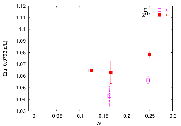
In Fig.2, we compare scaling behaviours between the (naive) lattice SSF $\Sigma(u,a/L)$ and the 1-loop improved one $\Sigma^{(1)}(u,a/L)$ for the RG-improved gauge action with the tree-level value of $c_{t}$ at the weak coupling ($u=0.9793$, left) and the strong coupling ($u=3.3340$, right). Here $\Sigma^{(k)}(u,a/L)$, whose lattice artifacts are perturbatively removed at k-loop, is defined by

where $\delta_{n}$ $(n=1,2\ldots)$ is given by

and $\delta_{1}(a/L)$ for the RG improved action is given in Ref.[6, 3].

Since the scaling violation of $\Sigma^{(1)}$ is milder than that of $\Sigma$, in particular at $u=0.9793$, we hereafter use $\Sigma^{(1)}$ for the continuum extrapolation.

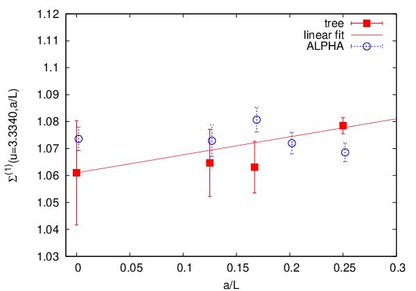
In Fig.3, we compare our $\Sigma^{(1)}$ with $\Sigma^{(2)}$ from the ALPHA Collaboration, where $\Sigma^{(2)}$ is the 2-loop improved lattice SSF, and observe that our errors of $\Sigma^{(1)}$ are larger in general. We think that these larger errors are caused partly by lower statistics and partly by wider widths of distributions mentioned in the previous section. In the figure we also plot linear continuum extrapolations of $\Sigma^{(1)}$, which give $\sigma(u=0.9793)=1.061(19)$ with $\chi^{2}/{\rm dof}=1.74$ and $\sigma(3.3340)=4.91(58)$ with $\chi^{2}/{\rm dof}=0.585$. These values are consistent with results from the ALPHA Collaboration, $\sigma(u=0.9793)=1.072(4)$ and $\sigma(3.3340)=5.60(16)$, though our errors are much lager as expected from errors of $\Sigma^{(1)}$. Note however that results from the ALPHA Collaboration are obtained from the combined fit with $\Sigma^{(2)}$ at all $u$ by the form $\sigma(u)+\rho^{\rm X-loop}u^{4}(a/L)^{2}$ neglecting a tiny $a/L$ term, therefore errors tend to be smaller than those form the individual fit. Here $X$ is the order of the improvement coefficient $c_{t}$: 1-loop for data at $u$ in the weak coupling region and 2-loop in the strong coupling region[1], and the scaling violation starts at $u^{3}$ (3-loop) in $\Sigma^{(2)}(u)/u$.

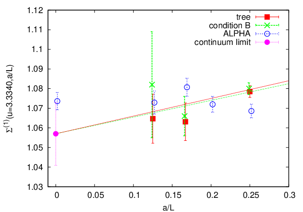
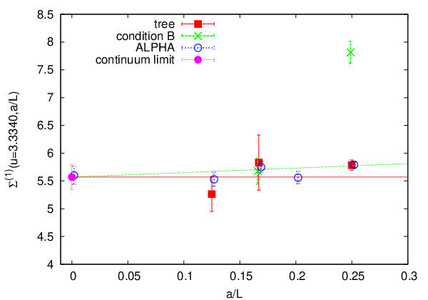
In order to examine scaling behaviours of $\Sigma^{(1)}$ with the RG improved action more precisely, we have repeated the calculation of the SSF using the 1-loop value of boundary improvement coefficients $c_{t}^{P,R}$ with condition B[2]. $\Sigma^{(1)}$ from the 1-loop $c_{t}^{P,R}$ is plotted in Fig.4, together with results from the tree $c_{t}$ and from the ALPHA Collaboration[1]. We observe that three results show mild scaling violations for all $a/L$s’ at the weak coupling(the left figure) , while, in the strong coupling region (the right figure), the scale violation of the result from the 1-loop $c_{t}^{P,R}$ becomes too large at $L/a=4$ to make the reliable continuum extrapolation with this point. A possible reason for this large scaling violation is that the perturbative estimate of $c_{t}^{P,R}$ becomes unreliable in the strong coupling region of the RG-improved action due to the large value of the bare gauge coupling $g_{0}^{2}$. The $\beta$ value which gives the same $u$ is much smaller for the RG-improved action than for the plaquette action. For example, at $u=3.3340$ and $L/a=4$, the RG-improved action needs $\beta=2.1361$ , which corresponds to $g_{0}^{2}=2.8089$ and gives a large(10%) 1-loop correction to $c_{t}^{R}$, $c_{t}^{R(1)}g_{0}^{2}=0.146$. On the other hand, the tree-level value, $c_{t}^{R}$=1.5, remains unchanged for all $\beta$. Since $\bar{g}^{2}_{\rm SF}$ is defined through boundary observables, a small difference in $c_{t}^{P,R}$ may have a large effect on it.

We now perform a combined fit using all our data with tree-level and 1-loop values of $c_{t}^{P,R}$, except one with the 1-loop $c_{t}^{P,R}$ at $L/a=4$ and $u=3.334$. At the weak coupling( $u=0.9793$), we use linear functions in $L/a$ for data with the tree-level value of $c_{t}^{P,R}$( 3 data) and the 1-loop values of $c_{t}^{P,R}$(3 data), while at the strong coupling($u=3.3340$), we use a linear fit for data with the tree-level value of $c_{t}$( 3 data) and a constant fit for data with the 1-loop value of $c_{t}$ excluding one at $L/a=4$( 1 data). From the simultaneous fits shown in Fig. 4, we obtain $\sigma(u=0.9793)=1.057(16)$ with $\chi^{2}/{\rm dof}=1.22$ and $\sigma(u=3.334)=5.57(22)$ with $\chi^{2}/{\rm dof}=2.02$. While both central value and error are almost unchanged at the weak coupling, an agreement with the result from the ALPHA Collaboration becomes better with smaller error at the strong coupling.

We finally make a more complicated combined fit, using our data and fitting functions mentioned above and employing the form $\sigma(u)+\rho^{\rm X-loop}u^{4}(a/L)^{2}$ as fitting functions to data at all $u$ from the ALPHA Collaboration[1]. We obtain $\sigma(u=0.9793)=1.0724(43)$ and $\sigma(u=3.334)=5.559(125)$ with $\chi^{2}/\rm{dof}=2.39$ in the continuum limit. Compared with result from ALPHA Collaboration, 1.0736(44) for weak coupling and 5.60(16) for strong coupling, these errors are reduced by 2% and 22%, respectively.

We have calculated the step scaling function in the SF scheme at weak ($u=0.9793$) and strong ($u=3.3340$) coupling regions with the renormalization group (RG) improved gauge action. Extrapolated values of the SSF from the RG improved gauge action agree with those from the plaquette action within errors at both couplings, though errors of the former are larger.

From a combine fit using all data including ones with the plaquette action from the ALPHA Collaboration[1], we obtain $\sigma(u=0.9793)=1.0724(43)$ and $\sigma(u=3.334)=5.559(125)$ in the continuum limit. These errors are reduced by 2% and 22% from previous results in Ref.[1].

Finally we make two comments on calculations of the SSF with the RG improved gauge action. Firstly, it is better to use the tree-level value of $O(a)$ improvement coefficients $c_{t}^{P,R}$ than the 1-loop value, in particular, in the strong coupling region. Secondly, the HMC algorithm with the RG improved action samples configurations including ones near the secondary minimum better than that with the plaquette action, though statistical fluctuations of $1/\bar{g}^{2}_{\rm SF}$ with the RG improved action become larger.

We are grateful for authors and maintainers of CPS++[10], of which a modified version is used for simulations done in this work. This work was supported in part by the Grant-in-Aid of the Japanese Ministry of Education, Culture, Sports, Science and Technology (Nos. 18740130, 20340047).

References

- [1] M. Della Morte, R. Frezzotti, J. Heitger, J. Rolf, R. Sommer and U. Wolff [ALPHA Collaboration], Nucl. Phys. B 713, 378 (2005) [arXiv:hep-lat/0411025].
- [2] S. Takeda, S. Aoki and K. Ide, Nucl. Phys. Proc. Suppl. 129, 408 (2004) [arXiv:hep-lat/0309160].
- [3] S. Takeda et al., Phys. Rev. D 70, 074510 (2004) [arXiv:hep-lat/0408010].
- [4] S. Aoki et al. [CP-PACS Collaboration and JLQCD Collaboration], Phys. Rev. D 73 (2006) 034501 [arXiv:hep-lat/0508031].
- [5] S. Aoki, R. Frezzotti and P. Weisz, Nucl. Phys. B 540, 501 (1999) [arXiv:hep-lat/9808007].
- [6] S. Sint and R. Sommer, Nucl. Phys. B 465, 71 (1996) [arXiv:hep-lat/9508012].
- [7] K. Murano, S. Aoki, S. Takeda and Y. Taniguchi, in preparation.
- [8] M. Luscher, R. Sommer, P. Weisz and U. Wolff, Nucl. Phys. B 413, 481 (1994) [arXiv:hep-lat/9309005].
- [9] Private communications from S. Sint and R. Sommer for the ALPHA Collaboration.
- [10]
CPS++
http://qcdoc.phys.columbia.edu/chuiwoo_index.html(maintainer: Chulwoo Jung).