Efficient Human Computation: the Distributed Labeling Problem
Abstract
Collecting large labeled data sets is a laborious and expensive task, whose scaling up requires division of the labeling workload between many teachers. When the number of classes is large, miscorrespondences between the labels given by the different teachers are likely to occur, which, in the extreme case, may reach total inconsistency. In this study we describe how globally consistent labels can be obtained, despite the absence of teacher coordination, and discuss the possible efficiency of this process in terms of human labor. We define a notion of label efficiency, measuring the ratio between the number of globally consistent labels obtained and the number of labels provided by distributed teachers. We show that the efficiency depends critically on the ratio between the number of data instances seen by a single teacher, and the number of classes. We suggest several algorithms for the distributed labeling problem, and analyze their efficiency as a function of . In addition, we provide an upper bound on label efficiency for the case of completely uncoordinated teachers, and show that efficiency approaches as the ratio between the number of labels each teacher provides and the number of classes drops (i.e. ).
1 Introduction
As applications of machine learning mature, larger training sets are required both in terms of the number of training instances and the number of classes considered. In recent years we have witnessed this trend for example in vision related tasks such as object class recognition or detection (ghp07; evwwz07; rtmf05). Specifically for object class recognition, current data sets such as the Caltech-256 (ghp07) include tens of thousands of images from hundreds of classes. Collecting consistent data sets of this size is an intensive and expensive task. Scaling up naturally leads to a distributed labeling scenario, in which labels are provided by a large number of weakly coordinated teachers. For example, in the Label-me system (rtmf05) the labels are contributed by dozens of researchers, while in the ESP game (vonAhn06) labels are supplied by thousands of uncoordinated players.
As we turn toward distributed labeling, several practical considerations emerge which may disrupt the data integrity. In general, while it is reasonable to believe that a single teacher is relatively self-consistent (though not completely error-free), this is not the case with multiple uncoordinated teachers. Different teachers may have differences in their labeling systems due to several causes. First, different teachers may use different words to describe the same item class. For example, one teacher may use the word “truck” while the other uses “lorry” to describe the same class. Conversely, the same word may be used by two teachers to describe two totally different classes, hence one teacher may use “greyhound” to describe the breed of dog while the other uses it to describe the C-2 navy aircraft. Similar problems occur when different teachers label the data with different abstraction levels, so one generalizes over all dogs, while the other discriminates between a poodle, a Labrador and etc. Finally, teachers often do not agree on the exact demarcation of concepts, so a chair carved in stone may be labeled as a “chair” by one teacher, while the other describes it as “a rock”. All these phenomena become increasingly pronounced as the number of classes is increased, thus their neglect essentially leads to a severe decrease in label purity and consequently in learning performance.
In this paper we study the cost of obtaining globally consistent labels, while focusing on a specific distributed labeling scenario, in which only some of the difficulties described above are present. To enforce the distributed nature of the problem, we assume that a large data set with examples is to be labeled by a set of uncoordinated teachers, where each teacher agrees to label at most data points. While there is a one-to-one correspondence between the classes used by the different teachers, we assume that their labeling systems are entirely uncoordinated, so a class labeled as “duck” by one teacher may be labeled as a “goat” by another. In later stages of this paper, we relax this assumption, and consider a case in which partial consistency exists between the different teachers. Both scenarios are realistic in various problem domains. Consider for example a security system for which we have to label a large set of face images, including thousands of different people. Since teachers are not familiar with the persons to be labeled, the names they give to classes are entirely un-coordinated. The case of a partial consistency is exemplified in distributed labeling of flower images: the layman can easily distinguish between many different kinds of flowers but can name only a few.
The difficulties of ‘‘one-to-many’’ label correspondence between teachers and concept demarcation disagreements are not met by our current analysis, which focuses on the preliminary difficulties of distributed labeling. Another related scenario, to which our analysis can be extended relatively easily, is the case in which the initial data is labeled by uncoordinated teachers right from the start. Consider for example, the task of unifying images labeled in a site like Flickr11 1 http://www.flickr.com/ into a meaningful large training data set. Our suggested algorithms and analysis apply to this case with minor modifications.
1.1 Relevant literature
In the active learning framework (cal90) and the experimental design framework (see e.g., (ad92)), the goal is to minimize the number of queries for labels (or experiments conducted) while learning a target concept. It has been shown (fsst95) that a careful selection of queries can lead to an exponential reduction in the number of labels needed. This line of research is motivated by the costly and cumbersome process of obtaining labels for instances. We share this motivation but argue that the problem is not merely the quantity of labels but also the quality and the consistency of the labels that should be treated in the data collection process.
The problem of quality of labels, i.e., learning with noise, has been addressed extensively in the machine learning literature (see e.g., (Decatur95)). In this line of work it is assumed that the teacher does not always provide the true instance labels. The severity of noise ranges from adversarial noise, in which the teacher tries to prevent the learning process by providing inaccurate labels, to the more benign random classification noise. While the inconsistency between uncoordinated teachers can be regarded as some form of label noise, it has unique characteristics and its treatment is hence different from the other sources of noise mentioned. Specifically, as long as each teacher is noise-free and self-consistent, we are able to eliminate the noise completely and achieve certain labels.
The scenario of distributed labeling with uncoordinated teachers was considered in the “equivalence constraints” framework (bhsw05). When learning with equivalence constraints, the learner is presented with pairs of instances and the annotation suggests whether they share the same class or not. The authors conjectured that as the number of classes increase, the labeling effort required to coordinate the labels from different teachers becomes prohibitive. We prove this conjecture in Theorem 3. Alternatively, equivalence constraints can be used as a direct supervision for the learning algorithm. Indeed, (bw03) proved that a concept class is learnable with equivalence constraints if it is learnable from labels, so this alternative has some appeal.
1.2 The distributed labeling problem
In the distributed labeling task we have to reveal the labels of instances . We assume that there exist “true” labels (with ) and the distributed labeling algorithm should return such that if and only if . We denote the number of classes by , and assume that each teacher is willing to label only instances where . Throughout this paper we assume that the labels provided by teachers are consistent with the true labels in the sense that for any teacher and any pair of instances
| (1) |
where is the label given by teacher to instance . However, apart from section 4, we assume no inter-teacher consistency with respect to class names, i.e., teachers may disagree on the names of the different classes. To measure the competence of different algorithms for combining the labels of the different teachers we define the following:
Definition 1
Denote by an input sequence of points with the labels . A distributed labeling algorithm is efficient if
where is the average (over the internal randomness of the algorithm) number of human-generated labels the algorithm uses to label the sequence , where each teacher is willing to label examples.
Clearly, if no structural assumptions are made on true labels then is bounded by from above. We denote by the optimal efficiency for a given . I.e., .
1.3 Main results
In section 2 we present several algorithms for solving the distributed labeling problem. The first algorithm presented is the contract the connected components algorithm. We show that this simple algorithms has efficiency of . We then improve this algorithm with the representatives algorithm and prove its efficiency to be better than the efficiency of the previous algorithm. In section 3 we present an upper bound on the achievable efficiency. We show that . In section 4 we study a relaxed version of the distributed labeling problem in which there exists some consistency between the different teachers. Thus, with some probability two teachers will agree on the name of a given class. In this setting, we present a revised version of the algorithm and show its efficiency to be .
2 Label-efficient algorithms
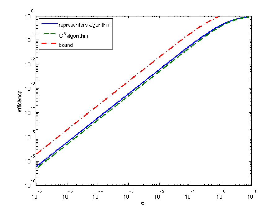
As described in 1.2, we assume in this section that the name each teacher assigns to a class is meaningless. Therefore, the best we can hope for is to break the instances into classes such that any pair of points share the same class label if and only if all teachers give these two points the same label. In this section we suggest two algorithms for this task. The bounds obtained for these algorithms are presented in Figure 1.
2.1 The Contract the Connected Components () algorithm
The first algorithm we consider is the Contract the Connected Components () algorithm presented in Algorithm 1. The idea behind this algorithm is to build a graph whose nodes are sets of equivalent instances. Whenever we find that two nodes share the same label, we contract them into a single node. On the other hand, whenever we find that two nodes do not share the same label, we generate an edge between them. The algorithm ends when the remaining graph is a clique. At this point, each of the nodes is assigned with a unique label. These labels propagate to all the points to be labeled, since each point is associated with a single node in the clique.
input: unlabeled instances
output: a partition of into classes according to the true labels
- 1.
Let be the edge-free graph whose vertexes are .
- 2.
While is not a clique
- (a)
pick random nodes which are not a clique from .
- (b)
send to a teacher and receive .
- (c)
for every do
- i.
if then contract the vertices and in the graph .
- ii.
if then add the edge to the graph .
- i.
- (a)
- 3.
Mark each vertex in with a unique number from .
- 4.
For every vertex in , propagate its label to all the nodes that were contracted into this vertex.
The correctness of the algorithm is straightforward due to the self-consistency of the teachers. In Theorem 1 we show the label efficiency of the algorithm to be where . The main idea behind the analysis is to study the expected number of contractions in each iteration.
Theorem 1
The label efficiency of the algorithm is lower-bounded by
Before proving the theorem, we present a lemma in which the contraction rate associated with a single teacher is bounded.
Lemma 1
Assume a teacher labels random example ( from different classes. The expected number of unique labels that the teacher will give to the instances is at most times where
Note that the number of unique labels is exactly the number of nodes that will be left after contracting the instances.
Proof: Assume that the probability for seeing each of the classes is . The result follows from the following:
| (2) | |||||
| (3) | |||||
The correctness of (3) follows since we are assuming that while is constant.
Proof: (of Theorem 1) At each round of the algorithm, elements are sent to be labeled by a teacher. From Lemma 1 we have that the number of remaining elements is on avarage at most
Therefore, the expected number of rounds the algorithm will make until finished is
Note that the number in the denominator is the expected number of removed elements at each round. Thus, the number of labels used is
Plugging this number into the definition of label efficiency gives the desired result.
2.2 The representatives algorithm
Each teacher provides us with two types of information sources. One is positive equivalence constraints, i.e., the knowledge that two instances share the same label. The other is negative equivalence constraints, i.e., the knowledge that two instances do not share the same label. While the algorithm is very effective in using positive equivalence constraints, it makes very little use of negative equivalence constraints. The representatives algorithm (Algorithm 2) tries to exploit this type of information as well. The main idea behind this algorithm is first to find all the points that belong to certain classes. Once we know that the remaining points do not belong to any of these classes, we are left with a problem with fewer instances and fewer potential classes and thus an “easier one”.
In order to detect all the points belonging to a certain class we use representatives. A representatives set is a set of instances such that for each class there is exactly one member (representative) of the class in the representatives set. Finding a representatives set is a simple task and can be done without affecting the overall efficiency, since its label complexity does not depend on . Therefore, for the sake of simplicity we assume that the representatives set is given in advance. We further assume that we know the probability of each representative class. This information too can be easily estimated from data without jeopardizing efficiency.
Inputs:
- •
unlabeled instances,
- •
a set of representatives such that
- •
a list of probabilities such that is the probability of seeing an instance from the class of .
Outputs: a partition of the points into label classes
- 1.
Reorder the representatives and the ’s such that .
- 2.
Let*
- 3.
Partition the set of representatives into sets classes such that .
- 4.
Let be the edge free graph whose vertices are .
- 5.
While is not empty
- (a)
For
- i.
Partition the remaining points in the graph into sets of size .
- ii.
For each subset of points:
- A.
send these points together with to a teacher.
- B.
contract the graph according to the labels returned by the teacher.
- A.
- iii.
For every
- A.
label with the label , and propogate this label.
- B.
remove from .
- A.
- i.
- (a)
* Choose to optimize the bound in Theorem 2.
is the proportion of representatives in the instances each teacher labels. Note that when , the representative algorithm is essentially the same as the algorithem. However, when , we use the fact that after all the points were compared against a certain representative, we are guaranteed to have found all the points with the same label as this representative, and thus we can eliminate this class.
Theorem 2
The label efficiency of the representative algorithm is lower-bounded by
where is the number of sets in the partition of the representatives into sets and22 2 The function is defined in Lemma 1. .
Proof: In each round of step 5a we break into parts and thus use labels. Therefore, we need only to estimate the size of after each round. Denote the number of vertices in at the beginning of the round by . In order to bound we should consider how it is affected by two ingredients: first the contraction which happen in the same fashion as it happens in the algorithm and the complete elimination of classes .
We use Lemma 1 to analyze the contraction rate. Each teacher sees instances which are not representers of some classes. These instances come from different classes and thus, from Lemma 1 the contraction rate is
Out of the remaining points, all the points which are being represented in are eliminated. Due to the reordering of the s, these points are at least a fraction of of the remaining points. Thus
The number of labels used in all the rounds is therefore
| (4) | |||||
where () is due to the monotonicity of the function. Using the last expression in the efficiency definition completes the proof.
3 The optimal efficiency
In the previous section we studied the efficiency of several algorithms. In the current section we study the efficiency of the optimal algorithm. That is, we study the function
We give an upper bound on showing that algorithms cannot have an efficiency greater than . This bound asserts that the labeling problem is not trivial in the sense that it is not always possible to achieve efficiency 1. Moreover, the problem becomes hard in the limit of , as the efficiency drop linearly with in this region. Comparing the bound shown here and the efficiency of the algorithms presented in previous sections, one can see that there is still a significant gap between the achieved and the (maybe) achievable.
Theorem 3
Let be the best achievable efficiency for a given then
Proof: Fix and and assume . If then the required bound is trivial since efficiency cannot exceed . Therefore, we are only interested in the cases where . Let be a distributed labeling algorithm. For each of the instances we choose a class label uniformly and independently from the possible labels. We analyze the expected number of teacher calls needed before the class assignments are found.
Fix an instance , we first analyze the expected number of teacher calls (in which participates) before it is first contracted with some other point. Assume that has edges in the graph , i.e., there are instances for which it is known that does not share its label. If is a different point than , the probability that they share the same label is at most . To see this, note that for any legal label assignment to , there are at least uplifts of this assignment to .
Let be the probability that is contracted at least once during its first comparisons to other instances. We claim that for all . Clearly, . The proof is by induction. For , clearly the probability for contraction with the first point is compared against is . Note that
In the previous calculation, we assumed that is compared to other points one at a time. However, the teachers label instances at a time, thus whenever is sent to a teacher, it is compared against points. Note that an instance keeps being sent to teachers at least until it is first unified. Therefore, the number of teachers that will have to label until its label is discovered, is at least the total number of teachers that will have to label x until it is unified at least once with another instance. From this we obtain the following lower bound for the expected number of teachers that see x:
The efficiency can be derived from this term
4 Learning with name-consistent teachers
In previous sections we assumed that class names used by different teachers are totally uncoordinated, so naming conventions of one teacher are meaningless to the other. While this scenario may occur (like in the ’face labeling’ task mentioned in the introduction), in most cases this assumption is too pessimistic. It is more reasonable to assume that some level of agreement regarding class names exist, though this agreement is partial and not perfect. In this section we assume that there exist such that with probability over the choice of a random teacher and class , the teacher uses the true global class name as the class label:
| (5) |
We assume some sort of a probability measure over the teachers and the classes. If the pool of teachers is finite, it can be the uniform distribution, and otherwise we assume that whenever we need another teacher to label some instances, the teacher will be such that (5) is true. Notice that we also keep our previous assumption that all the teachers are class consistent in the sense of (1).
When the assumption (5) means that all the teachers use the same global naming system , i.e. for all . In this case the labeling problem is trivial, and it is easy to obtain label efficiency of simply by splitting the instances between different teachers. On the other hand, when is very small, there is no name consistency and the situation boils down to the scenario studied in Section 2. Therefore, we will now focus on studying name consistency in the general case when .
The algorithm we present to address this situation is the Consistently Contract the Connected Components () (Algorithm 3). The difference between the algorithm and the algorithm is that the algorithm sends teachers instances that were previously given the same label by some other teachers.
Input: unlabeled instances
Output: a partition of into classes according to the true labels
- 1.
Let be the edge free graph whose vertices are .
- 2.
Label each vertex with .
- 3.
While is not a clique
- (a)
pick random nodes from such that all these nodes have the same label.
- (b)
send to a teacher and receive .
- (c)
for every , label with the label .
- (d)
for every do
- i.
if then contract the vertices and in the graph .
- ii.
if then add the edge to the graph .
- i.
- (a)
- 4.
Mark each vertex in with a unique number.
- 5.
For every vertex in propagate its label to all the nodes that were contracted into this vertex.
The algorithm differs from the algorithm in using the labels for selecting better candidates for sending to the same teacher. However, note that we still declare the equivalence of two instances only when a single teacher labels both with the same label. Therefore, due to the class consistency (1) the correctness of the algorithm is guaranteed. We now turn to proving its efficiency.
Theorem 4
The label efficiency of the algorithm is lower bounded by
Proof: Following the proof of the efficiency of the algorithm, we compute the rate in which the size of reduces. However, we need to consider two settings. The first applies to teachers that label points for the first time. The second case to consider is teachers who label points that were previously labeled by some other teacher. While these cases may be interleaved in time according to algorithm , w.l.o.g. we may analyze them as if they occur in two consecutive phases.
Following Lemma 1, teachers who label points that were not previously labeled will leave for further process points out of every labeled points. Thus the first phase of labeling will require labels and will leave points in the graph .
In the second phase, each teacher is fed with points that received the same label by different teachers. Due to the name consistency (5) out of points that a teacher labeled we expect of them to have the same label due to the name consistency. The other points are subject to contraction. From Lemma 1 and the above argument we expect that from every points only will remain. The number of labels used by teachers labeling previously labeled points is
Thus, the overall number of labels used is
which leads to the efficiency of
One can easily verify, that if the label efficiency of the algorithm is identical to that of the algorithm. However, the difference between the algorithm and algorithm is profound when and . In this setting, the algorithm has efficiency of while the algorithm is efficient.
Note that despite the remarkable improvment, when there exists complete name consistency and thus it is trivially possible to achieve the perfect efficiency of . However, it is not clear if it is possible to get efficiency close to if is slightly less than . This remains as an open problem.
5 Conclusions and further research
In this work we have studied the problem of generating consistent labels for a large data set given that the labels are provided by restricted teachers. We have focused on the problems arising when the labels used by different teachers are un-coordinated, but nevertheless a one-to-one (unknown) correspondence exists between their labeling systems. In this framework, we provided several algorithms and analyzed their efficiency. We also presented an upper bound which shows that the problem is non-trivial, and becomes hard as the number of classes grows. In the limit we characterize the achievable efficiency to be in the range33 3 The representers algorithm achieves efficiency of with and . To see this, plug these values in (4). , however the exact value remains as an open problem.
We believe that the process of collecting data for large scale learning deserves much attention. One interesting extension of this work is to the case where the symmetry between teachers is broken, either by considering different noise levels to their labels, or more generally, by also allowing the noise level to change between the different classes. In such scenarios, a ’teacher selection’ problem arises as the identity of the teacher can be very informative. One example is the problem of “provost-selection” in which most of the teachers are useless novices in some domain-specific issues and thus it is essential to first find the experts (“provosts”) and use only the labels they provide. A related problem arises when all teachers are useful, but they differ in their discrimination resolutions, so one teacher may say that an image contains a bird while the other may describe the exact bird species. Such problems are left for further research.
References
- Atkinson & Donve, (1992) Atkinson and Donve][1992]ad92 Atkinson, A. C., & Donve, A. N. (1992). optimum experiment designs. Oxford University Press.
- Bar-Hillel et al., (2005) Bar-Hillel et al.][2005]bhsw05 Bar-Hillel, A., Hertz, T., Shental, N., & Weinshall, D. (2005). Learning a mahalanobis metric from equivalence constraints. Journal of Machine Learning Reseach (JMLR), 6(Jun), 937–965.
- Bar-Hillel & Weinshall, (2003) Bar-Hillel and Weinshall][2003]bw03 Bar-Hillel, A., & Weinshall, D. (2003). Learning with equivalence constraints, and the relation to multiclass classification. Conference on Learning Theory (COLT).
- Cohn et al., (1990) Cohn et al.][1990]cal90 Cohn, D., Atlas, L., & Ladner, R. (1990). Training connectionist networks with queries and selective sampling. Advanced in Neural Information Processing Systems 2.
- Decator, (1995) Decator][1995]Decatur95 Decator, S. E. (1995). Efficient learning from faulty data. Doctoral dissertation, Harvard University.
- Everingham et al., (2007) Everingham et al.][2007]evwwz07 Everingham, M., Van Gool, L., Williams, C. K. I., Winn, J., & Zisserman, A. (2007). The PASCAL Visual Object Classes Challenge 2007 (VOC2007) Results. http://www.pascal-network.org/challenges/VOC/voc2007/workshop/index.htm%l.
- Freund et al., (1997) Freund et al.][1997]fsst95 Freund, Y., Seung, H., Shamir, E., & Tishby, N. (1997). Selective sampling using the query by committee algorithm. Machine Learning, 28, 133–168.
- Griffin et al., (2007) Griffin et al.][2007]ghp07 Griffin, G., Holub, A., & Perona, P. (2007). Caltech-256 object category dataset (Technical Report 7694). California Institute of Technology.
- Russell et al., (2005) Russell et al.][2005]rtmf05 Russell, B., Torralba, A., Murphy, K., & Freeman, W. (2005). Labelme: a database and web-based tool for image annotation. mit ai lab memo aim-2005-025.
- von Ahn, (2006) von Ahn][2006]vonAhn06 von Ahn, L. (2006). Games with a purpose. IEEE Computer, 39, 92–94.