Tensor-Entanglement-Filtering Renormalization Approach
and Symmetry Protected Topological Order

Zheng-Cheng Gu Affiliation: Department of Physics, Massachusetts Institute of Technology, Cambridge, Massachusetts 02139, USA Xiao-Gang Wen Affiliation: Department of Physics, Massachusetts Institute of Technology, Cambridge, Massachusetts 02139, USA

Sept., 2008

Abstract

We study the renormalization group flow of the Lagrangian for statistical and quantum systems by representing their path integral in terms of a tensor network. Using a tensor-entanglement-filtering renormalization (TEFR) approach that removes local entanglement and coarse grain the lattice, we show that the resulting renormalization flow of the tensors in the tensor network has a nice fixed-point structure. The isolated fixed-point tensors $T_{\text{inv}}$ plus the symmetry group $G_{\text{sym}}$ of the tensors (ie the symmetry group of the Lagrangian) characterize various phases of the system. Such a characterization can describe both the symmetry breaking phases and topological phases, as illustrated by 2D statistical Ising model, 2D statistical loop gas model, and 1+1D quantum spin-1/2 and spin-1 models. In particular, using such a $(G_{\text{sym}},T_{\text{inv}})$ characterization, we show that the Haldane phase for a spin-1 chain is a phase protected by the time-reversal, parity, and translation symmetries. Thus the Haldane phase is a symmetry protected topological phase. The $(G_{\text{sym}},T_{\text{inv}})$ characterization is more general than the characterizations based on the boundary spins and string order parameters. The tensor renormalization approach also allows us to study continuous phase transitions between symmetry breaking phases and/or topological phases. The scaling dimensions and the central charges for the critical points that describe those continuous phase transitions can be calculated from the fixed-point tensors at those critical points.

I Introduction

For a long time, people believe that all phases and all continuous phase transitions are described by symmetry breaking.[1] Using the associated concepts, such as order parameter, long range correlation and group theory, a comprehensive theory for symmetry breaking phases and their transitions is developed. However, nature’s richness never stops to surprise us. In a study of chiral spin liquid in high temperature superconductor,[2, 3] we realized that there exist a large class of phases beyond symmetry breaking.[4] Since the new phases can be characterized by topology-dependent topologically stable ground state degeneracies, the new type of orders in those phases are named topological orders.[5]. Later, it was realized that fractional quantum Hall states[6] are actually topologically ordered states.[7]

Recently, it was shown that topological order is actually the pattern of long range entanglement in the quantum ground state.[8, 9, 10] The possible patterns of long range entanglement are extremely rich,[11, 12, 13] which indicate the richness of new states of matter beyond the symmetry breaking paradigm. Such rich new states of matter deserve a comprehensive theory.[14, 15]

But how to develop a comprehensive theory of topological order? First we need a quantitative and concrete description of topological order. The topological ground state degeneracy[4, 7] is not enough since it does not completely characterize topological order. However, the non-Abelian Berry’s phases from the degenerate ground states and the resulting representation of modular group provide a more complete characterization of topological order.[5] It may even completely characterize topological order. There are other ways to (partially) characterize topological order, such as through the fractional statistics of the quasiparticles[16, 17] or through the string operators that satisfy the “zero-law”.[18] Those “zero-law” string operators appear to be related to another characterization of topological order through a gauge-like-sysmetry defined on a lower dimensional subspace of the space.[19, 20]

But so far, we have not been able to use those characterizations to develop a theory of topological order. So the key to develop a comprehensive theory of topological order is to find a quantitative and easy-to-use description of topological order. For fractional quantum Hall states, the pattern of zeros appears to provide a quantitative and easy-to-use description of topological order.[21, 22, 23] For more general systems, we may use the renormalization group (RG) approach to find a quantitative and easy-to-use description. We will see that the new description based on the RG approach naturally leads to a theory of topological order and phase transitions between topologically ordered states.

Renormalization group (RG) approach[24, 25] is a powerful method to study phases and phase transitions for both quantum and statistical systems. For example, for a quantum system, one starts with its Lagrangian and path integral that describe the system at a certain cut-off scale. Then one integrates out the short distance fluctuations in the path integral to obtain a renormalized effective Lagrangian at a longer effective cut-off scale. Repeating such a procedure, the renormalized effective Lagrangian will flow to an isolated fixed-point Lagrangian that represents a phase of the system. As we adjust coupling constants in the original Lagrangian, we may cause the renormalization flow to switch from one fixed point to another fixed point, which will represent a phase transition. Since the fixed-point Lagrangian is unique for each phase and the phase transition is associated with a change in fixed-point Lagrangian, it is natural to use the fixed-point Lagrangian to describe various phases.

But can we use the fixed-point Lagrangian to quantitatively describe topological order? At first sight, the answer appears to be no. When a quantum spin system (or a qbit system) has a topologically ordered ground state, its low energy effective Lagrangian (ie the fixed-point Lagrangian) can be a $Z_{2}$ gauge theory,[26, 27, 28, 29, 30] a $U(1)$ gauge theory,[31, 29, 32, 33] a $SU(2)$ gauge theory,[29] a QED theory (with $U(1)$ gauge field and massless fermion field),[29, 34, 35] a QCD theory (with non-Abelian gauge fields and massless fermion fields),[36, 37, 29, 34] a Chern-Simons theory,[3, 38] etc . In the standard implication of RG approach (within the frame work of field theory), a bosonic Lagrangian that describes a quantum spin system cannot flow to all those very different possible fixed-point Lagrangian with very different fields (such as gauge fields and anticommuting fermionic fields).

Since lattice spin systems do have those very different topologically ordered phases, we see that the standard implementation of the RG approach is incomplete and needed to be generalized to cover those existing (and exciting) renormalization flows that end at very different fixed-point Lagrangian. In this paper, we will describe one such generalization – tensor network renormalization approach – that should allow us to study any phases (both symmetry breaking and topological phases) of any systems (with a finite cut-off). The resulting fixed-point Lagrangian from the tensor network renormalization approach give us a quantitative description of topological orders (and the symmetry breaking orders).

The tensor network renormalization approach is based on an observation that the space-time path integral of a quantum spin system or the partition function of a statistical system on lattice can be represented by a tensor trace over a tensor network after we discretize the time and the fields:

\displaystyle\int D\varphi(\textbf{\emph{x}},t)\hskip 1.0pt\mathrm{e}^{-\int{\cal L}}=\sum_{\{\phi_{\textbf{\emph{i}}}\}}\prod T_{\phi_{\textbf{\emph{i}}}\phi_{\textbf{\emph{j}}}\phi_{\textbf{\emph{k}}}\phi_{\textbf{\emph{l}}}}\equiv\text{tTr}\otimes_{\textbf{\emph{i}}}T

(1)

where i label the discretized space-time points and $\phi_{\textbf{\emph{i}}}$ is the discretized field (for detail, see (2)). The different choices of tensor $T_{\phi_{\textbf{\emph{i}}}\phi_{\textbf{\emph{j}}}\phi_{\textbf{\emph{k}}}\phi_{\textbf{\emph{l}}}}$ in the tensor network correspond to different Lagrangians/partition-functions. We like to point out that in addition to use it to describe path integral or partition function, tensor network can also be used to describe many-body wave functions.[39] Based on such a connection, many variational approaches were developed.[39, 40, 41, 42, 43, 44, 45]

Since every physical system is described by path integral, so if we can calculate the tensor trace, we can calculate anything. Unfortunately, calculating the tensor-trace tTr is an NP hard problem in 1+1D and higher dimensions.[46] In , Levin and Nave introduced a tensor renormalization group procedure where a coarse graining of the tensor network is performed to produce a new tensor on the coarse grained network. This leads to an efficient and accurate calculation path integral (or partition function) and other measurable quantities. Such a method opens a new direction in numerical calculation of many-body systems.

The above tensor renormalization group procedure also gives rise to a renormalization flow of the tensor. However, the fixed-point tensor obtained from such a flow is not isolated: even starting with different Lagrangian (ie the tensors) that describe the same phase, the renormalization flow of the those Lagrangian will end up at different fixed-point tensors. This means that the renormalization procedure does not filter out (or integrate out) all the short distance fluctuations so that the fixed-point tensors still contain short distance non-universal information. In this paper, we will introduce an improved tensor renormalization group procedure by adding a filtering operation that remove the local entanglements. We show that this additional entanglement filtering procedure fixes the above problem, at least for the cases studied in this paper.

To test the new tensor network renormalization method, we study the fixed-point tensors that correspond to the two phases of 2D statistical Ising model which has a $Z_{2}$ spin flip symmetry. We find that the fixed-point tensor for the disordered phase is a trivial tensor $T^{\text{TRI}}$ where the dimensions of all the tensor indices are equal to one (we will refer such a trivial tensor as a dimension-one tensor which is represented by a number). While the fixed-point tensor for the symmetry breaking (spin ordered) phase is a dimension-two tensor $T^{Z_{2}}$ which is a direct sum of two dimension-one tensors: $T^{Z_{2}}=T^{\text{TRI}}\oplus T^{\text{TRI}}$ . We believe that this is a general feature for symmetry breaking phase: a symmetry breaking phase with $n$ degenerate states is represented by fixed-point tensors that is a direct sum of $n$ dimension-one trivial tensors.

Since the $Z_{2}$ spin flip symmetry is crucial for the existence and the distinction of the disordered phase and the spin ordered phase, we should use a pair, the symmetry group $G_{\text{sym}}=Z_{2}$ and the fixed-point tensors $T_{\text{inv}}=T^{\text{TRI}},\ T^{Z_{2}}$ , to characterize the two phases. So the disordered phase is characterized by $(Z_{2},T^{\text{TRI}})$ and the spin ordered phase is characterized by $(Z_{2},T^{Z_{2}})$ . It turns out that the characterization based on the symmetry group and the fixed-point tensor, $(G_{\text{sym}},T_{\text{inv}})$ , is very general. It can describe both symmetry breaking phases and topological phases. This is one of the main results of this paper.

Even at the critical point between the symmetry breaking phases and/or topological phases, the tensor renormalization approach produces fixed-point tensors (which now have an infinite dimension). From those fixed-point tensors, or more precisely, from a finite-dimension approximation of those fixed-point tensors, we can calculate the critical properties of the critical points with an accuracy of 0.1%. Using such an method, we confirm that the phase transition between the disordered and ordered phases of the Ising model is a central charge $c=1/2$ critical point.

We also study a 2D statistical loop gas model. We find that for the small-loop phase, the fixed-point tensor is the dimension-one tensor $T^{\text{TRI}}$ , while for the large loop phase, the fixed-point tensor $T^{\text{LL}}$ is a tensor with dimension 2 (see (24)). However, unlike the symmetry breaking phase, the fixed-point tensor for the large loop phase is not a direct sum of two dimension-one tensors: $T^{\text{LL}}\neq T^{\text{TRI}}\oplus T^{\text{TRI}}$ . This is consistent with the fact that, as a statistical system, the small-loop phase and the large loop phase has the same symmetry and the phase transition is not a symmetry breaking transition. The example demonstrates that fixed-point tensors can be used to study phases and phase transitions beyond symmetry breaking. The phase transition between the two phases is again a central charge $c=1/2$ critical point.

Next, we study a spin-1/2 model $H=\sum_{i}(-\sigma^{x}_{i}\sigma^{x}_{i+1}-J\sigma^{z}_{i}\sigma^{z}_{i+1})$ , with $Z^{x}_{2}\times Z^{z}_{2}$ symmetry generated by $\hskip 1.0pt\mathrm{i}\hskip 1.0pt\sigma^{x}$ and $\hskip 1.0pt\mathrm{i}\hskip 1.0pt\sigma^{z}$ . The spin-1/2 model has two different $Z_{2}$ symmetry breaking phases described by, in terms of the new notation, $(Z^{x}_{2}\times Z^{z}_{2},T^{Z_{2}})$ and $(Z^{x}_{2}\times Z^{z}_{2},T^{\text{LL}})$ . The $(Z^{x}_{2}\times Z^{z}_{2},T^{Z_{2}})$ phase breaks the $Z^{x}_{2}$ symmetry while the $(Z^{x}_{2}\times Z^{z}_{2},T^{\text{LL}})$ phase breaks the $Z^{z}_{2}$ symmetry. The phase transition between the two $Z_{2}$ symmetry breaking phases is a continuous phase transition that is beyond the Landau symmetry breaking paradigm. We find that the tensor network renormalization approach can describe such a continuous phase transition. The phase transition between the two phases is a central charge $c=1$ critical point.

Last we study the $T=0$ phases of quantum spin-1 model in 1+1D $H=-\sum_{i}[\textbf{\emph{S}}_{i}\cdot\textbf{\emph{S}}_{i+1}+U(S^{z}_{i})^{2}+BS^{x}_{i}]$ , and found that the model has four different phases for different $(U,B)$ : a trivial phase, two $Z_{2}$ symmetry breaking phases, and the Haldane phase.[48, 49, 50] We find that the Haldane phase is described by a dimension-four fixed-point tensor $T^{\text{Haldane}}$ (see (31)). $T^{\text{Haldane}}$ is not a direct sum of dimension-one tensors. From the fixed-point tensor $T^{\text{Haldane}}$ , we confirm that the Haldane phase has a finite energy gap and the ground state is not degenerate. Thus, despite the fixed-point tensor to be a dimension-four tensor, the Haldane phase, like the trivial phase, does not break any symmetry (as expected).

The TEFR approach allows us to study the stability of the Haldane phase (ie the distinction between the Haldane phase and the trivial phase) under a very general setting. Our calculation shows that the fixed-point tensor $T^{\text{Haldane}}$ , and hence, the Haldane phase is robust against any perturbations that have time-reversal, parity, and translation symmetries.¹¹ 1 When we say the Haldane phase is robust against certain perturbations, we mean that, even in the presence of those perturbations, the Haldane phase is still separated from the trivial $S^{z}=0$ phase by phase transitions. So the Haldane phase is a symmetry protected topological phase characterized by the pair $(G_{TPT},T^{\text{Haldane}})$ where $G_{TPT}$ is the symmetry group generated by time-reversal, parity, and translation symmetries.

People have been using the degenerate spin-1/2 degrees of freedom at the ends of spin-1 chain,[51, 52, 53] and string order parameter[54, 55] to characterize Haldane phase. Both degenerate boundary spin-1/2 degrees of freedom and the string order parameter can be destroyed by perturbations that break spin rotation symmetry but have time-reversal, parity, and translation symmetries. So if we used the degenerate spin-1/2 degrees of freedom and/or string order parameter to characterize the Haldane phase, we would incorrectly conclude that the Haldane phase is unstable against those perturbations. Since the Haldane phase is indeed stable against those perturbations, we conclude that the $(G_{TPT},T^{\text{Haldane}})$ characterization is more general. We also find that an arbitrary small perturbation that break parity symmetry will destabilize the Haldane phase. This confirms a previously known result.[56]

In the first a few sections of this paper, we will review and introduce several tensor network renormalization approaches. Then we will discuss new physical picture about phases and phase transitions emerged from the tensor network renormalization approach through several simple examples.

Refer to caption — Figure 1: A graphic representation of a tensor-network on a square lattice. A vertex represent a tensor $T_{ijfe}$ and the legs of a vertex carries the indices $i$ , $j$ , etc . Each link carries the same index. The indices on the internal links are summed over, which defines the tensor-trace.

II A review of a tensor network renormalization method

In the following review, we will concentrate on 1+1D quantum systems. However, our discussion can be generalized to 2D statistical systems and the systems in higher dimensions.

To describe the tensor renormalization approach introduced in , we first note that, after we discretize the space-time, the partition function represented by a space-time path integral ${\rm Tr}\hskip 1.0pt\mathrm{e}^{-\beta H}=\int\hskip 1.0pt\mathrm{e}^{-\int{\cal L}}$ (in imaginary time) can be written as a tensor-trace over a tensor-network (see Fig. 1 for an example on 2D square lattice):

{\rm Tr}\hskip 1.0pt\mathrm{e}^{-\beta H}=\sum_{ijkl\cdots}T_{jfei}T_{hgjk}T_{qklr}T_{lits}\cdots=\text{tTr}\otimes_{\textbf{\emph{i}}}T.

(2)

where the indices of the tensor run from $1$ to $D$ (in other words the tensor $T$ is a rank-four dimension- $D$ tensor). Choosing different tensors $T$ corresponds to choosing different Lagrangian ${\cal L}$ . We see that calculating the tensor trace allows us to obtain properties of any physical systems.

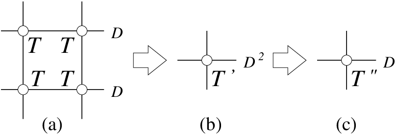
Unfortunately, calculating the tensor-trace tTr is an NP hard problem in 1+1D and higher dimensions.[46] To solve this problem, introduced an approximate real-space renormalization group approach which accelerate the calculation exponentially. The basic idea is quite simple and is illustrated in Fig. 2. After finding the reduced tensor $T^{\prime\prime}$ , we can express $\text{tTr}[T\otimes T\cdots]\approx\text{tTr}[T^{\prime\prime}\otimes T^{\prime\prime}\cdots]$ where the second tensor-trace only contains a quarter of the tensors in the first tensor-trace. We may repeat the procedure until there are only a few tensors in the tensor-trace. This allows us to reduce the exponential long calculation to a polynomial long calculation.

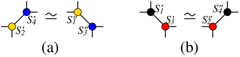
The actual implementation of the renormalization is a little more involved.[47, 45] For an uniform tensor-network on 2D square lattice (see Fig 1), the renormalization group procedure can be realized in two steps. The first step is decomposing the rank-four tensor into two rank-three tensors. We do it in two different ways on the sublattice purple and green (see Fig. 4a). On purple sublattice, we have $T_{ruld}=\sum_{s=1}^{D^{2}}{S_{1}}_{uls}{S_{3}}_{drs}$ and on green sublattice, we have $T_{ruld}=\sum_{s=1}^{D^{2}}{S_{2}}_{lds}{S_{4}}_{rus}$ . Note that $r,l,u,d$ run over $D$ values while $s$ run over $D^{2}$ values. For such a range of $s$ , the decomposition can always be exact.

Next we try to reduce the range of $s$ through an approximation.[47] Say, on purple sublattice, we view $T_{ruld}$ as a matrix $M_{lu;rd}^{\rm{p}}=T_{ruld}$ and do singular value decomposition

\displaystyle M^{\rm{p}}=U\Lambda V^{\dagger},\ \ \ \ \ \Lambda=\begin{pmatrix}\lambda_{1}&&&\\ &\lambda_{2}&&\\ &&&\ddots\\ \end{pmatrix}

(3)

where $\lambda_{1}>\lambda_{2}>\lambda_{3}$ … We then keep only the largest $D_{cut}$ singular values $\lambda_{s}$ and define ${S_{3}}_{drs}=\sqrt{\lambda_{s}}V^{\dagger}_{s,rd}$ , ${S_{1}}_{uls}=\sqrt{\lambda_{s}}U_{lu,s}$ . Thus, we can approximately express $T_{ruld}$ by two rank-three tensors $S_{1}$ , $S_{3}$

\displaystyle T_{ruld}\simeq\sum_{s=1}^{D_{\rm{cut}}}{S_{1}}_{uls}{S_{3}}_{drs}.

(4)

Similarly, on green sublattice we may also define $T_{ruld}$ as a matrix $M_{ld;ru}^{\rm{g}}$ and do singular value decompositions, keep the largest $D_{\text{cut}}$ singular values and approximately express $T_{ruld}$ by two rank-three tensors $S_{2},S_{4}$ .

\displaystyle\mathbb{T}_{\alpha\beta\mu\nu}\simeq\sum_{\gamma=1}^{D_{\rm{cut}}}{S_{2}}_{\nu\alpha\gamma}{S_{4}}_{\beta\mu\gamma}

(5)

After such decompositions, the square lattice is deformed into the form in Fig. 4b. The second step is simply contract the square and get a new tensor $T^{\prime}$ on the coarse grained lattice (see Fig. 3b). The dimension for the reduced tensor $T^{\prime}$ is only $D_{\text{cut}}$ which can be chosen to be $D$ or some other values. This defines the (approximated) renormalization flow of the tensor network based on the SVD. Let us call such an approach SVD based tensor renormalization group (SVDTRG) approach.

III The physical meaning of fixed-point tensors

Why the SVDTRG flow fails to produce a isolated fixed-point tensors? Levin has pointed out that one large class of tensors – corner double-line (CDL) tensors – are fixed points of the SVDTRG flow.[47, 57] A CDL tensor has a form (see Fig. 5a)

	$\displaystyle T_{ruld}(M^{1},M^{2},M^{3},M^{4})$	$\displaystyle=T_{r_{1}r_{2},u_{2}u_{1},l_{2}l_{1},d_{1}d_{2}}$
		$\displaystyle=M^{1}_{r_{2}u_{1}}M^{2}_{u_{2}l_{1}}M^{3}_{l_{2}d_{1}}M^{4}_{d_{2}r_{1}}$		(6)

where the pair $(r_{1},r_{2})$ represents the index $r$ , etc . Such type of tensor (assuming $\sqrt{D}=$ integer and $r_{1}$ etc run from $1$ to $\sqrt{D}$ ) has exact decomposition

\displaystyle T_{ruld}

\displaystyle=\sum_{s=1}^{D_{\text{cut}}}{S_{3}}_{drs}{S_{1}}_{lus}=\sum_{s=1}^{D_{\text{cut}}}{S_{2}}_{lds}{S_{4}}_{rus}

with $D_{\text{cut}}=D$ . This makes the CDL tensor to be the fixed-point tensor under the SVDTRG flow at least when $M^{1}=M^{2}=M^{3}=M^{4}$ . If the initial tensor is changed slightly, the tensor may flow to a slight different CDL tensor, and hence the fixed point is not isolated.

A tensor network of CDL tensor is plotted in Fig. 5b. If the system described by a tensor network does flow to a tensor network of CDL tensor, what does this means? From Fig. 5b, we see that, at the fixed point described by the CDL tensor, the degrees of freedom form clusters that correspond to the disconnected squares. Only the degrees of freedom within the same square interact and there are no interactions between different clusters. Such a fixed-point tensor (ie Lagrangian) describes a system with no interaction between neighbors and has a finite energy gap. So the system is in a trivial phase without symmetry breaking and without topological order (in the sense of long range entanglement). The $h\gg J$ phase of the transverse-field Ising model

H_{\text{tIsing}}=-\sum_{i}(J\sigma^{x}_{i}\sigma^{x}_{i+1}+h\sigma^{z}_{i})

(7)

is such a phase. We can check that the tensor network that describes the above transverse-field Ising model indeed flows to a network of CDL tensor when $h\gg J$ .

On the other hand, the low energy physics of such phases is really trivial. $J=0$ and $h=\infty$ limit, the partition function of the transverse-field Ising model is described by a dimension-one tensor

\displaystyle T^{\text{TRI}}_{ruld}=\delta_{r,1}\delta_{u,1}\delta_{l,1}\delta_{d,1}

(8)

Thus we expect that the fixed-point tensor for the $h\gg J$ phase should be the above trivial dimension-one tensor. Unfortunately, the renormalization flow generated by SVDTRG fails to produce such simple fixed-point tensor.

The $h\ll J$ phase of the transverse-field Ising model is a symmetry breaking phase with two degenerate ground states. Under the SVDTRG flow, the tensor network of the transverse-field Ising model will flow to a tensor network described by a tensor of the form

\displaystyle T=T_{\text{cdl}}\oplus T_{\text{cdl}}

(9)

where $T_{\text{cdl}}$ is a CDL tensor. On the other hand, the symmetry breaking phase should be described by a simpler tensor eqn. (9) where $T_{cdl}$ is the dimension-one tensor $T^{\text{TRI}}$ given by eqn. (8).

However, the SVDTRG flow does a remarkable job of squeezing all the complicated entanglement into a single plaquette! Note that the initial tensor network may contain entanglement between lattice sites separated by a distance less than the correlation length. A CDL tensor contains only entanglement between nearest-neighbor lattice sites, while the ideal fixed-point tensor eqn. (8) has no entanglement at all (not even with next neighbors).

What should be the fixed-point tensor for topological phases under SVDTRG flow? The essence of topological phases is pattern of long-range entanglement.[8, 9, 10] Since the CDL tensor has no long range entanglement, its cannot be used to describe topologically ordered phases. We believe that topological phases are described by fixed-point tensors of the following form (see Fig. 6)

\displaystyle T=T_{cdl}\otimes T_{top}

(10)

where $T_{cdl}$ is CDL tensor and $T_{top}$ is a tensor that cannot be decomposed further as $T_{top}=T^{\prime}_{cdl}\otimes T^{\prime}_{top}$ . Here $T_{top}$ will be the fixed-point tensor that characterizes the topological order.

IV Filtering out the local entanglements

We have seen that the SVDTRG flow can produce a network of CDL tensor which squeezes the non-topological short range entanglement into single plaquette. To obtain ideal fixed-point tensor (such as the one in eqn. (8)) we need to go one step further to remove the corner entanglement represented by the CDL tensor, ie we need to reduce corner matrix $M^{i}$ in the CDL tensor (see eqn. (8)) to a simpler form

\displaystyle M^{i}_{ab}\to\delta_{a,1}\delta_{b,1}.

(11)

In the following, we will describe one way to do so.

In this approach, we modify the SVDTRG transformation described by Fig. 4 to a new transformation described by Fig. 7. We will call the new approach tensor-entanglement-filtering renormalization (TEFR) approach. In the TEFR transformation, we first deform the square lattice Fig. 7(a) into the lattice Fig. 7(b) by expressing the rank-four tensor $T$ in terms of two rank-three tensors $S_{1},S_{3}$ or $S_{2},S_{4}$ [see Fig. 3(a)]. Then we replace the four rank-three tensors $S_{1},S_{2},S_{3},S_{4}$ by a new set of simpler rank-three tensors $S^{\prime}_{1},S^{\prime}_{2},S^{\prime}_{3},S^{\prime}_{4}$ so that the tensor trace of $S^{\prime}_{1},S^{\prime}_{2},S^{\prime}_{3},S^{\prime}_{4}$ (approximately) reproduces that of $S_{1},S_{2},S_{3},S_{4}$ as shown in Fig. 8. In this step, we try to reduce the dimensions of the rank-three tensors, from $D\times D\times D$ of $S_{i}$ to $D\times D\times D^{\prime}$ of $S^{\prime}_{i}$ with $D^{\prime}<D$ . If $T$ is a CDL tensor, $S_{1},S_{2},S_{3},S_{4}$ will also be CDL tensors [see Fig. 10(a)]. In this case, the above procedure will result in a new set of tensors $S^{\prime}_{1},S^{\prime}_{2},S^{\prime}_{3},S^{\prime}_{4}$ with a lower dimension as shown in Fig. 10(b). (For details, see Appendix .1.) We then use the SVD (see Fig. 9) to deform the lattice in Fig. 7(c) to that in Fig. 7(d). Last we trace out the indices on the small squares in Fig. 7(d) to produce new tensor network on a coarse grained square lattice [see 7(e)] with a new tensor $T^{\prime}$ . The tensor $T^{\prime}$ will have a lower local entanglement than $T$ . In fact, when $T$ is a CDL tensor, the combined procedures described in Fig. 4 and Fig. 7 (see also Fig. 10 and 11) can reduce $T$ to a dimension-one tensor. Appendix .1 contains a more detailed description of TEFR method.

V Examples

In the section, we will apply the TEFR method to study several simple well known statistical and quantum systems to test the TEFR approach. We will calculate the free energy (for statistical systems) or the ground-state energy (for quantum systems). The singularities in free-energy/ground-state-energy in the large system limit will indicate the presence of phase transitions. We can also calculate the fixed-point tensors under the TEFR flow for each phase. The fixed-point tensors will allow us to identify those phases as symmetry breaking and/or topological phases. If we find a continuous phase transition in the above calculation, we can also use the fixed-point tensor at the critical point to calculate the spectrum of the scaling dimensions $h_{i}$ and the central charge $c$ for the critical point (see Appendix .2).

V.1 2D statistical Ising model

Our first example is the 2D statistical Ising model on square lattice described by

H=-\sum_{\langle\textbf{\emph{i}},\textbf{\emph{j}}\rangle}\sigma_{\textbf{\emph{i}}}\sigma_{\textbf{\emph{j}}},\ \ \ \ \ \sigma_{\textbf{\emph{i}}}=\pm 1

(12)

where $\sum_{\langle\textbf{\emph{i}},\textbf{\emph{j}}\rangle}$ sums over nearest neighbors. The partition function is given by $Z={\rm Tr}(e^{-\beta H})$ . Such a partition function can be expressed as a tensor-trace over a tensor-network on a (different) square lattice where the tensor $T$ is given by

$\displaystyle T^{\text{Ising}}_{1,2,1,2}$	$\displaystyle=e^{-4\beta},$	$\displaystyle T^{\text{Ising}}_{2,1,2,1}$	$\displaystyle=e^{-4\beta},$
$\displaystyle T^{\text{Ising}}_{1,1,1,1}$	$\displaystyle=e^{4\beta},$	$\displaystyle T^{\text{Ising}}_{2,2,2,2}$	$\displaystyle=e^{4\beta},$
others	$\displaystyle=1.$			(13)

Note that the spins are located on the links of the tensor-network (ie i in (12) labels the links of the tensor-network).

The statistical Ising model has a $Z_{2}$ spin flip symmetry. Such a symmetry implies that the tensor is invariant under the following $Z_{2}$ transformation

\displaystyle T^{\text{Ising}}_{ruld}=W_{rr^{\prime}}W_{uu^{\prime}}W_{ll^{\prime}}W_{dd^{\prime}}T^{\text{Ising}}_{r^{\prime}u^{\prime}l^{\prime}d^{\prime}},

(14)

where

\displaystyle W=\begin{pmatrix}0&1\\ 1&0\\ \end{pmatrix}.

We performed 14 steps of TEFR iteration described in Fig. 7 with $D_{\text{cut}}=32$ . The calculated free energy $F=-\beta^{-1}\log(Z)=-T\log(Z)$ is presented in Fig. 12. For temperature $T>2.38$ , the fixed-point tensor is a dimension-one tensor

\displaystyle T^{\text{TRI}}_{1111}=1,\ \ \ \ \ \ \ \text{others}=0.

(15)

For temperature $T<2.19$ , the fixed-point tensor is a dimension-two tensor

\displaystyle T^{Z_{2}}_{1111}=1,\ \ \ \ \ \ \ T^{Z_{2}}_{2222}=1,\ \ \ \ \ \ \ \text{others}=0.

(16)

For temperature $2.22<T<2.32$ , the fixed-point tensor is complicated with many non-zero elements. (We like to point out that the above fixed-point tensors are actually invariant fixed-point tensors. For details, see Appendix .2.)

To visualize the structure of fixed-point tensors more quantitatively in different regions, we introduce the following two quantities (see Fig. 13)

\displaystyle X_{1}

\displaystyle=\frac{(\sum_{ru}T_{ruru})^{2}}{\sum_{ruld}T_{rulu}T_{ldrd}},

\displaystyle X_{2}

\displaystyle=\frac{(\sum_{ru}T_{ruru})^{2}}{\sum_{ruld}T_{ruld}T_{ldru}}

(17)

for the fixed-point tensors. Note that $X_{1}$ and $X_{2}$ is independent of the scale of the tensor $T\to\Gamma T$ . We plotted $X_{1}$ , $X_{2}$ and the central charge obtained from (53) for the fixed-point tensors $T_{\text{inv}}$ at different temperatures in Fig. 14. (Note that $\tau_{0}=\tau_{1}=\hskip 1.0pt\mathrm{i}\hskip 1.0pt$ here.) We see that the different values of $X_{1}$ and $X_{2}$ mark the different phases, and the steps in $X_{1}$ and $X_{2}$ , as well as the peak in $c$ mark the point of continuous transition.

From the structure of the fixed-point tensor, we see that the low-temperature phase $T<2.19$ is a $Z_{2}$ symmetry breaking phase (where the fixed-point tensor has a form $T^{Z_{2}}=T^{\text{TRI}}\oplus T^{\text{TRI}}$ ) and the high-temperature phase $T>2.38$ is a trivial disordered phase. Since $\partial F/\partial T$ appear to be continuous and $\partial^{2}F/\partial T^{2}$ appears to have an algebraic divergence at the transition point, all those suggest that the phase transition is a continuous transition, which is a totally expected result. From the Onsager’s solution[58] $\text{sinh}(2/T_{c})=1$ , one obtains the exact critical temperature to be $T_{c}=\frac{2}{\log(\sqrt{2}+1)}=2.26919$ , which is consistent with our numerical result.

There is another interpretation of the fixed-point tensors. The fixed-point in the low temperature phase $T^{Z_{2}}=T^{\text{TRI}}\oplus T^{\text{TRI}}$ happen to be the initial tensor (13) in the zero temperature limit $\beta=\infty$ . Thus the flow of the tensor in the low temperature phase can be viewed as a flow of the temperature $\beta\to\infty$ . Using the same reasoning, we expect that the flow of the tensor in the high temperature phase can also be viewed as a flow of temperature $\beta\to 0$ in the opposite direction. This would suggest that the fixed-point tensor should have a form

\widetilde{T}^{\text{TRI}}_{ruld}=\frac{1}{4},\ \ \ \ r,u,l,d=1,2

(18)

which is very different from the trivial dimension-one tensor $T^{\text{TRI}}$ in (15). We will explain below that the two tensors $\widetilde{T}^{\text{TRI}}$ and $T^{\text{TRI}}$ are equivalent.

To see the equivalence, we would like to point out that two tensors $T$ and $T^{\prime}$ related by

\displaystyle T^{\prime}_{r^{\prime}u^{\prime}l^{\prime}d^{\prime}}=(A^{-1})_{l^{\prime}l}(B^{-1})_{u^{\prime}u}T_{ruld}A_{rr^{\prime}}B_{dd^{\prime}}

(19)

give rise to same tensor trace for any square-lattice tensor network. In particular, if the singular values in the SVD decomposition in Fig. 3(a) has degeneracies, the coarse grained tensor will have the ambiguity described by the above transformation with $A$ and $B$ being orthogonal matrices. Physically, the transformation (19) corresponds to a field redefinition. One can check explicitly that

\widetilde{T}^{\text{TRI}}_{ruld}=R^{-1}_{rr^{\prime}}R^{-1}_{uu^{\prime}}T^{\text{TRI}}_{r^{\prime}u^{\prime}l^{\prime}d^{\prime}}R_{l^{\prime}l}R_{d^{\prime}d}

where

R=\frac{1}{\sqrt{2}}\begin{pmatrix}1&1\\ 1&-1\end{pmatrix}

(20)

Thus, $\widetilde{T}^{\text{TRI}}$ and $T^{\text{TRI}}$ are equivalent under a field redefinition.

We have seen that the coarse grained tensors after the TEFR transformations may contain a field redefinition ambiguity (19). As a result, the $Z_{2}$ transformation on the coarse grained lattice may be different from that on the original lattice. The $Z_{2}$ transformation on the coarse grained lattice is related to the original $Z_{2}$ transformation by a field redefinition transformation.

However, one can choose a basis on the coarse grained lattice by doing a proper field-redefinition transformation such that the $Z_{2}$ spin flip transformation has the same form on the coarse grained lattice as that on the original lattice. In such a basis, the disordered and the $Z_{2}$ symmetry breaking phases are described by $(G_{\text{sym}},T_{\text{inv}})=(Z_{2},\widetilde{T}^{\text{TRI}})$ and $(G_{\text{sym}},T_{\text{inv}})=(Z_{2},T^{Z_{2}})$ , respectively, where the $Z_{2}$ transformation is given by (14). This example shows how to use the pair $(G_{\text{sym}},T_{\text{inv}})$ to describe the two phases of the statistical Ising model.

Next we like to use the fixed-point tensor $T_{\text{inv}}$ at the critical point to calculate the critical properties of the above continuous transition. We can use (49) to obtain the invariant fixed-point tensor $T^{(i)}_{\text{inv}}$ even off the critical point. From $T^{(i)}_{\text{inv}}$ we calculate the matrices $M^{ud}$ , $M^{lr}$ , $M^{ldru}$ , and $M^{lurd}$ from (50), and obtain the eigenvalues $\lambda_{n}$ of those matrices. Using those eigenvalues, we can calculate the central charge and the scaling dimensions from (53), where $\tau=\tau_{1}=\hskip 1.0pt\mathrm{i}\hskip 1.0pt$ for the Ising model discussed here. By choosing $D_{\text{cut}}=64$ and doing 9 iterations of Fig. 7 (that correspond to a system with 1024 spins) at the critical temperature $T_{c}=\frac{2}{\log(\sqrt{2}+1)}$ , we find that

$\displaystyle c$	$\displaystyle h_{1}$	$\displaystyle h_{2}$	$\displaystyle h_{3}$	$\displaystyle h_{4}$
$\displaystyle 0.49942$	$\displaystyle 0.12504$	$\displaystyle 0.99996$	$\displaystyle 1.12256$	$\displaystyle 1.12403$
$\displaystyle 1/2$	$\displaystyle 1/8$	$\displaystyle 1$	$\displaystyle 9/8$	$\displaystyle 9/8$

where we also listed the exact values of the central charge and the scaling dimensions. We would like to mention that the TEFR approach does not suppose to work well at the critical point where the truncation error of keeping only a finite $D_{\text{cut}}$ singular values is large. It turns out that for $D_{\text{cut}}=64$ , the estimated relative truncation error is less than $10^{-5}$ through $9$ iterations. This allows us to obtain quite accurate central charge and scaling dimensions. The truncation error will grow for more iterations. As a result, the agreement with the exact result will worsen.

From this example, we see that the TEFR approach is an effective and efficient way to study phases and phase transitions. The TEFR approach allow us to identify spontaneous symmetry breaking from the structure of fixed-point tensors. The critical properties for the continuous phase transition can also be obtained from the fixed-point tensor at the critical point.

V.2 2D statistical loop-gas model

Next we consider a 2D statistical loop-gas model on square lattice. The loop-gas model can be viewed as a Ising model with spins on the links of the square lattice. However, the allowed spin configurations must satisfies the following hard constraint: the number of up-spins next each vertex must be even. The energy of spin configuration is given by

H=-\sum_{\langle\textbf{\emph{i}}\rangle}\sigma_{\textbf{\emph{i}}}

(21)

The partition function $Z={\rm Tr}(e^{-\beta H})$ can be expressed as a tensor-trace over a tensor-network on the square lattice where the tensor $T$ is given by

	$\displaystyle T^{\text{LG}}_{ruld}$	$\displaystyle=\hskip 1.0pt\mathrm{e}^{\beta(2d-3)/2}\hskip 1.0pt\mathrm{e}^{\beta(2u-3)/2}\hskip 1.0pt\mathrm{e}^{\beta(2r-3)/2}\hskip 1.0pt\mathrm{e}^{\beta(2l-3)/2}\times$
		$\displaystyle\ \ \ \ \ \ \delta_{d+u+r+l=\text{even}}$		(22)

where the indices take the values $r,u,l,d=1,2$ and

\delta_{d+u+r+l=\text{even}}=1\ \ \text{ if }d+u+r+l=\text{even},\ \ \ \ \text{others}=0.

To use the TEFR approach to calculate the partition function, it is very important to implement the TEFR in such a way that the closed-loop condition

	$\displaystyle T_{ruld}$	$\displaystyle=0,\text{ when }r+u+l+d=\text{odd}$
	$\displaystyle S_{rul}$	$\displaystyle=0,\text{ when }r+u+l=\text{odd}$		(23)

are satisfied at every step of iteration.

We performed 14 steps of TEFR iteration described in Fig. 7 with $D_{\text{cut}}=32$ . Fig. 15 shows the resulting $X_{1}$ , $X_{2}$ , and the central charge $c=\frac{6}{\pi}\log(\lambda_{0})$ obtained from (53) for the invariant fixed-point tensors $(T_{\text{inv}})_{ruld}$ at different temperatures. We find that the low temperature phase is described by the trivial dimension-one fixed-point tensor $T^{\text{TRI}}$ (8) as indicated by $X_{1}=X_{2}=1$ . The high temperature phase has a non-trivial fixed-point tensor since $X_{1}=X_{2}=2$ . We find that the invariant fixed-point tensor to have a form

	$\displaystyle T^{\text{LL}}_{ruld}$	$\displaystyle=\frac{1}{2},\text{ if }l+r+u+d=\text{even},\ \ r,u,l,d=1,2$
	others	$\displaystyle=0.$		(24)

The two fixed-point tensors $T^{\text{TRI}}$ and $T^{\text{LL}}$ correspond to the zero-temperature and infinite-temperature limit of the initial tensor $T^{\text{LG}}$ in (22). Both fixed-point tensors satisfy the closed-loop condition (23).

It is well known that the high temperature phase of the statistical loop gas model is dual to the low temperature phase of the statistical Ising model, and the low temperature phase of the statistical loop gas model is dual to the high temperature phase of the statistical Ising model. The fixed-point tensors of the two models are related directly

	$\displaystyle T^{\text{LL}}_{ruld}$	$\displaystyle=R^{-1}_{rr^{\prime}}R^{-1}_{uu^{\prime}}T^{Z_{2}}_{r^{\prime}u^{\prime}l^{\prime}d^{\prime}}R_{l^{\prime}l}R_{d^{\prime}d}$
	$\displaystyle T^{\text{TRI}}_{ruld}$	$\displaystyle=R^{-1}_{rr^{\prime}}R^{-1}_{uu^{\prime}}\widetilde{T}^{\text{TRI}}_{r^{\prime}u^{\prime}l^{\prime}d^{\prime}}R_{l^{\prime}l}R_{d^{\prime}d}$

where $R$ is given in (20). The critical properties at the continuous transition are also identical.

One may wonder, if $T^{\text{LL}}$ and $T^{Z_{2}}$ are related by a field redefinition, then why the TEFR flow produces $T^{\text{LL}}$ as the fixed-point tensor of the high temperature phase of the loop gas, rather than $T^{Z_{2}}$ ? Indeed, if we implement the TEFR flow in the space of generic tensors, then both $T^{\text{LL}}$ and $T^{Z_{2}}$ , together with many other tensors related by some field redefinitions will appear as the fixed-point tensors of the high temperature phase of the loop gas. However, if we implement the TEFR flow in the space of tensors that the describe closed loops (ie satisfying (23)), then only $T^{\text{LL}}$ will appear as the fixed-point tensor.

V.3 Generalized 2D statistical loop-gas model

Third, let us discuss a more general 2D statistical loop-gas model described by a tensor network with tensor

\displaystyle T^{\text{GLG}}_{ruld}

\displaystyle=\hskip 1.0pt\mathrm{e}^{-(r+l+u+d-6)\beta+V\delta_{rlud}}\delta_{d+u+r+l=\text{even}},

(25)

where $r,u,l,d=1,2$ and $\delta_{rlud}$ is given by

\delta_{1111}=\delta_{2222}=1,\ \ \ \ \text{others}=0.

We note that when $V=0$ , the generalized loop-gas model become the one discussed above: $T^{\text{LG}}=T^{\text{GLG}}|_{V=0}$ .

Let us consider the phases of the generalized loop-gas model along the $\beta=0$ line. In this case, the loop-gas model also has a $Z_{2}$ symmetry: the tensor $T^{\text{GLG}}$ is invariant under switching the 1 and 2 index:

	$\displaystyle T^{\text{GLG}}_{ruld}$	$\displaystyle=W_{rr^{\prime}}W_{uu^{\prime}}W_{ll^{\prime}}W_{dd^{\prime}}T^{\text{GLG}}_{r^{\prime}u^{\prime}l^{\prime}d^{\prime}},$
	$\displaystyle W_{x}$	$\displaystyle=\begin{pmatrix}0&1\\ 1&0\\ \end{pmatrix}.$		(26)

We will call such a symmetry $Z^{x}_{2}$ symmetry. The closed-loop condition (23) can also be represented as a $Z_{2}$ symmetry of the tensor:

	$\displaystyle T^{\text{GLG}}_{ruld}$	$\displaystyle=W_{rr^{\prime}}W_{uu^{\prime}}W_{ll^{\prime}}W_{dd^{\prime}}T^{\text{GLG}}_{r^{\prime}u^{\prime}l^{\prime}d^{\prime}},$
	$\displaystyle W_{z}$	$\displaystyle=\begin{pmatrix}1&0\\ 0&-1\\ \end{pmatrix}.$		(27)

The second $Z_{2}$ symmetry will be called $Z^{z}_{2}$ symmetry. So along the $\beta=0$ line, the model has a $Z^{x}_{2}\times Z^{z}_{2}$ symmetry.

We performed the TEFR calculation for the generalized loop-gas model along the $\beta=0$ line with $D_{\text{cut}}=32$ . Fig. 16 shows the $V$ dependence of the resulting log partition function per tensor, $logz=log(Z)/N$ , and $d^{2}logz/dV^{2}$ . Fig. 17 and Fig. 18 show the $V$ dependence of $X_{1}$ , $X_{2}$ , and central charge $c$ for the resulting fixed-point tensor. We see that there is a phase transition at $V_{c}=1.0985$ . The fixed-point tensor for the $V<V_{c}$ phase is found to be $T^{\text{LL}}$ and the fixed-point tensor for the $V>V_{c}$ phase is found to be $T^{Z_{2}}$ . The central charge is zero for the two phases on the two sides of the transition. Thus the both phases have short range correlations. Using the $(G_{\text{sym}},T_{\text{inv}})$ notation, the two phases are characterized by $(Z^{x}_{2}\times Z^{z}_{2},T^{\text{LL}})$ and $(Z^{x}_{2}\times Z^{z}_{2},T^{Z_{2}})$ .

Since $\partial\log(Z)/\partial V$ has no discontinuous jump at $V_{c}$ , the transition is a continuous phase transition. Also the central charge is non zero at the transition point which suggests that the correlation length diverges at $V_{c}$ . This also implies that the transition is a continuous phase transition. From Fig. 18, we see that the transition is a central charge $c=1$ critical point.

We note that the two fixed-point tensors $T^{\text{LL}}$ and $T^{Z_{2}}$ give rise to the same $X_{1}$ and $X_{2}$ . In fact, $T^{\text{LL}}$ and $T^{Z_{2}}$ are related by a field-redefinition transformation (19):

T^{\text{LL}}_{ruld}=R^{-1}_{rr^{\prime}}R^{-1}_{uu^{\prime}}T^{Z_{2}}_{r^{\prime}u^{\prime}l^{\prime}d^{\prime}}R_{l^{\prime}l}R_{d^{\prime}d}

where $R$ is given in (20). Since $X_{1}$ and $X_{2}$ are invariant under the above transformation, so they are the same in the two phases.

The generalized loop-gas model provides us an interesting example that the fixed-point tensors $T^{\text{LL}}$ and $T^{Z_{2}}$ that describe the two phases are related by a field redefinition transformation. In this case, one may wonder should we view the $V<V_{c}$ and $V>V_{c}$ phases as the same phase? A simple direct answer to the above question is no. It is incorrect to just use a fixed-point tensors to characterize a phase. We should use the pair $(G_{\text{sym}},T_{\text{inv}})$ to characterize a phase. If we use the $(G_{\text{sym}},T_{\text{inv}})$ notation, the two phases are more correctly described by $(Z^{x}_{2}\times Z^{z}_{2},T^{\text{LL}})$ and $(Z^{x}_{2}\times Z^{z}_{2},T^{Z_{2}})$ . The above field-redefinition transformation transforms $T^{\text{LL}}$ to $T^{Z_{2}}$ . It also transform the symmetry transformations $Z^{x}_{2}\times Z^{z}_{2}$ to a different form $\widetilde{Z}^{x}_{2}\times\widetilde{Z}^{z}_{2}$ . Thus the pair $(Z^{x}_{2}\times Z^{z}_{2},T^{\text{LL}})$ is transformed to $(\widetilde{Z}^{x}_{2}\times\widetilde{Z}^{z}_{2},T^{Z_{2}})$ under the above field-redefinition transformation. Therefore, we cannot transform the pair $(Z^{x}_{2}\times Z^{z}_{2},T^{\text{LL}})$ to $(Z^{x}_{2}\times Z^{z}_{2},T^{Z^{2}})$ using any field redefinition transformation. This implies that the two phases $(Z^{x}_{2}\times Z^{z}_{2},T^{\text{LL}})$ and $(Z^{x}_{2}\times Z^{z}_{2},T^{Z_{2}})$ are different if we do not break the $Z^{x}_{2}\times Z^{z}_{2}$ symmetry. If we do break the $Z^{x}_{2}\times Z^{z}_{2}$ symmetry, then the two phases are characterized by $(1,T^{\text{LL}})$ and $(1,T^{Z_{2}})$ , where $1$ represents the trivial group with only identity implying that the system has no symmetry. Without any symmetry, the two labels $(1,T^{\text{LL}})$ and $(1,T^{Z_{2}})$ are related under a field redefinition transformation. This implies that the two phases $(1,T^{\text{LL}})$ and $(1,T^{Z_{2}})$ are the same phase if the system has no symmetry. In Appendix .3, we will give a more detailed and general discuss about the definition of phases and its relation to the symmetry of the system.

V.4 Quantum spin-1/2 chain and phase transition beyond symmetry breaking paradigm

The generalized loop-gas model is closely related to the following 1D quantum spin-1/2 model:

H=\sum_{i}[-\sigma^{x}_{i}\sigma^{x}_{i+1}-J\sigma^{z}_{i}\sigma^{z}_{i+1}-h\sigma^{z}_{i}]

(28)

Note that $\sum(1-\sigma^{z}_{i})/2=\sum_{i}n_{i}$ mod 2 is a conserved quantity and the above model can be viewed as a 1D hard-core boson model with next neighbor interaction. Such a 1D quantum model can be simulated by a 2D statistical loop-gas model described by a tensor network with tensor $T^{\text{GLG}}$ (25). The loops in the loop gas correspond to the space-time trajectories of the hard-core bosons. The $\beta=0$ limit of the loop-gas model correspond to $h=0$ limit of the 1D quantum model, and $V$ corresponds to $J$ .

In the following, we will concentrate on the $h=0$ case. When $h=0$ , the Hamiltonian (28) has a $Z^{x}_{2}\times Z^{z}_{2}$ symmetry, where $Z^{x}_{2}$ is the $Z_{2}$ group generated by $\sigma^{x}$ and $Z^{z}_{2}$ is the $Z_{2}$ group generated by $\sigma^{z}$ . Such a $Z^{x}_{2}\times Z^{z}_{2}$ symmetry corresponds to the $Z^{x}_{2}\times Z^{z}_{2}$ symmetry discussed in last section.

When $J<J_{c}=1$ , the system is in a symmetry breaking phase. We will use a pair of groups $(G_{\text{sym}},G_{\text{grnd}})$ to label such a symmetry breaking phase, where $G_{\text{sym}}$ is the symmetry group of the Hamiltonian and $G_{\text{grnd}}$ is the symmetry group of a ground state. So the $J<J_{c}$ phase of our system is labeled by $(G_{\text{sym}},G_{\text{grnd}})=(Z^{x}_{2}\times Z^{z}_{2},Z^{x}_{2})$ , where the ground state breaks the $Z^{z}_{2}$ symmetry but has the $Z^{x}_{2}$ symmetry. When $J>J_{c}$ , our system is in a different symmetry breaking phase, which is labeled by $(G_{\text{sym}},G_{\text{grnd}})=(Z^{x}_{2}\times Z^{z}_{2},Z^{z}_{2})$ .

Under the correspondence between the loop gas and our quantum spin-1/2 model, the $V<V_{c}$ and $V>V_{c}$ phases of the loop-gas model discussed above will correspond to the above two $Z_{2}$ symmetry breaking phases for $J<J_{c}=1$ and $J>J_{c}$ respectively. The results from the loop gas imply that the two $Z_{2}$ symmetry breaking phases are connected by a continuous phase transition. Such a continuous phase transition can be viewed as two $Z_{2}$ symmetry breaking transition happening at the same point.

Strictly speaking, the above continuous transition does not fit within the standard symmetry breaking paradigm for continuous phase transitions. According to Landau symmetry breaking theory, a continuous phase transition can only happen between two phases labeled by $(G_{\text{sym}},G_{\text{grnd}})$ and $(G_{\text{sym}},G^{\prime}_{\text{grmd}})$ where $G_{\text{grnd}}$ is a subgroup of $G_{\text{grnd}}^{\prime}$ or $G_{\text{grnd}}^{\prime}$ is a subgroup of $G_{\text{grnd}}$ . We see that the continuous transition between the $(Z^{x}_{2}\times Z^{z}_{2},Z^{x}_{2})$ phase and $(Z^{x}_{2}\times Z^{z}_{2},Z^{z}_{2})$ phase does not fit within the standard Landau symmetry breaking theory. Such a continuous transition is another example of continuous transitions that is beyond the Landau symmetry breaking paradigm.[59, 60, 61, 62, 63, 29, 64] Even though the above continuous phase transition does not fit within the standard symmetry breaking theory, such a transition can still be studied through the tensor network renormalization approach. In particular, the tensor network renormalization approach reveals that the transition is a central charge $c=1$ critical point.

V.5 Quantum spin-1 chain

Last, we consider a quantum spin-1 chain at zero temperature. The Hamiltonian is given by

H=\sum_{i}\left(\textbf{\emph{S}}_{i}\cdot\textbf{\emph{S}}_{i+1}+U(S^{z}_{i})^{2}+BS^{x}_{i}\right)

(29)

The model has a translation symmetry, a $Z_{2}$ time reversal symmetry $S^{y}\to-S^{y}$ and $Z_{2}$ parity symmetry. The imaginary-time path-integral of the model can be written as

\displaystyle{\rm Tr}\hskip 1.0pt\mathrm{e}^{-\tau H}=\lim_{M\to\infty}{\rm Tr}(\ e^{-\delta\tau H_{e}}e^{-\delta\tau H_{o}})^{M}

where $\delta\tau=\tau/M$ and

	$\displaystyle H_{e}$	$\displaystyle=\sum_{i=\text{even}}\Big(\textbf{\emph{S}}_{i}\cdot\textbf{\emph{S}}_{i+1}+U(S^{z}_{i})^{2}+\frac{B}{2}(S^{x}_{i}+S^{x}_{i+1})\Big)$
	$\displaystyle H_{o}$	$\displaystyle=\sum_{i=\text{odd}}\Big(\textbf{\emph{S}}_{i}\cdot\textbf{\emph{S}}_{i+1}+U(S^{z}_{i})^{2}+\frac{B}{2}(S^{x}_{i}+S^{x}_{i+1})\Big)$

Note that $H_{e}$ and $H_{o}$ are sum of non overlapping terms and thus

	$\displaystyle\hskip 1.0pt\mathrm{e}^{-\delta\tau H_{e}}$	$\displaystyle=\prod_{i=\text{even}}\hskip 1.0pt\mathrm{e}^{-\delta\tau H_{i}}$
	$\displaystyle\hskip 1.0pt\mathrm{e}^{-\delta\tau H_{o}}$	$\displaystyle=\prod_{i=\text{odd}}\hskip 1.0pt\mathrm{e}^{-\delta\tau H_{i}}.$

$H_{i}$ in the above expression has a form

\displaystyle H_{i}=\textbf{\emph{S}}_{i}\cdot\textbf{\emph{S}}_{i+1}+U(S^{z}_{i})^{2}+\frac{B}{2}(S^{x}_{i}+S^{x}_{i+1})

The matrix elements of $\hskip 1.0pt\mathrm{e}^{-\delta\tau H_{i}}$ can be represented by a rank-four tensor (see Fig. 19)

\displaystyle T_{m_{i+1},m_{i},m^{\prime}_{i},m^{\prime}_{i+1}}=(\hskip 1.0pt\mathrm{e}^{-\delta\tau H_{i}})_{m_{i}m_{i+1},m^{\prime}_{i}m^{\prime}_{i+1}},

(30)

where $m_{i},m^{\prime}_{i}$ label of the quantum states of $\textbf{\emph{S}}_{i}$ . Therefore the imaginary-time path-integral ${\rm Tr}\hskip 1.0pt\mathrm{e}^{-\tau H}$ can be expressed as a tensor trace over a tensor network of $T$ (see Fig. 20(a))

\displaystyle{\rm Tr}\hskip 1.0pt\mathrm{e}^{-\tau H}=\text{tTr}\otimes_{i}T.

Now we can use the TEFR approach to evaluate the tensor trace and to obtain the fixed-point tensors. This allows us to find the zero-temperature phase diagram and the quantum phase transitions of the spin-1 model (29).

However, for small $\delta\tau$ , the tensor network is very anisotropic with very different correlation lengths (measured by the distance of the tensor network) in the time and the space directions. This causes large truncation errors in the TEFR steps Fig. 7(a) $\to$ (b) and Fig. 7(c) $\to$ (d) [or Fig. 3(a)]. We need to perform anisotropic coarse graining to make the system more or less isotropic before performing the TEFR coarse graining. One such anisotropic coarse graining in time direction is described in Fig. 20. Each coarse graining step of Fig. 20 triple the effective $\delta\tau$ . After making the effective $\delta\tau$ to be of order 1, we switch to the isotropic coarse graining in Fig. 7.

We performed 11 steps of TEFR iteration in Fig. 2 (which is implemented as 22 steps of TEFR iteration in Fig. 7) with $D_{\text{cut}}=37$ for various value of $U$ and $B$ . After the TEFR iteration, a initial tensor $T(U,B)$ flows to a fixed-point tensor. As we vary $U$ and $B$ , the different initial tensors may flow to different fixed-point tensors which represent different phases. A more detailed description of the renormalization flow of the tensors can be found in Appendix .4.

To quantitatively plot the fixed-point tensors, we can use $X_{1}$ , $X_{2}$ (see (17)) , and $\lambda_{\text{sum}}$ . Here $\lambda_{\text{sum}}$ is given by $\lambda_{\text{sum}}=\sum_{s}|\lambda_{s}/\lambda_{1}|$ and $\lambda_{i}$ are the singular values of the matrix $M^{lurd}$ obtained from the fixed-point tensor (see (50) and (3)). In Fig. 21, we plot the $X_{1}$ , $X_{2}$ , and $\lambda_{\text{sum}}$ of the resulting fixed-point tensors for different value of $U$ and $B$ .

We see that our spin-1 system has four different phases: TRI, $Z^{z}_{2}$ , $Z^{y}_{2}$ , and Haldane. The transition between the Haldane phase and the $Z_{2}$ phase happens at $B_{c}=0.405$ along the $U=0$ line, which agrees with the Haldane gap $\Delta=0.4097=B_{c}$ obtained in . The transition between the Haldane phase and the TRI phase happens at $U_{c}=1.0$ along the $B=0$ line, which agrees with the result $U_{c}=0.99$ obtained in .

The fixed-point tensor in the TRI phase is the trivial dimension-one tensor $T^{\text{TRI}}$ with $(X_{1},X_{2},\lambda_{\text{sum}})=(1,1,1)$ . So the TRI phase has no symmetry breaking. The fixed-point tensor in the $Z^{y}_{2}$ and $Z^{z}_{2}$ phase, up to a field redefinition transformation, are the dimension-two tensor $T^{Z_{2}}$ which is a direct sum of two dimension-one tensor $T^{\text{TRI}}$ with $(X_{1},X_{2},\lambda_{\text{sum}})=(2,2,2)$ . So the $Z^{y}_{2}$ and the $Z^{z}_{2}$ phases are $Z_{2}$ symmetry breaking phases. The fixed-point tensor in the Haldane phase is a dimension-four tensor. However, many different dimension-four tensors can appear as the fixed-point tensors. All those dimension-four fixed-point tensors have $(X_{1},X_{2},\lambda_{\text{sum}})=(1,1,4)$ . In fact they are all equivalent to the following CDL tensor

T^{\text{Haldane}}=T(\sigma^{y},\sigma^{y},\sigma^{y},\sigma^{y})

(31)

through the field-redefinition transformation (19), where $T(\sigma^{y},\sigma^{y},\sigma^{y},\sigma^{y})$ is given in (6). In fact, one can show that the following four CDL tensors, $T(\sigma^{x},\sigma^{x},\sigma^{x},\sigma^{x})$ , $T(\sigma^{y},\sigma^{y},\sigma^{y},\sigma^{y})$ , $T(\sigma^{z},\sigma^{z},\sigma^{z},\sigma^{z})$ , and $T(\sigma^{0},\sigma^{0},\sigma^{0},\sigma^{0})$ , are all equivalent through the field-redefinition transformation. (Here $\sigma^{0}$ is the two by two identity matrix.) So they can all be viewed as the fixed-point tensors in the Haldane phase. Since the fixed-point tensor in the Haldane phase is a CDL tensor, the Haldane phase, like the TRI phase, also does not break any symmetry.

From the fixed-point tensors, we can also obtain the low energy spectrum of our spin-1 system (see Appendix .2). Using the fixed-point tensors of the four phases, we find that all four phases have a finite energy gap. We also find that the ground states of the TRI and Haldane phases are non degenerate while the ground states of the $Z^{y}_{2}$ and $Z^{z}_{2}$ phases have a two-fold degeneracy. This is consistent with our result that the TRI phase and the Haldane phase do not break any symmetry while the $Z^{y}_{2}$ and $Z^{z}_{2}$ phases break a $Z_{2}$ symmetry.

The central charge calculated from the resulting fixed-point tensors is plotted in Fig. 22 (see (53)). The lines of non-zero central charge in Fig. 22 mark the region of diverging correlation length, which correspond to line of continuous phase transition. The energy gap closes along those lines. Compare Fig. 22 with Fig. 21, we see that all the phase transitions in the phase diagram Fig. 21 correspond to those critical lines. Those phase transitions are all continuous phase transitions. The transitions between Haldane and $Z_{2}^{z}$ , Haldane and $Z_{2}^{y}$ , TRI and $Z_{2}^{y}$ , are described by central charge $c=1/2$ critical point. The transitions between $Z_{2}^{y}$ and $Z_{2}^{z}$ , Haldane and TRI, are described by central charge $c=1$ critical point.

The continuous phase transition between the TRI and $Z_{2}$ phases, and between the Haldane and $Z_{2}$ phases are $Z_{2}$ symmetry breaking transitions. The phase transition between the $Z^{y}_{2}$ and the $Z^{z}_{2}$ phases is of the same type as that discussed in section V.4 along the $h=0$ line. Along the $U=0$ line, our spin-1 model has a $U(1)$ spin rotation symmetry around the $S^{x}$ axis. The gapless phase at $B>B_{c}$ and $U=0$ is close to a $U(1)$ symmetry breaking phase where spins are mainly in the $y$ - $z$ plane with a finite and uniform $S_{x}$ component. When $U\neq 0$ , the $U(1)$ spin rotation symmetry is broken. When $U>0$ , the spin-1 model is in the $Z^{y}_{2}$ phase with $S^{y}_{i}\propto(-)^{i}$ . When $U<0$ , the spin-1 model is in the $Z^{z}_{2}$ phase with $S^{z}_{i}\propto(-)^{i}$ .

Both the TRI phase and the Haldane phase have the same symmetry, but yet they are separated by phase transitions. This suggests that the TRI phase and the Haldane phase are distinct phases. But we cannot use symmetry breaking to distinguish the two phases. So let us discuss Haldane phase in more detail.

V.6 Haldane phase – a symmetry protected topological phase

The first question is that weather the TRI phase and the Haldane phase are really different? (For a detail discuss on the definitions of phases and phases transitions, see Appendix .3.) Can we find a way to deform the two phases into each without any phase transition? At first sight, we note that the fixed-point tensor for the Haldane phase are CDL tensors. According to the discussion in section III, this seems to suggest that the Haldane phase is the trivial TRI phase described by $T^{TRI}$ .

In fact, the answer to the above question depend on the symmetry of the Hamiltonian. If we allow to deform the spin-1 Hamiltonian arbitrarily, then the TRI phase and the Haldane phase will belong to the same phase, since the two phases can be deformed into each other without phase transition. If we require the Hamiltonian to have certain symmetries, then the TRI phase and the Haldane phase are different phases (in the sense defined in Appendix .3).

To demonstrate the above result more concretely, let us consider a spin-1 system with time-reversal, parity (spatial reflection), and translation symmetries. The time-reversal symmetry requires the Hamiltonian $H$ and the corresponding tensor $T$ (see 30) to be real. Since the real Hamiltonian must be symmetric, time-reversal symmetric tensor must also satisfy

T_{ruld}=T_{dlur}

(32)

(Note that the time-reversal transformation exchanges $(m_{i},m_{i+1})\leftrightarrow(m^{\prime}_{i},m^{\prime}_{i+1})$ in (30)) The parity symmetry requires the tensor $T$ to satisfy

T_{ruld}=T_{urdl}.

(33)

(Note that the parity exchanges $(m_{i},m^{\prime}_{i})\leftrightarrow(m_{i+1},m^{\prime}_{i+1})$ in (30)) The tensor network considered here is always uniform which ensure the translation symmetry. Our spin-1 Hamiltonian (29) has time-reversal, parity, and translation symmetries.

Using our numerical TEFR calculation, we have checked that the Haldane phase is stable against any perturbations that respect the time-reversal, parity, and translation symmetries. In other words, we start with a tensor $T$ that respects the those symmetries and flows to the fixed-point tensor $T^{\text{Haldane}}$ . We then add an arbitrary perturbation $T\to T+\delta T$ that also respect the time-reversal, parity, and translation symmetries. We find that $T+\delta T$ also flows to the fixed-point tensor $T^{\text{Haldane}}$ as long as $\delta T$ is not too large. This result suggests that the time-reversal, parity, and translation symmetries protect the stability of the Haldane phase. This implies that in the presence of those symmetries, the TRI phase and the Haldane phase are always different. We cannot smoothly deform the Haldane phase into the TRI phase through the Hamiltonian that have the time-reversal, parity, and translation symmetries.

If we add a perturbation $\delta T$ that has time-reversal symmetry but not parity symmetry, our numerical result shows that the perturbed tensor $T+\delta T$ will fail to flow to $T^{\text{Haldane}}$ . Instead, it will flow to the trivial fixed-point tensor $T^{\text{TRI}}$ . This implies that, without the parity symmetry, the Haldane phase is unstable and is the same as the trivial phase TRI, which agrees the result obtained previously in .

To summarize, for Hamiltonian with time-reversal and parity symmetries, the Haldane phase and the TRI phase are different phases, despite both phases do not break any symmetries. So the difference between the Haldane phase and the TRI phase cannot be describe by Landau symmetry breaking theory. In this sense the Haldane phase behaves like the topologically ordered phases.

On the other hand, for Hamiltonian without parity symmetry, the Haldane phase and the TRI phase are the same phase. We see that the Haldane phase exists as a distinct phase only when the Hamiltonian have time-reversal, parity, and translation symmetries. This behavior is very different from the topological phases which are stable against any perturbations, including those that break the parity symmetry. Therefore, we should refer Haldane phase as a symmetry protected topological phase. We like to stress that the Haldane phase is only one of many possible symmetry protected topological phases. Many other symmetry protected topological phases are studied using projected symmetry group in . For example, without symmetry, there is only one kind of $Z_{2}$ spin liquid. In the presence of spin rotation symmetry and the symmetries of square lattice, there are hundreds different $Z_{2}$ spin liquids.[29] All those $Z_{2}$ spin liquids can be viewed as symmetry protected topological phases.

Since the time-reversal, parity, and translation symmetries play such an important role in the very existence of the Haldane phase, it is not proper to characterize the Haldane phase just using the fixed-point tensor $T^{\text{Haldane}}$ . We should use a pair $(G_{TPT},T^{\text{Haldane}})$ to characterize the Haldane phase. Here $G_{TPT}$ is the symmetry group generated the time reversal, parity, and translation transformations. Using the more complete notation, we can say that $(G_{TPT},T^{\text{Haldane}})$ and $(G_{TPT},T^{\text{TRI}})$ correspond to different phases, while $(G_{TT},T^{\text{Haldane}})$ and $(G_{TT},T^{\text{TRI}})$ correspond to the same phase. Here $G_{TT}$ is the symmetry group generated only by the time-reversal and translation transformations. In terms of the new notation, the four phases, TRI, Haldane, and the two $Z_{2}$ , are labeled by $(G_{TPT},T^{\text{TRI}})$ , $(G_{TPT},T^{\text{Haldane}})$ , $(G_{TPT},T^{Z_{2}^{y}})$ . and $(G_{TPT},T^{Z_{2}^{z}})$ . For a more detailed discussion on how the symmetry transformations act on the fixed-point tensor, see Appendix .5

In this paper, we propose to use the pair $(G_{TPT},T^{\text{Haldane}})$ to characterize the Haldane phase – a symmetry protected topological phase. Such a notation allows us to show that the Haldane phase is stable against any perturbations that respect time-reversal, parity, and translation symmetry. We feel that the new characterization capture the essence of Haldane phase. People have proposed several other ways to characterize the Haldane phase. One of them is to use the emergent spin-1/2 boundary spins at the two ends of a segment of the isotropic spin-1 chain in the Haldane phase. However, such a characterization fails to capture the essence of Haldane phase. The Haldane phase still exists in the presence of an uniform magnetic field: $B\sum_{i}S^{z}_{i}$ , while the four-fold degeneracy from the emergent spin-1/2 boundary spins is lifted by such an uniform magnetic field. In the presence of an uniform magnetic field, we can no longer use the degeneracy of the boundary spin-1/2 spins to detect the Haldane phase.

People also proposed to use the string order parameter

\displaystyle\lim_{|i-j|\to\infty}\left\langle S^{z}_{i}e^{\hskip 1.0pt\mathrm{i}\hskip 1.0pt\pi\sum_{k=i+1}^{j-1}S^{z}_{k}}S^{z}_{j}\right\rangle\neq 0

to characterize the Haldane phase. But the string order parameter vanishes in the presence of perturbations that contain odd number of spin operators, such as

	$\displaystyle\delta H$	$\displaystyle=\sum_{i}A_{1}[(S^{z}_{i})^{2}S^{z}_{i+1}+(S^{z}_{i+1})^{2}S^{z}_{i}]$
		$\displaystyle\ \ \ \ +\sum_{i}A_{2}[(S^{x}_{i})^{2}S^{x}_{i+1}+(S^{x}_{i+1})^{2}S^{x}_{i}]$

This is because the total number of $S^{z}=+1$ and $S^{z}=-1$ sites mod 2 is not conserved in the presence of the above perturbation. However, the vanishing string order parameter does not imply the instability of Haldane phase. The above perturbation respects the time-reversal and parity symmetries. The Haldane phase is stable against such a perturbation. Therefore, the string order parameter also fails to capture the essence of Haldane phase.

To illustrate the stability of Haldane phase, we also calculated the phase diagrams of following two spin-1 models. The first model is given by

H=\sum_{i}\left(\textbf{\emph{S}}_{i}\cdot\textbf{\emph{S}}_{i+1}+U(S^{z}_{i})^{2}+B(S^{x}_{i}+S^{z}_{i})\right)

(34)

The phase diagram (the color map plot of $X_{1}$ , $X_{2}$ , and $\lambda_{\text{sum}}$ ) and the central charge are plotted in Figs. 23 and 24. The second model is given by

	$\displaystyle H$	$\displaystyle=\sum_{i}\left(\textbf{\emph{S}}_{i}\cdot\textbf{\emph{S}}_{i+1}+U(S^{z}_{i})^{2}\right)$
		$\displaystyle\ \ \ +\frac{B}{2}\sum_{i}(S^{x}_{i}(S^{z}_{i+1})^{2}+S^{x}_{i+1}(S^{z}_{i})^{2}+2S^{z}_{i})$		(35)

The phase diagram and the central charge are plotted in Figs. 25 and 26.

We see that in both models, the Haldane phase and the TRI phases are separated by phase transitions, indicating the stability of the Haldane phase. (Note that the stability of the Haldane phase is defined by the impossibility to deform the Haldane phase to the TRI phase without a phase transition within a symmetry class of Hamiltonian.) Both the models have time-reversal and parity symmetries. In particular, the second model has only time-reversal and parity symmetries. This suggests that the Haldane phase is stable if the Hamiltonian has time-reversal and parity symmetries.

Before ending this section, we like to point out that the form of the fixe-point tensor of the Haldane phase $T^{\text{Haldane}}=T(\sigma^{y},\sigma^{y},\sigma^{y},\sigma^{y})$ implies the following fixed-point wave function for the Haldane phase. Since the fixed-point tensor $T^{\text{Haldane}}=T(\sigma^{y},\sigma^{y},\sigma^{y},\sigma^{y})$ has a dimension four, the effective degrees of freedom in the fixed-point wave function is four states per site (ie per coarse grained site). The four states can be viewed as two spin-1/2 pseudo spins. The fixed-point wave function is then formed by the pseudo spin singlet dimers between nearest neighbor bonds (see Fig. 27).

VI Summary

In this paper, we introduce a TEFR approach for statistical and quantum systems. We can use the TEFR approach to calculate phase diagram with both symmetry breaking and topological phases. We can also use the TEFR approach to calculate critical properties of continuous transitions between symmetry breaking and/or topological phases. The TEFR approach suggests a very general characterization of phases based on the symmetry group $G_{\text{sym}}$ and the fixed-point tensor $T_{\text{inv}}$ . The $(G_{\text{sym}},T_{\text{inv}})$ characterization can describe both symmetry breaking and topological phases. Using such a characterization and through the stability of the fixed-point tensor, we show that the Haldane phase for spin-1 chain is stable against any perturbations that respect time-reversal, parity, and translation symmetry. This suggests that the Haldane phase is a symmetry protected topological phase.

The TEFR approach introduced here can be applied to any strongly correlated systems in any dimensions. It has a potential to be used as a foundation to study topological phases and symmetry protected topological phases in any dimensions. In this paper, we only demonstrate some basic applications of the TEFR approach through some simple examples. We hope those results will lay the foundation for using the TEFR approach to study more complicated strongly correlated systems in 1+2 and in 1+3 dimensions.

To gain a better understanding of the tensor network renormalization approach, let us compare the tensor network renormalization approach with the block-spin renormalization approach.[24] Let us consider a spin system whose partition function can be represented by a tensor network of a tensor $T(g)$ , where $g$ is a coupling constant of the spin system. After performing a coarse graining of the lattice, the system is described by a coarse grained tensor network of tensor $T^{\prime}$ . The transformation $T(g)\to T^{\prime}$ represent tensor network renormalization flow. In the block-spin renormalization approach, we insist on the coarse grained system have the same form as described by a new coupling constant $g^{\prime}$ . So we try to find a $g^{\prime}$ such that $T(g^{\prime})$ best approximates $T^{\prime}$ . This way, we obtain a block-spin renormalization flow $g\to g^{\prime}$ . We see that tensor network renormalization flow is a transformation in the generic tensor space, while the block-spin renormalization flow is a transformation is the subspace $T(g)$ parameterized by the coupling constant $g$ . We believe that it is this generic flow in the whole tensor space allows the tensor network renormalization approach to describe topological phases.

In this paper, we stress that the fixed-point tensor of the tensor network renormalization flow can be used as a quantitative description of topological order. This is just one aspect of topological order. In fact, theory of topological order has a very rich structure and covers a wide area (see Fig. 28). Turaev-Viro invariant[67] on 3D manifold can be viewed as a tensor trace of the fixed-point tensors for string-net models.[12] Therefore, the tensor network renormalization approach should apply to all time reversal and parity symmetric topological orders in 1+2 dimensions which are described by the string-net condensations.[11, 12] This type of topological order include emergent gauge theory, Chern-Simons theory, and quantum gravity in 1+2 dimensions.[68, 69, 12] The mathematical foundation that classifies this type of fixed-point tensors is the tensor category theory. It is natural to expect that the topological order in 1+3 dimensions and the associated emergent gauge bosons, emergent fermions, and emergent gravitons[34, 70] can also be studied through the tensor network renormalization approach. The tensor network renormalization approach also provides a new way to calculate lattice gauge theories. We see that physics is well inter connected. It appears that the tensor network renormalization is a glue that connects all different parts of physics.

VII Acknowledgements

We would like to thank Michael Levin, Frank Verstraete, and Michael Freedman for many very helpful discussions. This research was supported by the Foundational Questions Institute (FQXi) and NSF Grant DMR-0706078.

Appendix

.1 A detailed discussion of the TEFR algorithm

The key step in the TEFR calculation is the entanglement filtering operation from Fig. 7(b) to Fig. 7(c). In this section we will discuss several ways to implement such an entanglement filtering calculation.

.1.1 The linear algorithm

To find those new $S^{\prime}_{i}$ described in Fig. 8, we may minimize the following cost function:

		$\displaystyle\ \ \ C_{L}=$		(36)
		$\displaystyle\parallel\sum_{ijkl}{S_{1}}_{li\alpha}{S_{2}}_{ij\beta}{S_{3}}_{jk\gamma}{S_{4}}_{kl\delta}-\sum_{ijkl}{S_{1}}^{\prime}_{li\alpha}{S_{2}}^{\prime}_{ij\beta}{S_{3}}^{\prime}_{jk\gamma}{S_{4}}^{\prime}_{kl\delta}\parallel$

where $\alpha,\beta,\delta,\gamma=1,\ldots D$ and $i,j,k,l=1,\ldots D^{\prime}$

This cost function can be minimized by solving a sets of least square problems iteratively. For example, we may first fixed $S^{\prime}_{2},S^{\prime}_{3},S^{\prime}_{4}$ and solve a least square problem for $S_{1}^{\prime}$ , then we fixed $S^{\prime}_{1},S^{\prime}_{3},S^{\prime}_{4}$ to solve a least square problem for $S_{2}^{\prime}$ , etc. In practise, to reduce the trapping by local minima, we may start with $D^{\prime}=D-1$ and gradually decrease $D^{\prime}$ .

.1.2 The nonlinear algorithm

Although the linear algorithm is an efficient way to do the entanglement-filtering calculation in Fig. 8, however, this algorithm could not avoid trapping by local minima in generic case. To solve this problem, here we introduce a non-linear algorithm which can avoid the trapping by local minima.

In the first implementation of TEFR discussed above, we choose $S^{\prime}_{i}$ to minimize the dimension of the one of the index of the rank-three tensors $S^{\prime}_{i}$ . The second implementation of TEFR is still described by Fig. 7. But now we choose $S^{\prime}_{i}$ to minimize the entanglement entropy on the diagonal links in Fig. 7(d).

Let us define the entanglement entropy on a link. We may view the tensor network in Fig. 29, as matrix $M_{i,j}$ where $i=(a,b)$ and $j=(c,d)$ . We then perform an SVD of $M$ which produces the singular values $\lambda_{i}$ that are ordered as $\lambda_{1}\geq\lambda_{2}\geq...\geq 0$ . We call $\lambda_{i}$ the singular values on the horizontal link in Fig. 29. The entanglement entropy on the horizontal link in Fig. 29 is defined as $S=-\sum_{i}\widetilde{\lambda}_{i}\log(\widetilde{\lambda}_{i})$ , where $\widetilde{\lambda}_{i}=\lambda_{i}/\sum\lambda_{i}$ . In the non-linear algorithm, we choose $S^{\prime}_{1}$ , $S^{\prime}_{2}$ , $S^{\prime}_{3}$ , and $S^{\prime}_{4}$ to minimize the following cost function

		$\displaystyle\ \ \ C_{NL}=\lambda S_{\text{sum}}+$		(37)
		$\displaystyle\parallel\sum_{ijkl}{S_{1}}_{li\alpha}{S_{2}}_{ij\beta}{S_{3}}_{jk\gamma}{S_{4}}_{kl\delta}-\sum_{ijkl}{S_{1}}^{\prime}_{li\alpha}{S_{2}}^{\prime}_{ij\beta}{S_{3}}^{\prime}_{jk\gamma}{S_{4}}^{\prime}_{kl\delta}\parallel$

where $S_{\text{sum}}$ is the sum of entanglement entropy on the four diagonal links in Fig. 7(d). Here $\lambda$ should be as small as possible.

We note that when we reduce the entanglement entropy on the diagonal links in Fig. 7(d), the singular values on those diagonal links decay faster. This allows us to drop indices associated with the very small singular values and hence reduce the dimension on those diagonal links. When we use Fig. 3(b) to transform Fig. 7(d) to Fig. 7(e), the resulting tensor $T^{\prime}$ will have a small dimension. This approach can again reduce a CDL tensor $T$ to a trivial dimension-one tensor.

The non-linear algorithm is a very general approach, but the calculation is very expensive. In the paper, we will not use this algorithm.

.1.3 The scaling-SVD algorithm for CDL tensors

In this section, we introduce the third algorithm, which is very simple and efficient. We will call such algorithm scaling-SVD algorithm, which can be used to find $S^{\prime}_{1}$ , $S^{\prime}_{2}$ , $S^{\prime}_{3}$ , and $S^{\prime}_{4}$ in Fig. 8 with smaller dimensions.

In the scaling-SVD algorithm, we introduce four diagonal weighting matrices:

	$\displaystyle w^{12}_{ii^{\prime}}$	$\displaystyle=w_{i}^{12}\delta_{ii^{\prime}};\qquad w^{23}_{jj^{\prime}}=w_{j}^{23}\delta_{jj^{\prime}};$
	$\displaystyle w^{34}_{kk^{\prime}}$	$\displaystyle=w_{k}^{34}\delta_{kk^{\prime}};\qquad w^{41}_{ll^{\prime}}=w_{l}^{41}\delta_{ll^{\prime}};$

on those links $i,j,k,l$ in Fig. 30 and initialize them as $1$ . We first perform the scaling-SVD calculation on the pair $S_{1}$ and $S_{2}$ by introducing a matrix:

M^{12}_{\alpha l;j\beta}=\sum_{i}\sqrt{w_{l}^{41}}{S_{1}}_{li\alpha}{S_{2}}_{ij\beta}\sqrt{w_{j}^{23}}

and do the SVD decomposition $M^{12}=U\Lambda V^{\dagger}$ :

M^{12}_{\alpha l;j\beta}=\sum_{i}U_{\alpha l;i}\Lambda_{i}^{12}V_{j\beta;i}.

We then update $S_{1},S_{2}$ as:

{S_{1}}^{\prime}_{li\alpha}=\sqrt{\Lambda^{12}_{i}}U_{\alpha l;i}/\sqrt{w_{l}^{41}};\qquad{S_{2}}^{\prime}_{ij\beta}=\sqrt{\Lambda^{12}_{i}}V_{j\beta;i}/\sqrt{w_{j}^{23}}

We can update $S_{2},S_{3}$ in the same way, then we can further update $S_{3},S_{4}$ and $S_{4},S_{1}$ . After one loop update for those $S_{i}$ ’s, we update all the weighting factors $w^{12}$ etc as $w^{12}=\Lambda^{12}$ etc on corresponding links.

After several loop iterations, we truncate the smallest singular values of $\Lambda^{12}_{i},\Lambda^{23}_{j},\Lambda^{34}_{k},\Lambda^{41}_{l}$ and obtain new rank-three tensors $S_{1}^{\prime},S_{2}^{\prime},S_{3}^{\prime},S_{4}^{\prime}$ with a smaller dimension $D^{\prime}<D$ on the inner links. If $S_{1}$ , $S_{2}$ , $S_{3}$ , and $S_{4}$ are CDL tensor, we find:

{S_{1}}^{\prime}_{li\alpha}{S_{2}}^{\prime}_{ij\beta}{S_{3}}^{\prime}_{jk\gamma}{S_{4}}^{\prime}_{kl\delta}\propto{S_{1}}_{li\alpha}{S_{2}}_{ij\beta}{S_{3}}_{jk\gamma}{S_{4}}_{kl\delta}

after truncation. By proper normalizing those $S^{\prime}_{i}$ , we can find the solution of

\sum_{ijkl}{S_{1}}_{li\alpha}{S_{2}}_{ij\beta}{S_{3}}_{jk\gamma}{S_{4}}_{kl\delta}-\sum_{ijkl}{S_{1}}^{\prime}_{li\alpha}{S_{2}}^{\prime}_{ij\beta}{S_{3}}^{\prime}_{jk\gamma}{S_{4}}^{\prime}_{kl\delta}\approx 0.

(38)

If $S_{1}$ , $S_{2}$ , $S_{3}$ , and $S_{4}$ are not CDL tensor, the truncated $S^{\prime}_{1}$ , $S^{\prime}_{2}$ , $S^{\prime}_{3}$ , and $S^{\prime}_{4}$ cannot satisfy (38) even after the rescaling of $S^{\prime}_{1}$ , $S^{\prime}_{2}$ , $S^{\prime}_{3}$ , and $S^{\prime}_{4}$ . In this case, we reject the truncated $S^{\prime}_{1}$ , $S^{\prime}_{2}$ , $S^{\prime}_{3}$ , and $S^{\prime}_{4}$ and the scaling-SVD fails to produce simplified tensors. To summarize, the scaling-SVD algorithm can simplify CDL tensors, but not other tensors.

To understand why the above scaling-SVD algorithm can work for CDL tensors, we can consider the simplest CDL tensor $T_{ruld}(M^{1},M^{2},M^{3},M^{4})$ with corner matrices

M^{1}=M^{2}=M^{3}=M^{4}=\begin{pmatrix}1&0\\ 0&x\\ \end{pmatrix}.

where $0<x<1$ .

See in Fig. 31, after one loop iteration, the $4\times 4$ diagonal weighting matrix $w=w_{In}\otimes w_{Out}$ on each link is updated as:

w_{In}=\begin{pmatrix}1&0\\ 0&x\\ \end{pmatrix};\qquad w_{Out}=\begin{pmatrix}1&0\\ 0&x\\ \end{pmatrix}

Where $In$ represents the inner line and $Out$ represent the outer line of the square as show in Fig. 31. However, after $n$ loop iteration, we find:

w_{In}=\begin{pmatrix}1&0\\ 0&x^{n}\\ \end{pmatrix};\qquad w_{Out}=\begin{pmatrix}1&0\\ 0&x\\ \end{pmatrix}

The striking thing is that the weighting matrices on the outer lines are never scaled but the weighting matrices (as well as the singular values on the corresponding link) on the inner lines are scaled to its $n$ power! After enough times of loop iterations, $x^{n}$ can be smaller than the machine error. The inner line can be removed and we successfully filter out those local entanglements in the square. In this paper, we do all our TEFR calculations using this scaling-SVD algorithm.

It also clear that if the corner matrices in a CDL tensor have degenerate eigenvalues, the scaling-SVD cannot simplify such a CDL tensor. This is a desired result, since the degeneracy in the singular values may indecate the presence of topological order (see the discussion at the end of Appendix .4).

.2 Partition function and critical properties from the tensor network renormalization flow of the tensors

In this section, we will give a more detailed discussion about the renormalization flow of the tensor. The more detailed discussion allows us to see the relation between the fixed-point tensor and the energy spectrum for a quantum system. It also allows us to see the relation between the fixed-point tensor at the critical point and the scaling dimensions and central charge of the critical point. To be concrete, we will consider the renormalization transformation described by Fig. 2, which represents a single iteration step. Such an iteration step roughly correspond to two iteration steps described by Fig. 3.

We start with a tensor network formed by $N_{0}=N$ tensors $T^{(0)}=T$ . After $i$ iterations, the tensor network is deformed into a tensor network of $N_{i}$ $T^{(i)}$ -tensors. We formally denote the tensor network renormalization flow as

T^{(i)}\to T^{(i+1)}.

Those tensors satisfy the following defining property

\text{tTr}(\otimes T^{(i)})^{N_{i}}=\text{tTr}(\otimes T^{(i+1)})^{N_{i+1}}.

The scales of the tensors $T^{(i)}$ changes under each iteration. It is more convenient to describe the tensor network renormalization flow in terms of the normalized tensor. The normalized tensor is defined as

{\cal T}^{(i)}=T^{(i)}/\Gamma_{i}

(39)

that satisfies

\sum_{l,u}{\cal T}^{(i)}_{l,l,u,u}=1

In terms of the normalized tensor, after a tensor network renormalization transformation, a tensor network of $N_{i}$ normalized ${\cal T}^{(i)}$ -tensors is transformed into a tensor network of $N_{i+1}$ normalized ${\cal T}^{(i+1)}$ -tensors:

{\cal T}^{(i)}\to f_{i+1}{\cal T}^{(i+1)}.

The $N_{i}$ normalized ${\cal T}^{(i)}$ -tensors and the $N_{i+1}$ $f_{i}{\cal T}^{(i+1)}$ -tensors have the same tensor trace

\text{tTr}(\otimes{\cal T}^{(i)})^{N_{i}}=f_{i+1}^{N_{i+1}}\text{tTr}(\otimes{\cal T}^{(i+1)})^{N_{i+1}}.

(40)

$f_{i}$ is a quantity that can be directly obtained from the numerical tensor network renormalization calculation.

From (39) we see that the partition function at $i^{\text{th}}$ iteration can be expressed as a tensor trace of the normalized tensor ${\cal T}^{(i)}$ up to an over all factor

\displaystyle Z_{i}=\Gamma_{i}^{N_{i}}\text{tTr}(\otimes{\cal T}^{(i)})^{N_{i}}.

(41)

Note that by definition, the partition function is invariant under the tensor network renormalization transformation $Z_{i}=Z_{i+1}$ . From (40), we find that $\Gamma_{i}$ satisfies

\displaystyle\Gamma_{i}^{N_{i}}f_{i+1}^{N_{i+1}}=\Gamma_{i+1}^{N_{i+1}}

(42)

which allows us to calculate $\Gamma_{i}$ from $f_{i}$ . We can keep performing the tensor network renormalization until $N_{i}$ is of order 1. This way, we can calculate the partition function $Z=Z_{i}$ from (41) and (42).

To calculate the density of the log partition function $\log(Z)$ , we need to describe how tensor positions in the tensor network are mapped into the physical coordinates $\textbf{\emph{r}}=(x_{1},x_{2})$ . Let $\textbf{\emph{X}}_{1}$ be the vector in physical space connecting the two neighboring tensors in the horizontal direction and $\textbf{\emph{X}}_{2}$ the vector connecting the two neighboring tensors in the vertical direction (see Fig. 32). Let denote the coordinates of $\textbf{\emph{X}}_{i}$ as

\textbf{\emph{X}}_{\alpha}=\begin{pmatrix}W_{1\alpha}\\ W_{2\alpha}\end{pmatrix},\ \ \ \ \alpha=1,2.

(43)

The two by two matrix $W$ describes the shape of the tensor network.

We note that the tensor network is changed under each iteration. So $W_{\alpha\beta}$ is also changed under each iteration. After the $i^{th}$ iteration, the shape of the resulting tensor network is described by $W^{(i)}_{\alpha\beta}$ , where $W^{(0)}_{\alpha\beta}=W_{\alpha\beta}$ is for the initial tensor network. Under the renormalization transformation described in Fig. 2, $W^{(i)}$ transforms in a simple way

W^{(i+1)}=2W^{(i)}.

which implies $A_{i+1}=4A_{i}$ . Under the renormalization transformation described in Fig. 4, $W^{(i)}$ transforms as

W^{(i+1)}=W^{(i)}\begin{pmatrix}1&1\\ -1&1\\ \end{pmatrix}.

The above recursion relations allow us to calculate $W^{(i)}$ for each step of iteration. Such information will be useful later.

We see that the area occupied by each tensor $T^{(i)}$ after the $i^{th}$ iteration is

A_{i}=\text{det}(W^{(i)})

where $W^{(i)}$ is the two by two matrix formed by $W^{(i)}_{\alpha\beta}$ . It is also clear that

A_{i}N_{i}=A_{i+1}N_{i+1}=A_{\text{tot}}

is the total area of the system.

Let us introduce

z_{i}=\Gamma_{i}^{1/A_{i}}.

(44)

From (42), we see that $z_{i}$ satisfies the following recursion relation

\displaystyle z_{i+1}=z_{i}f_{i+1}^{1/A_{i+1}}.

(45)

\log(z_{i})=\log(z_{0})+\sum_{j=1}^{i}\frac{\log(f_{j})}{A_{j}}.

(46)

which will allows us to calculate the density of the log partition function

A_{\text{tot}}^{-1}\log(Z_{i})=\log(z_{i})+A_{\text{tot}}^{-1}\log\left(\text{tTr}(\otimes{\cal T}^{(i)})^{N_{i}}\right).

Note that, after a number of iterations, we can reduce $N_{i}$ to be of order 1. In this case $\log(z_{i})$ itself is the density of the log partition function in the large $A_{\text{tot}}$ limit.

In the large iteration limit, ${\cal T}^{(i)}$ and $f_{i}$ become independent of $i$ . This allows us to introduce scale invariant tensor

T^{(i)}_{\text{inv}}=\gamma^{-1}{\cal T}^{(i)}

that satisfy

T^{(i)}_{\text{inv}}\to T^{(i+1)}_{\text{inv}}

in large $i$ limit. We note that the invariant tensor has the following defining property

\text{tTr}(\otimes{\cal T}^{(i)}_{\text{inv}})^{N_{i}}=\text{tTr}(\otimes{\cal T}^{(i+1)}_{\text{inv}})^{N_{i+1}}

From (40), we see that $\gamma$ must satisfy $\gamma^{N_{i}}=\gamma^{N_{i+1}}f_{i+1}^{N_{i+1}}$ or

\displaystyle\gamma=f_{i}^{1/3},

(47)

where we have used

N_{i}=4N_{i+1}.

(48)

Thus the invariant tensor is simply given by

T^{(i)}_{\text{inv}}=f_{i}^{-1/3}{\cal T}^{(i)}

(49)

In the large $i$ limit, $f_{i}$ approaches a constant and the recursion relation (45) implies that

		$\displaystyle\log(z_{i+1}f_{i+1}^{\frac{1}{3}\frac{1}{A_{i+1}}})-\log(z_{i}f_{i}^{\frac{1}{3}\frac{1}{A_{i}}})$
		$\displaystyle=\frac{1}{3A_{i}}(\log(f_{i+1})-\log(f_{i}))=o(1/A_{i}).$

This result allows us to calculate the finite-size correction to the partition function. For a tensor network of $N$ tensors $T$ , from the relation $Z=\text{tTr}(\otimes{\cal T})^{N}=\Gamma_{i}^{N_{i}}\text{tTr}(\otimes{\cal T}^{(i)})^{N_{i}}$ , we find that the partition function is given by

\displaystyle Z=z_{i}^{A_{\text{tot}}}\text{tTr}(\otimes{\cal T}^{(i)})^{N_{i}}=(z_{i}f_{i}^{\frac{1}{3}\frac{1}{A_{i}}})^{A_{\text{tot}}}\text{tTr}(\otimes{\cal T}^{(i)}_{\text{inv}})^{N_{i}}

When $A_{\text{tot}}$ and $A_{i}$ are of the same order (ie when $N_{i}$ is of order 1), we find that

\log(Z)=A_{\text{tot}}\log(z_{\infty})+\log\Big(\text{tTr}(\otimes T^{(i)}_{\text{inv}})^{N_{i}}\Big)+o(1).

where $z_{\infty}=\lim_{i\to\infty}z_{i}f_{i}^{\frac{1}{3A_{i}}}$ . Also note that the invariant tensor $T^{(i)}_{\text{inv}}$ is independent of $i$ in the large $i$ limit (because $T^{(i)}_{\text{inv}}$ approaches to a fixed-point tensor). We see that $\log(Z)$ contains a term $A_{\text{tot}}\log(z_{\infty})$ that is proportional to the system area $A_{\text{tot}}$ . $\log(Z)$ also contains a $A_{\text{tot}}$ independent term $\log\Big(\text{tTr}(\otimes T^{(i)}_{\text{inv}})^{N_{i}}\Big)$ . The remaining $o(1)$ term approaches to zero as $A_{\text{tot}}\to\infty$ .

It is interesting to note that although the $\log\Big(\text{tTr}(\otimes T_{\text{inv}})^{N_{i}}\Big)$ term in the partition function does not depend on the total area $A_{\text{tot}}$ of the tensor network, it can depend on the shape of the network if the system is at the critical point. We can use this shape-dependent partition function to obtain the critical properties of the critical point. In the following, we will study the shape dependence of the partition function at a critical point. We will assume that in the 1+1D space time, the velocity is equal to 1 (or the critical system is isotropic in the 2D space).

One way to obtain shape-dependent partition function (ie the $A_{\text{tot}}^{0}$ part of the partition function) is to introduce four matrices associated with the invariant fixed-point tensor $T^{(i)}_{\text{inv}}$

		$\displaystyle(M^{ud})_{u,d}=\sum_{r}(T^{(i)}_{\text{inv}})_{rurd},$		$\displaystyle(M^{lr})_{l,r}=\sum_{u}(T^{(i)}_{\text{inv}})_{rulu},$
		$\displaystyle(M^{ldru})_{ld,ru}=(T^{(i)}_{\text{inv}})_{ruld},$		$\displaystyle(M^{lurd})_{lu,rd}=(T^{(i)}_{\text{inv}})_{ruld}.$		(50)

The eigenvalues of the those matrices encode the information about that shape-dependent partition function.

To understand the physical meaning of those eigenvalues, let us consider a $T^{(i)}_{\text{inv}}$ -tensor network that has a rectangular shape $N_{i}=L\times M$ . The shape dependent part of the partition function is given by $\text{tTr}(\otimes T^{(i)}_{\text{inv}})^{N_{i}}$ . To describe the shape quantitatively, we note that the $T^{(i)}_{\text{inv}}$ -tensor network corresponds to a parallelogram spanned by two vectors $\textbf{\emph{l}}=l_{\alpha}\textbf{\emph{x}}_{\alpha}=LW^{(i)}_{1\alpha}\textbf{\emph{x}}_{\alpha}$ and $\textbf{\emph{m}}=m_{\alpha}\textbf{\emph{x}}_{\alpha}=MW^{(i)}_{2\alpha}\textbf{\emph{x}}_{\alpha}$ , where $\textbf{\emph{x}}_{\alpha}$ , $\alpha=1,2$ form an orthonormal basis of the space. The shape, by definition, is described by a complex number

\displaystyle\tau^{(i)}=\frac{m_{1}+\hskip 1.0pt\mathrm{i}\hskip 1.0ptm_{2}}{l_{1}+\hskip 1.0pt\mathrm{i}\hskip 1.0ptl_{2}}=\frac{W^{(i)}_{21}+\hskip 1.0pt\mathrm{i}\hskip 1.0ptW^{(i)}_{22}}{W^{(i)}_{11}+\hskip 1.0pt\mathrm{i}\hskip 1.0ptW^{(i)}_{12}}\frac{M}{L}.

Many critical properties of the critical point can be calculated from the $\tau$ dependence of $\text{tTr}(\otimes T^{(i)}_{\text{inv}})^{N_{i}}$ . In particular (according to conformal field theory)[71]

		$\displaystyle\ \ \ \Big(\text{tTr}(\otimes T^{(i)}_{\text{inv}})^{N_{i}}\Big)$
		$\displaystyle=\sum_{n=0}e^{-2\pi\left[(h^{R}_{n}+h^{L}_{n}-\frac{c}{12}){\rm Im}\tau^{(i)}+\hskip 1.0pt\mathrm{i}\hskip 1.0pt(h^{R}_{n}-h^{L}_{n}){\rm Re}\tau^{(i)}\right]},$		(51)

where $c$ is the central charge and $\{h^{R}_{n},h^{L}_{n}\}$ is the spectrum of right and left scaling dimensions of the critical point.

Since $T^{(i)}_{\text{inv}}$ is already a fixed-point tensor, we may evaluate (51) by choosing $L=1$ :

		$\displaystyle\ \ \ \text{tTr}(\otimes T^{(i)}_{\text{inv}})^{M}=\text{Tr}(M^{ud})^{M}$
		$\displaystyle=\sum_{n=0}e^{-2\pi M\left[(h^{R}_{n}+h^{L}_{n}-\frac{c}{12}){\rm Im}\tau^{(i)}_{0}+\hskip 1.0pt\mathrm{i}\hskip 1.0pt(h^{R}_{n}-h^{L}_{n}){\rm Re}\tau^{(i)}_{0}\right]}.$

where

\displaystyle\tau^{(i)}_{0}=\frac{W^{(i)}_{21}+\hskip 1.0pt\mathrm{i}\hskip 1.0ptW^{(i)}_{22}}{W^{(i)}_{11}+\hskip 1.0pt\mathrm{i}\hskip 1.0ptW^{(i)}_{12}}.

(52)

Using the above result, and some other results obtained with similar methods, we find that

$\displaystyle(h^{R}_{n}+h^{L}_{n}-\frac{c}{12}){\rm Im}(\tau^{(i)}_{0})+\hskip 1.0pt\mathrm{i}\hskip 1.0pt(h^{R}_{n}-h^{L}_{n}){\rm Re}(\tau^{(i)}_{0})$	$\displaystyle=-\frac{\log(\lambda^{ud}_{n})}{2\pi}+\text{ mod }\hskip 1.0pt\mathrm{i}\hskip 1.0pt,$
$\displaystyle(h^{R}_{n}+h^{L}_{n}-\frac{c}{12}){\rm Im}(\frac{-1}{\tau^{(i)}_{0}})+\hskip 1.0pt\mathrm{i}\hskip 1.0pt(h^{R}_{n}-h^{L}_{n}){\rm Re}(\frac{-1}{\tau^{(i)}_{0}})$	$\displaystyle=-\frac{\log(\lambda^{lr}_{n})}{2\pi}+\text{ mod }\hskip 1.0pt\mathrm{i}\hskip 1.0pt,$
$\displaystyle(h^{R}_{n}+h^{L}_{n}-\frac{c}{12}){\rm Im}(\tau^{(i)}_{1})+\hskip 1.0pt\mathrm{i}\hskip 1.0pt(h^{R}_{n}-h^{L}_{n}){\rm Re}(\tau^{(i)}_{1})$	$\displaystyle=-\frac{\log(\lambda^{lurd}_{n})}{\pi}+\text{ mod }2\hskip 1.0pt\mathrm{i}\hskip 1.0pt,$
$\displaystyle(h^{R}_{n}+h^{L}_{n}-\frac{c}{12}){\rm Im}(\frac{-1}{\tau^{(i)}_{1}})+\hskip 1.0pt\mathrm{i}\hskip 1.0pt(h^{R}_{n}-h^{L}_{n}){\rm Re}(\frac{-1}{\tau^{(i)}_{1}})$	$\displaystyle=-\frac{\log(\lambda^{ldru}_{n})}{\pi}+\text{ mod }2\hskip 1.0pt\mathrm{i}\hskip 1.0pt,$	(53)

where $n=0,1,2,...$ and $\lambda^{ud}_{n}$ , $\lambda^{lr}_{n}$ , $\lambda^{lurd}_{n}$ , and $\lambda^{ldru}_{n}$ are the eigenvalues of $M^{ud}$ , $M^{lr}$ , $M^{lurd}$ , and $M^{ldru}$ , respectively. Also

\displaystyle\tau^{(i)}_{1}=\frac{W^{(i)}_{21}+\hskip 1.0pt\mathrm{i}\hskip 1.0ptW^{(i)}_{22}-W^{(i)}_{11}-\hskip 1.0pt\mathrm{i}\hskip 1.0ptW^{(i)}_{12}}{W^{(i)}_{11}+\hskip 1.0pt\mathrm{i}\hskip 1.0ptW^{(i)}_{12}+W^{(i)}_{21}+\hskip 1.0pt\mathrm{i}\hskip 1.0ptW^{(i)}_{22}}=\frac{\tau^{(i)}_{0}-1}{\tau^{(i)}_{0}+1}

(54)

Since $h_{0}=0$ , we see that the central charge $c$ and the scaling dimensions $h^{L}_{1},h^{R}_{1},...$ can be calculated from the invariant fixed-point tensor $T^{(i)}_{\text{inv}}$ .

We like to stress that the invariant fixed-point tensor $T_{\text{inv}}$ can be calculated from (49) even away from the critical points. This allows us to calculate the central charge $c$ and the scaling dimensions $h^{L}_{1},h^{R}_{1},...$ from $T_{\text{inv}}$ away from the critical point. For phases with short-range correlations, the resulting central charge $c$ will be zero. However, the central charge will be non-zero when correlation length diverges (or energy gap vanishes). Thus plotting central charge as a function of temperature and other parameters is a good way to discover second order phase transitions. Also for phases with short-range correlations, a finite number of $h^{R}_{n},\ h^{L}_{n}$ are zero (which represent the degenerate ground states) and rest of them are infinite.

We can also use the fixed-point tensors, to calculate the low energy spectrum of a quantum system, such as our spin-1 system.(29) From the tensor-network representation of 1D quantum Hamiltonian (see Fig. 20a), we see that the shape of the original tensor network is described by a $W$ -matrix $W=\begin{pmatrix}1&-1\\ \delta\tau&\delta\tau\\ \end{pmatrix}$ . After $i$ steps of iteration, the $W$ -matrix becomes $W^{(i)}=2^{i}W$ . From $W^{(i)}$ , we find that $\tau_{1}^{(i)}$ is purely imaginary. When $\tau_{1}^{(i)}\propto\hskip 1.0pt\mathrm{i}\hskip 1.0pt$ , the eigenvalues of the matrix $-\log(M^{lurd})$ will be proportional to the energy eigenvalues of our spin-1 system, as one can see from the expression of the partition function (51). From this result and using the fixed-point tensor, we can calculate the energy spectrum of quantum system.

.3 Phases and phase transitions from the fixed-point tensors

In this section, we like to discuss how to define phases and phase transition more carefully and in a very general setting. For a system that depends on some parameters, for example $\beta$ and $V$ for our generalized loop-gas model, we can calculate the partition function $Z(\beta,V)$ as a function of those parameters. The phase and the phase transitions are determined from the partition function $Z(\beta,V)$ in the following way: The singularity in the partition function $Z(\beta,V)$ marks the position of a phase transition. (This defines the phase transition.) The regions separated by the phase transition represents different phases. In other words, if a system $(\beta_{1},V_{1})$ and another system $(\beta_{2},V_{2})$ can be deformed into each other without phase transition, then the two systems are in the same phase. If there is no way to deform system $(\beta_{1},V_{1})$ to system $(\beta_{2},V_{2})$ without encountering at least one phase transition, then the two systems are in different phases. We like to point out that to avoid the complication of taking thermal dynamical limit, here we only consider systems with some translation symmetry. We also like to point out that the above definition is very general. It includes symmetry breaking phases, topological phases, as well as the phases with quantum order.[29]

However, the above definition is still incomplete. To define phases and phase transitions, it is also very important to specify the conditions that the Hamiltonian or Lagrangian must satisfy. It is well known that without specify the symmetry of Hamiltonian, the symmetry breaking phases and symmetry breaking phase transitions cannot be defined. After we specify the conditions on the Hamiltonian, the deformations used in defining phases and phase transitions must satisfy those conditions.

Since the conditions on the Hamiltonian or Lagrangian are part of the definition of phases and phase transitions, it is not surprising that the meaning of phases and phase transitions varies as we vary the conditions on the systems. Let us illustrate this point using the generalized loop-gas model along the $\beta=0$ line. In fact, weather the fixed-point tensors $T^{\text{LL}}$ for $V<V_{c}$ and $T^{Z_{2}}$ for $V>V_{v}$ in the generalized loop-gas model describe two different phases or not depend on the conditions on the system.

Since we are using tensor network to describe our systems, the conditions on the systems (or the Hamiltonian/Lagrangian) will be conditions on the tensors. If the only condition on the tensors is that the tensors $T_{rudl}$ must be real, then $T^{\text{LL}}$ and $T^{Z_{2}}$ describe the same phase. To show this, let us consider a family of tensors labeled by $\theta$

\displaystyle T^{\theta}_{ruld}=R^{-1}_{rr^{\prime}}(\theta)R^{-1}_{uu^{\prime}}(\theta)T^{Z_{2}}_{r^{\prime}u^{\prime}l^{\prime}d^{\prime}}R_{l^{\prime}l}(\theta)R_{d^{\prime}d}(\theta)

where $R(\theta)=\begin{pmatrix}\cos\theta&\sin\theta\\ \sin\theta&-\cos\theta\end{pmatrix}$ . We see that the tensors $T^{\theta}$ connect $T^{Z_{2}}=T^{\theta=0}$ and $T^{\text{LL}}=T^{\theta=\pi/4}$ as we change $\theta$ from $0$ to $\pi/4$ . Since $R(\theta)$ is a field redefinition transformation, the partition function for $T^{\theta}$ does not depends on $\theta$ and is hence a smooth function of $\theta$ . Therefore, $T^{\text{LL}}$ and $T^{Z_{2}}$ describe the same phase.

On the other hand, if we specify that the tensors must satisfy the closed loop condition (23) (or (27)) and the $Z_{2}$ symmetry condition (26), then $T^{\text{LL}}$ and $T^{Z_{2}}$ describe two different phases. The continuous deformation $T^{\theta}$ can no longer be used. This is because $T^{\theta}$ does not satisfy (23) if $0<\theta<\pi/4$ .

Before ending this section, we like to point out that due to field redefinition ambiguity in the TEFR calculation, some time, a single phase may correspond to a group fixed-point tensors that are related by field redefinitions. To understand this point more concretely, let us consider in more detail the $V>V_{c}$ phase described by the fixed-point tensor $T^{Z_{2}}$ . In the decomposition of rank-4 tensor $T$ into two rank-3 tensors $S_{2}$ and $S_{4}$ :

T_{ruld}=\sum_{a}(S_{2})_{ldk}(S_{4})_{ruk}

we may have a ambiguity that $T$ can also be composed into two different rank-3 tensors $S^{\prime}_{2}$ and $S^{\prime}_{4}$

T_{ruld}=\sum_{a}(S^{\prime}_{2})_{ldk}(S^{\prime}_{4})_{ruk}

where $S_{2}$ and $S^{\prime}_{2}$ , $S_{4}$ and $S^{\prime}_{4}$ are related by an invertible transformations

\displaystyle(S_{2})_{ldk}

\displaystyle=A_{kk^{\prime}}(S^{\prime}_{2})_{ldk^{\prime}}

\displaystyle(S_{4})_{ldk}

\displaystyle=(S^{\prime}_{4})_{ldk^{\prime}}(A^{-1})_{k^{\prime}k}.

Here $A$ represents the field redefinition ambiguity in the TEFR renormalization approach.

If the tensors $T$ and $S$ must satisfy certain conditions, such as the closed loop condition (23), those conditions will limit the ambiguity $A$ . For the $V>V_{c}$ phase, the fixed-point tensor is $T^{Z_{2}}$ . The closed loop condition (23) limits the ambiguity of the decomposition of $T^{Z_{2}}$ to a diagonal $A$ matrix. The field redefinition (19) does not change $T^{Z_{2}}$ when $A$ and $B$ in (19) are diagonal matrices. This way, we show that the fixed-point tensor in the $V>V_{c}$ phase has no field redefinition ambiguity. Similarly, for the $V<V_{c}$ phase, the fixed-point tensor $T^{\text{LL}}$ also has no field redefinition ambiguity, if we implement the closed loop condition (23). Those results are confirmed by our numerical calculation.

.4 A detailed discussion of the renormalization flow of tensors

Let us describe the TEFR flow in our spin-1 model in more detail which allows us to see how an initial time-reversal and parity symmetric tensor $T$ flows to the various fixed-point tensors. Let us first consider only the SVDTRG transformation described in Fig. 4.

It is most convenient to describe the tensor in term of its singular values $\lambda_{s}$ under the SVD decomposition (see (3)). At first a few steps of iterations, the singular values $\lambda_{s}$ are in general not degenerate. If the initial tensor $T$ is in the Haldane phase, then after several iterations, the four largest singular values become more and more degenerate. If the initial tensor $T$ is in the TRI phase, then after several iterations, the largest singular values remain non degenerate. We see that the Haldane phase and the TRI phase can be distinguished from their different tensor flowing behaviors under SVDTRG transformation.

Now let us consider the tensor flow under the TEFR transformation in Fig. 7. Again at first a few steps of iterations, the singular values $\lambda_{s}$ are in general not degenerate. Also the tensors in first a few steps are quite different from CDL tensor. As a result, the scaling-SVD operation in Fig. 7(b) $\to$ (c) is a null operation which does not simplify the tensors. After several iterations, the tensors become closer and closer to CDL tensors. So after a certain step of iterations, the scaling-SVD operation becomes effective which further simplify the tensor.

If the initial tensor $T$ is in the TRI phase, even after the tensor $T$ becomes CDL tensor, the singular values $\lambda_{s}$ are still not degenerate. This implies that the corner matrices $M_{i}$ in the CDL tensors (see (6)) have non-degenerate eigenvalues. The entanglement filtering operation in Fig. 7(b) $\to$ (c) actually simplify the tensors by removing the smaller eigenvalues in the corner matrices $M_{i}$ . So the scaling-SVD operation reduces the corner matrices $M_{i}$ to a trivial one $(M_{i})_{ii^{\prime}}=\delta_{1,i}\delta_{1,i^{\prime}}$ . This way the scaling-SVD operation reduces the initial tensor to the trivial dimension-one tensor $T^{\text{TRI}}$ .

If the initial tensor $T$ is in the Haldane phase, after the tensor $T$ becomes CDL tensor after a few steps of TEFR iteration, the largest four singular values $\lambda_{s}$ also become degenerate. This implies that the largest two eigenvalues of the corner matrices $M_{i}$ in the CDL tensors are also degenerate. In this case, the scaling-SVD operation cannot reduce such a degenerate corner matrices to a trivial one. But it can still simplify the corner matrices to a certain degree by removing other smaller eigenvalues. This way, the combinations of the SVD coarse graining in 7(d) $\to$ (e) and the entanglement filtering in Fig. 7(b) $\to$ (c) reduce the initial tensor $T$ to a simple fixed-point tensor $T^{\text{Haldane}}$ . Therefore the Haldane phase and the TRI phase can be distinguished by their different fixed-point tensors under the TEFR renormalization transformation.

We like to point out the emergence of the 4-fold degenerate singular values requires the initial tensors to satisfy the time-reversal and parity symmetries. If we start with an initial tensor $T$ that has time-reversal symmetry but not parity symmetry, our numerical results show that the largest singular values do not become degenerate after many iterations. In this case the entanglement filtering operation through the scaling-SVD always reduces the initial tensor $T$ to $T^{\text{TRI}}$ . This implies that, without the parity symmetry, the Haldane phase is the same as the trivial phase TRI.

We see that the emergence of 4-fold degenerate singular values is closely related to the Haldane phase – a topologically ordered phase. In , an entanglement spectrum is introduced to identify topological order. We believe that the emergence of 4-fold degenerate singular values is closely related to the degeneracy in the entanglement spectrum.

We also like to point out that, only away from critical points, the tensors flow to CDL tensor. Near critical points, tensors are always quite different from CDL tensors. As a result, the entanglement filtering operation in Fig. 7(b) $\to$ (c) is a null operation which does not simplify the tensors. So near a critical point, the SVDTRG in Fig. 4 and the TEFR in Fig. 7 produce the same result.

.5 Projective realization of symmetries on fixed-point tensors

We like to point out that in the original tensor network of $T$ for the spin-1 system (30), the time reversal and parity symmetry are given in (32) and (33). However, as discussed near the end of the Appendix .3, the TEFR transformation has a field-redefinition ambiguity. As a result, the time-reversal and parity transformations contain a field-redefinition ambiguity, when act on the coarse grained tensor network. Similarly, the fixed-point tensor also contain such field-redefinition ambiguity. If we choose a basis that the fixed-point tensor in the Haldane phase is given by $T^{\text{Haldane}}=T(\sigma^{y},\sigma^{y},\sigma^{y},\sigma^{y})$ , the time reversal and parity transformations that act on the fixed-point tensor are given by

	Parity:	$\displaystyle T\to T_{p},\text{ where }(T_{p})_{ruld}=\sum_{r^{\prime}u^{\prime}l^{\prime}d^{\prime}}W_{rr^{\prime}}W_{uu^{\prime}}W_{ll^{\prime}}W_{dd^{\prime}}T_{u^{\prime}r^{\prime}d^{\prime}l^{\prime}}.$		(55)
	Time reversal:	$\displaystyle T\to T_{t},\text{ where }(T_{t})_{ruld}=T_{dlur}.$		(56)

Here $W$ is a field-redefinition transformation

W=\begin{pmatrix}1&0&0&0\\ 0&0&1&0\\ 0&1&0&0\\ 0&0&0&1\\ \end{pmatrix}.

(57)

The time-reversal and parity transformations on the coarse grained tensor network and those on the initial tensor network (see (32) and (33)) differ by a field-redefinition transformation. The fixed-point tensor $T^{\text{Haldane}}$ is invariant under the above projective symmetry group (PSG) transformations.[29] We also numerically confirm that the fixed-point tensor $T^{\text{Haldane}}$ is stable if it is perturbed by a tensor $\delta T$ that is invariant under the same PSG defined through (55) and (56). We note that the PSG is used to define quantum order (a generalization of topological order) in . The tensor network renormalization naturally allows the generalization from topological order to quantum order.

We like to remark that the field-redefinition transformation should be derived by keeping track of the parity and time reversal symmetry at each TEFR flow step. As a result, the field-redefinition transformation $W$ should satisfy (55) for the fixed point tensor $T^{\text{Haldane}}=T(\sigma^{y},\sigma^{y},\sigma^{y},\sigma^{y})$ . However, not all the $W$ that satisfy (55) for the fixed point tensor $T^{\text{Haldane}}=T(\sigma^{y},\sigma^{y},\sigma^{y},\sigma^{y})$ correspond to the parity symmetry for the original tensor (33). For example:

W^{\prime}=\begin{pmatrix}0&0&0&1\\ 0&-1&0&0\\ 0&0&-1&0\\ 1&0&0&0\\ \end{pmatrix}.

(58)

also satisfies Eq. (55), but this is not the correct field-redefinition transformation for parity symmetry of $T^{\text{Haldane}}=T(\sigma^{y},\sigma^{y},\sigma^{y},\sigma^{y})$ . In particular, an perturbations with the wrong parity symmetry:

\displaystyle\delta T_{ruld}=\sum_{r^{\prime}u^{\prime}l^{\prime}d^{\prime}}W_{rr^{\prime}}^{\prime}W_{uu^{\prime}}^{\prime}W_{ll^{\prime}}^{\prime}W_{dd^{\prime}}^{\prime}\delta T_{u^{\prime}r^{\prime}d^{\prime}l^{\prime}}

(59)

and time reversal symmetry (56) can destabilize the fixed-point tensor $T^{\text{Haldane}}=T(\sigma^{y},\sigma^{y},\sigma^{y},\sigma^{y})$ .

For the fixed point tensor of Haldane phase, the field-redefinition transformations that correspond to parity and time reversal symmetries are also base dependent. If way choose $T^{\text{Haldane}}=T(\sigma^{0},\sigma^{0},\sigma^{0},\sigma^{0})$ , then the correct field-redefinition transformation corresponding to the parity symmetry should be $W^{\prime}$ not $W$ . We can also choose other bases that $T^{\text{Haldane}}$ is invariant in a trivial way under parity transformation but invariant up to a field-redefinition under time reversal transformation.

References

[1] L. D. Landau, Phys. Z. Sowjetunion 11, 26 (1937).
[2] V. Kalmeyer and R. B. Laughlin, Phys. Rev. Lett. 59, 2095 (1987).
[3] X.-G. Wen, F. Wilczek, and A. Zee, Phys. Rev. B 39, 11413 (1989).
[4] X.-G. Wen, Phys. Rev. B 40, 7387 (1989).
[5] X.-G. Wen, Int. J. Mod. Phys. B 4, 239 (1990).
[6] D. C. Tsui, H. L. Stormer, and A. C. Gossard, Phys. Rev. Lett. 48, 1559 (1982).
[7] X.-G. Wen and Q. Niu, Phys. Rev. B 41, 9377 (1990).
[8] X.-G. Wen, Physics Letters A 300, 175 (2002a).
[9] A. Kitaev and J. Preskill, Phys. Rev. Lett. 96, 110404 (2006).
[10] M. Levin and X.-G. Wen, Phys. Rev. Lett. 96, 110405 (2006a).
[11] M. Freedman, C. Nayak, K. Shtengel, K. Walker, and Z. Wang, Ann. Phys. (NY) 310, 428 (2004).
[12] M. Levin and X.-G. Wen, Phys. Rev. B 71, 045110 (2005).
[13] C. Nayak, S. H. Simon, A. Stern, M. Freedman, and S. D. Sarma (2007), eprint arXiv:0707.1889.
[14] X.-G. Wen, Advances in Physics 44, 405 (1995).
[15] X.-G. Wen, Quantum Field Theory of Many-Body Systems – From the Origin of Sound to an Origin of Light and Electrons (Oxford Univ. Press, Oxford, 2004).
[16] D. Arovas, J. R. Schrieffer, and F. Wilczek, Phys. Rev. Lett. 53, 722 (1984).
[17] A. Kitaev, Annals of Physics 321, 2 (2006).
[18] M. B. Hastings and X.-G. Wen, Phys. Rev. B 72, 045141 (2005).
[19] Z. Nussinov and G. Ortiz (2006), eprint cond-mat/0605316.
[20] H.-D. Chen and Z. Nussinov, J. Phys. A 41, 075001 (2008).
[21] X.-G. Wen and Z. Wang, Phys. Rev. B 77, 235108 (2008a), eprint arXiv:0801.3291.
[22] X.-G. Wen and Z. Wang, Phys. Rev. B 78, 155109 (2008b), eprint arXiv:0803.1016.
[23] M. Barkeshli and X.-G. Wen (2008), eprint arXiv:0807.2789.
[24] L. Kadanoff, Physics 2, 263 (1966).
[25] K. G. Wilson, Phys. Rev. B 4, 3174 (1971).
[26] N. Read and S. Sachdev, Phys. Rev. Lett. 66, 1773 (1991).
[27] X.-G. Wen, Phys. Rev. B 44, 2664 (1991a).
[28] R. Moessner and S. L. Sondhi, Phys. Rev. Lett. 86, 1881 (2001).
[29] X.-G. Wen, Phys. Rev. B 65, 165113 (2002b).
[30] A. Y. Kitaev, Ann. Phys. (N.Y.) 303, 2 (2003).
[31] O. I. Motrunich and T. Senthil, Phys. Rev. Lett. 89, 277004 (2002).
[32] X.-G. Wen, Phys. Rev. Lett. 88, 11602 (2002c).
[33] R. Moessner and S. L. Sondhi, Phys. Rev. B 68, 184512 (2003).
[34] X.-G. Wen, Phys. Rev. D 68, 065003 (2003).
[35] M. Levin and X.-G. Wen, Phys. Rev. B 73, 035122 (2006b).
[36] E. Dagotto, E. Fradkin, and A. Moreo, Phys. Rev. B 38, 2926 (1988).
[37] I. Affleck, Z. Zou, T. Hsu, and P. W. Anderson, Phys. Rev. B 38, 745 (1988).
[38] X.-G. Wen, Phys. Rev. Lett. 66, 802 (1991b).
[39] F. Verstraete and J. I. Cirac (2004), eprint arXiv:cond-mat/0407066.
[40] V. Murg, F. Verstraete, and J. I. Cirac, Phys. Rev. Lett. 95, 057206 (2005).
[41] G. Vidal, Phys. Rev. Lett. 99, 220405 (2007).
[42] J. Jordan, R. Orus, G. Vidal, F. Verstraete, and J. I. Cirac, Physical Review Letters 101, 250602 (2008).
[43] H. C. Jiang, Z. Y. Weng, and T. Xiang, Phys. Rev. Lett. 101, 090603 (2008).
[44] R. N. C. Pfeifer, G. Evenbly, and G. Vidal (2008), eprint arXiv:0810.0580.
[45] Z.-C. Gu, M. Levin, and X.-G. Wen, Phys. Rev. B 78, 205116 (2008).
[46] N. Schuch, M. M. Wolf, F. Verstraete, and J. I. Cirac, Phys. Rev. Lett. 98, 140506 (2007).
[47] M. Levin and C. P. Nave, Phys. Rev. Lett. 99, 120601 (2007).
[48] F. D. M. Haldane, Physics Letters A 93, 464 (1983a).
[49] F. D. M. Haldane, Phys. Rev. Lett. 50, 1153 (1983b).
[50] I. Affleck, T. Kennedy, E. H. Lieb, and H. Tasaki, Phys. Rev. Lett. 59, 799 (1987).
[51] M. Hagiwara, K. Katsumata, I. Affleck, B. I. Halperin, and J. P. Renard, Phys. Rev. Lett. 65, 3181 (1990).
[52] S. H. Glarum, S. Geschwind, K. M. Lee, M. L. Kaplan, and J. Michel, Phys. Rev. Lett. 67, 1614 (1991).
[53] T.-K. Ng, Phys. Rev. B 50, 555 (1994).
[54] M. den Nijs and K. Rommelse, Phys. Rev. B 40, 4709 (1989).
[55] T. Kennedy and H. Tasaki, Phys. Rev. B 45, 304 (1992).
[56] E. Berg, E. G. D. Torre, T. Giamarchi, and E. Altman, Phys. Rev. B 77, 245119 (2008).
[57] M. Levin, https://www.ipam.ucla.edu /publications/tqc2007/tqc2007_6595.ppt (2007).
[58] L. Onsager, Phys. Rev. 65, 117 (1944).
[59] X.-G. Wen and Y.-S. Wu, Phys. Rev. Lett. 70, 1501 (1993).
[60] W. Chen, M. P. A. Fisher, and Y.-S. Wu, Phys. Rev. B 48, 13749 (1993).
[61] T. Senthil, J. B. Marston, and M. P. A. Fisher, Phys. Rev. B 60, 4245 (1999).
[62] N. Read and D. Green, Phys. Rev. B 61, 10267 (2000).
[63] X.-G. Wen, Phys. Rev. Lett. 84, 3950 (2000).
[64] T. Senthil, L. Balents, S. Sachdev, A. Vishwanath, and M. P. A. Fisher, Physical Review B 70, 144407 (2004).
[65] H. Q. Lin and C. Y. Pan, J. de Phys. C8, 1415 (1988).
[66] O. Golinelli, T. Jolicoeur, and R. Lacaze, Phys. Rev. B 46, 10854 (1992).
[67] V. G. Turaev and O. Y. Viro, Topology 31, 865 (1992).
[68] S. Mizoguchi and T. Tada, Phys. Rev. Lett. 68, 1795 (1992).
[69] N. Sasakura, Phys. Rev. D 51, 703 (1995).
[70] Z.-C. Gu and X.-G. Wen (2006), eprint gr-qc/0606100.
[71] J. L. Cardy, Nucl. Phys. B 270, 186 (1986).
[72] H. Li and F. D. M. Haldane, Phys. Rev. Lett. 101, 010504 (2008).

Tensor-Entanglement-Filtering Renormalization Approach and Symmetry Protected Topological Order

Abstract

I Introduction

II A review of a tensor network renormalization method

III The physical meaning of fixed-point tensors

IV Filtering out the local entanglements

V Examples

V.1 2D statistical Ising model

V.2 2D statistical loop-gas model

V.3 Generalized 2D statistical loop-gas model

V.4 Quantum spin-1/2 chain and phase transition beyond symmetry breaking paradigm

V.5 Quantum spin-1 chain

V.6 Haldane phase – a symmetry protected topological phase

VI Summary

VII Acknowledgements

Appendix

.1 A detailed discussion of the TEFR algorithm

.1.1 The linear algorithm

.1.2 The nonlinear algorithm

.1.3 The scaling-SVD algorithm for CDL tensors

.2 Partition function and critical properties from the tensor network renormalization flow of the tensors

.3 Phases and phase transitions from the fixed-point tensors

.4 A detailed discussion of the renormalization flow of tensors

.5 Projective realization of symmetries on fixed-point tensors

References

Tensor-Entanglement-Filtering Renormalization Approach
and Symmetry Protected Topological Order