Three-dimensional theory of stimulated Raman scattering
Abstract
We present a three-dimensional theory of stimulated Raman scattering (SRS) or superradiance. In particular we address how the spatial and temporal properties of the generated SRS beam, or Stokes beam, of radiation depends on the spatial properties of the gain medium. Maxwell equations for the Stokes field operators and of the atomic operators are solved analytically and a correlation function for the Stokes field is derived. In the analysis we identify a superradiating part of the Stokes radiation that exhibit beam characteristics. We show how the intensity in this beam builds up in time and at some point largely dominates the total Stokes radiation of the gain medium. We show how the SRS depends on geometric factors such as the Fresnel number and the optical depth, and that in fact these two factors are the only factors describing the coherent radiation.
I Introduction
The collective emission of radiation from an ensemble of atoms is interesting both from fundamental as well as an applied perspective. The enhanced collective emission or superradiance [1] from an atomic ensemble was predicted already by Dicke in 1954 [2] and was observed in the form stimulated Raman scattering (SRS) in 1962 [3], but in recent years it has attracted renewed interest due to the the observation of SRS from Bose Einstein condensates Ref. [5, 6, 7, 4]. From a more applied perspective the problem of SRS is closely related to free electron lasers [8] as well as to activities in quantum information science aiming at realizing a quantum interface between light and matter [9]. Recently it has even been proposed that SRS from a Bose-Einstein condensate could serve as a direct source of entanglement [10].
From a theoretical perspective one of the challenges consists of describing SRS from an extended ensemble. Whereas the original Dicke superradiance [2] was described for a collection of atoms localized to dimensions much less than the wavelength of the outgoing light, most experiments are actually performed in the opposite regime where the dimensions of the ensemble is much larger than the wavelength. A full quantum description of SRS was presented by Raymer and Mostowski in Ref. [11] using a one dimensional model. Such a one-dimensional description can be shown to be applicable to all transverse modes of the field if the gain medium has an infinite transverse extension [9]. In such a description there is, however, no restriction on the transverse modes and a summation over all transverse modes therefore results in an infinite intensity of the outgoing light. The theory was generalized to also include certain three-dimensional properties of the propagation of light in the gain medium in Ref. [12]. Here it was argued that the one-dimensional theory could be used to predict the total intensity for a sample with a Fresnel number of unity , where the process was dominated by a single transverse mode. These theories were developed under the basic assumption that the region in which this SRS process happens is defined by the properties of the laser both in time and space. Thus figures of merits are the width and temporal shape of the laser which is driving the SRS process. The experiments exploring the SRS process have changed since then [5, 6, 7, 4], and much more attention is given to systems where the temporal and spatial shape of the laser have long surpassed the spatial geometries and temporal properties of the gain medium. A three dimensional theory applicable to small atomic ensembles were presented in Refs. [13, 14] in the approximation that certain off-diagonal matrix elements in the momentum representation could be ignored. For the closely related problem of light emission from an ensemble of atoms with a few collective excitations, direct numerical simulations have been performed for a few thousand atoms [15, 16]. Using periodic boundary conditions the three dimensional effects of this problem was studied in Ref. [17], and an approximate analytical treatment was also presented in Ref. [18]. To our knowledge, however, no theory have been developed which fully describe SRS from a spatially extended ensemble. Here we develop the theoretical framework that enables us to describe SRS from such extended ensembles. Since we shall neglect the depletion of the initial atomic state, the present theory is, however, only capable of describing the onset and build up of SRS. In the resulting theory the only two parameters describing superradiance is the optical depth and the Fresnel number of the sample . We show explicitly that the time at which SRS begins to dominate is given almost exclusively by the optical depth but that the Fresnel number is important for determining the total amount of light radiated from the ensemble. Our theory is based on a generalization of the one dimensional theory presented in Ref. [11], but includes several effects omitted in the three dimensional generalization in Ref. [12]. The main difference is that we go beyond the extreme paraxial approximation used there, a generalization only briefly discussed in an appendix of Ref. [12]. The theory that we develop can therefore explain both spontaneous emission as well as SRS.
The analysis begins with the basic set of equations describing the interaction of light with atoms. The atoms are treated as non-moving point particles and the radiation fields are described by the displaced electric field, suited for a macroscopic description of the system. See e.g. Ref. [19] for a discussion of this choice. We will in Sec. II derive effective equations of motion for both the radiation field and the atoms. These equations are directly comparable to the equations used in Ref. [11]. Having established the equations of motion we will in Sec. III change from the point particle picture to a continuous description. This again follows methods described in e.g. Ref. [19]. In Sec. IV we make a formal diagonalization of the matrix describing the interaction between atoms mediated by the light. This diagonalization means that we have to find a basis that will simplify the interaction. In Sec. V we will look at the radiated field and see how this is evolving as the atoms are interacting. Finally in Sec. VI we look at the intensity of the radiated field and present the final results. We shall in addition to the analytical results make a comparison with numerical calculations for the SRS starting with the point particle equations of motion derived in Sec. II. In Sec. VII we conclude the work.
II Equations of motion
In the electric dipole approximation the Hamiltonian describing a collection of atoms is given by
| (II.1) | ||||
| (II.2) | ||||
| (II.3) | ||||
| (II.4) |
where is the displaced electric field, is the magnetic field and is the atomic polarization. The operator is a projection operator for the ’th atom, and is the energy corresponding to the state . We choose to use the displaced electric field and not the electric field for reasons discussed e.g. in Ref. [19]. This choice, however, does not influence the result of the analysis. Here we have ignored any direct interaction between the atoms, e.g. atomic collisions. As we shall often make reference to Ref. [11], we shall try and match the constants and the dynamics of our system to the system presented there. The Hamiltonian is also chosen such that results derived in Ref. [19] can be directly incorporated. In the following section we will focus on the dynamics of the atoms.
II.1 Atomic dynamics
The macroscopic description of the atomic ensemble is given by the polarization, which again is the sum of the individual dipole moment of the atoms.
| (II.5) |
where the time dependent operator is the operator taking the ’th atom from state to state , and the dipole moment is . In addition we assume the atoms to be identical with a level structure shown in Fig. 1. We assume the two levels and to be stable ground states.

For the chosen atomic system we assume that the transition from level or to increases the atomic angular momentum by one unit of , and that there are no other states that the level can decay to. This means that the only non-vanishing vector components of the dipole moments are for positively oscillating terms and for negatively oscillating terms.
We employ the Rotating Wave Approximation (RWA) and assume that is sufficiently large so that we may adiabatically eliminate the exited level . In this process we split the radiation field into its positively and negatively oscillating parts, and extract the strong classical field oscillating with a frequency from the weak quantum mechanical stokes field oscillating with frequency . We will assume that the strong classical field is constant over the region of the atoms and can be written as a plane wave with a constant amplitude . The presence of the strong classical field induce a Stark shift of the atomic levels. The effective Stokes frequency is therefore given by
| (II.6) |
We define slowly oscillating operators both for the atomic operator and for the stokes field
| (II.7) | ||||
| (II.8) |
For large detuning and weak fields we can adiabatically eliminate the exited state, and obtain an effective ground state equation of motion.
| (II.9) |
where the constant is given by
| (II.10) |
The positively oscillating part of the polarization is in this approximation
| (II.11) |
The negatively oscillating part is found by Hermitian conjugation.
II.2 Field equation
The equation of motion for the electric field is e.g. given in Ref. [19] by
| (II.12) |
where is the unperturbed field containing the vacuum Stokes field and the classical laser-field, and is the propagator. The coupling between level and in principle give rise to an index of refraction. As shown in Ref. [19], such an index of refraction should be incorporated into the propagator . In the limit of large detuning (but fixed ), we can however neglect this, and will do so in the following. The propagator in the slowly varying approximation is in Fourier representation given by
| (II.13) |
where the -integral is understood to include only the contribution corresponding to the retarded Green function. Here and in the remainder of this work we will measure the spatial coordinates in units of , which gives the factor of and a pole at in Eq. (II.13).
Inserting Eq. (II.12) into Eq. (II.9) gives us an effective equation of motion for the atomic operators,
| (II.14) |
where
| (II.15) | ||||
| (II.16) | ||||
| (II.17) |
We have in addition made the approximation , where we assume that initially all atoms are in state and that the experiment takes place on a timescale such that we may neglect depletion of this level. To derive the decay we used the identity
| (II.18) |
which is discussed in e.g. Ref. [19] as the infinitely short propagator, and the relation . The effective equation of motion for the atoms, (II.14) is the starting point for many studies of SRS [11, 15], but also for studies of the coupling between atomic spin-excitations and collective emission of light, [17, 16, 20]. In our analysis we neglect the effect of the source term in Eq. (II.14), as we are eventually only interested in measuring the photon flux . It can be found from Eqs. (II.12) and (II.14) that the effect of the source term leads to a contribution to the measurement. This contribution vanish as we assume that the Stokes field is in the vacuum state. We also assume that there is no classical noise in the laser field .
We shall be interested in defining creation and annihilation operators for the atoms. This leads in general to nonlinear equations, but under the low excitation approximation, that is , we employ the Holstein-Primakoff approximation and simply use
| (II.19) |
so that
| (II.20) |
The effective equation of motion for the atoms is then given by
| (II.21) |
and for the field Eq. (II.12) gives
| (II.22) |
III Going from discrete to continuous system
We will be interested in treating Eq. (II.21) as a continuous equation. For an atomic gas we do not know the individual positions of the atoms, thus an expectation value of a physical operator has to be accompanied by a spatial average of the individual atomic positions. We therefore define the density distribution ,
| (III.1) |
We assume that after a spatial average of the position of the atoms in the ensemble the density distribution can be described by a Gaussian function
| (III.2) |
We will also assume that and where spatial coordinates are measured in units of . We then define the normalized continuous operator
| (III.3) |
After taking spatial average of the position of the atoms, this definition leads to the standard commutation relations for such continuous operators,
| (III.4) |
From this definition of the continuous operators Eq. (II.21) can be rewritten
| (III.5) |
The lowest order spatial average is found simply by making a spatial average of Eq. (III.5). In Ref. [19] we considered higher order corrections coming from such a spatial average, and showed how fluctuations in position give rise to spontaneous emission and dipole-dipole interaction effects. Here we shall ignore these effects. To lowest order in the spatial average, the first term in Eq. (III.5) describes the mean effect of the atoms interaction with each other, that is when averaged with respect to their individual positions. The second term will after spatial averaging only give a contribution for atoms interacting with themselves via the infinitely short propagator [19], thus the term effects in the decay described by , which is independent of the interactions between atoms. To get the sign of the decay, one would have to remember that the approximation is not justified for this particular type of term, and including this correction as in Eq. (II.14), gives the negative sign. The continuous version of Eq. (II.21) is then
| (III.6) |
It is convenient to remove the last term of Eq. (III.6) by defining new atomic operators with respect to the decay , [ ], ignoring the source term and the point-particle corrections, the effective differential equation describing the excitation of the atoms is after spatial average given by
| (III.7) |
Similarly the field equation (II.12) can be described in terms of the continuous operators, and one find
| (III.8) |
In the following we will find approximate solutions to the above equations.
IV Diagonalizing the interaction matrix
The system is assumed to be cylindrically symmetric, with a density described by Eq. (III.2). We shall therefore use a cylindrically symmetric set of basis functions for our diagonalization: a combination of plane waves and Bessel functions. We denote the basis by , where
| (IV.1) |
is the Bessel function of first kind of order , and is the ’th zero of the ’th order Bessel function of first kind. The parameter is a cut-off in the radial direction, meaning that our basis is complete on the interval . The inner product defined for this basis is therefore given by,
| (IV.2) |
For a discussion of this basis see e.g. Ref. [21]. To solve Eq. (III.7) we will diagonalize the matrix given by
| (IV.3) |
The propagator is found in a real space representation in e.g. Ref. [22]. One may from the real space representation of the propagator show that
| (IV.4) |
The polarization effects are here included in the differential operator . In addition we use that the Green’s function can be written as [23]
| (IV.5) |
where is the minor (larger) of and . is describing a curve essentially going from to along the real axis but shifted to avoid the branch cut and pick out the retarded Green’s function, as shown in Fig. 2.

By introducing an integral, the non-trivial product of Bessel functions in Eq. (IV.5), can be symmetrized [24]:
| (IV.6) |
The propagator is then given by
| (IV.7) |
In the basis the differential equation (III.7) can be written
| (IV.8) |
where
| (IV.9) | ||||
| and | ||||
| (IV.10) | ||||
When calculating the matrix Eq. (IV.9), we have to make integrals over and . We can at this point simplify the radial integrals by extending the upper integral limit to infinity. This is correct since the cut-off can be chosen arbitrarily and as we in the end will set it to infinity. Due to finite width of the density function, this limit accurately describe the matrix elements for . After making the spatial integrations the matrix reduces to
| (IV.11) |
where
| (IV.12) |
and where we have introduced the constant . To shorten notation we also introduce , where we understand that depend on the azimuthal quantum number . For integrals involving Gaussian functions and Bessel functions we refer to Ref. [24]. We notice that both integrals over and are bounded by Gaussian functions, and since we assume we may make a series expansion in and of the function . We will be interested in a series expansion of the integrals over and only to the lowest order. Since we assume that , i.e. cigar-shape, our lowest order calculation will terminate after first order in . The integral over can to this order be approximated by treating the function as a delta function, thus we shall here and in the remainder of the article treat the function as a delta function. We show in Appendix A that the integral over to lowest order in the variable gives
| (IV.13) |
where
| (IV.14) |
and
| (IV.15) |
The matrices and are normalized such that for they reduce to a delta-function .
In the following we take a closer look at the matrix defined in Eq. (IV.14). For simplicity we will not consider the correction , however the conclusions drawn in the following holds for the correction as well. The differential equation for our system with respect to the quantum number has got the form
| (IV.16) |
where is some real number. We wish to take the limit . To clarify what this means let us write the matrix in the following way:
| (IV.17) |
where
| (IV.18a) | ||||
| (IV.18b) | ||||
| (IV.18c) | ||||
We thus see that when letting , a transverse momentum naturally arises , and the discrete matrix equation, Eq. (IV.16) becomes an integral equation over the transverse momentum , using
| (IV.19) |
It is evident that when using the limiting properties of the Bessel function the integral kernel becomes a delta function for .
| (IV.20) |
We thus realize that the effective one-dimensional result obtained by Raymer and Mostowski [11] is exact for every transverse mode in an infinitely wide atomic ensemble. In this limit however there is no limitations on the transverse momentum, which results in an infinite intensity. To obtain finite results we thus need to consider the full solution to the three dimensional problem.
Now we again include the correction in the analysis. Both matrices and are real and symmetric and can thus be diagonalized. In Appendix B we show that the two matrices commute. We can therefore choose a common set of eigenfunctions, for both matrices. We define the unitary matrix that transform our initial basis to the basis given by the eigenfunctions ,
| (IV.21) |
Finally we will define a corresponding set of eigenvalues,
| (IV.22) |
and
| (IV.23) |
It is convenient in the following to change to this basis, where and are diagonal. We therefore write Eq. (IV.13) as
| (IV.24) |
V Real space representation of the electric field
In the following section we will, based on the eigenvalue analysis of the atomic operators, derive the real-space behavior of the electric field. We shall divide the analysis into a regime of small times where the dominating effect is spontaneous emission, and a large time regime, where the dominating effect is the cooperatively emitted light, the SRS beam. To keep things simple, we mainly consider the electric field at and around the symmetry axis. In this region the scattered radiation field is sufficiently well described by the vector component and its Hermitian conjugate. This can be seen from Eq. (III.8) and the real space representation of the propagator (II.13).
Let us first determine the electric field on the symmetry axis at the initial time, . In this case the electric field is given by:
| (V.1) |
where the index refers to being at the symmetry axis. To arrive at the above result we used the real space representation of the propagator Eq. (IV.4) to leading order in one over distance. This approximation is done out of convenience but is not strictly necessary. When calculating the mode expansion of the electric field in the general modes we shall check that the limit exist and is given by the expression, (V.1).
The analysis of the radiation field for starts by inserting the identity operator,
| (V.2) |
into the field equation, (III.8). We then get the following expansion of the electric field.
| (V.3) |
where
| (V.4) |
the functions are the basis functions given in Eq. (IV.21), and the eigenvalue is given in Eq. (IV.24).
The calculation of the modefunctions is initiated by integrating with respect to the spatial coordinate . The integrals involving Bessel functions are found in e.g. Ref. [24], and one arrive at
| (V.5) |
The next step of the calculation is to include the mode summation. We will therefore define the propagator given by
| (V.6) |
We notice that the variable in Eq. (V.5) is small, as it is controlled by the Gaussian function of width . We shall therefore by a translation of the integral variable move the perturbation to the eigenvalue , so that we use . This choice ensure that we will get the correct behavior of the integrals in the limit . By doing this we can then in principle make the integral by using the series expansion of the function , where the zeroth order term in the expansion in is the limit given by Eq. (V.1). In order to accurately capture the exponential growth, we however, instead follow the path used by e.g. Ref. [11].
In the following we make a series expansion of the eigenvalue given in Eq. (IV.24) with respect to the variable .
| (V.7) |
The series expansion can be done since the -integral is bounded by a Gaussian function. To shorten notation we have substituted , and introduced the coefficient .
In Eq. (V.6) the -integral includes a pole
| (V.8) |
where the arrow reflects the fact that we are only interested in the retarded Green function, which correspond to the pole . Since we are particularly interested in this pole, we shall in the -integral in Eq. (V.6), make a translation of the eigenvalue , and then a series expansion similar to Eq. (V.7). We can make the calculation with two different situations in mind: One situation explains the spontaneous radiation originating from a sample of atoms of some geometrical shape. We are most interested in the other situation describing the collective emission or the SRS occurring when the atoms co-radiate. As a check of our formalism we shall, however, also consider the short time-limit where there is just spontaneous emission. We expect that as time evolves the SRS effect will become dominant. Therefore we demonstrate where the SRS effect is found and described in our mathematical treatment of the problem.
Let us first show how the important steps in the calculation of SRS is done, before going into the full details. The integral appearing in the calculation is of the type
| (V.9) |
where . For now we consider the lowest order correction for simplicity, that is we neglect in Eq. (V.7). Including to the eigenvalue is a trivial generalization. We focus on the pole in the integral at , as this pole describes the energetically allowed scattering processes. By introducing the variable the integral can be written
| (V.10) |
where the superscript indicates that this is a zeroth order calculation in the correction to the eigenvalue due to finite size. The SRS contribution to Eq. (V.10) comes from the pole of the exponential. In order for this pole to contribute to the pole describing the propagated light, that is the zero point of the denominator, the term has to be small. For we shall treat it as a perturbation. When this no longer apply, the pole in the exponent can be neglected, and we are thus left with the result for short times, i.e. spontaneous emission. The latter is analyzed in the following section, and we shall for now concern ourselves with the SRS contribution. For reasons discussed in Sec. V.2 we will, when discussing SRS, use that is large, so that . Since we can make an expansion in this quantity and obtain
| (V.11) |
Here we include the correction to the eigenvale in Eq. (V.7). The integral may be found in Ref. [25] and we find
| (V.12) |
V.1 Short time limit
In order to understand our calculation of SRS, we first analyze it for , as we know how the propagator for looks when measured on the symmetry axis. The regime is also met for . We shall also refer to this calculation as the short time limit. Here we find from a residue calculation Eq. (V.9) to give
| (V.13) |
By inserting this into the propagator in Eq. (V.6), the propagator may be written
| (V.14) |
where . The only dependence on the mode-index is in the product of the two matrices and the sum over reduces to a delta function . We then, similar to Sec. IV, identify for . The variable is in this sense fixed, thus letting has to be accompanied by . Therefore we can use the large argument approximation for the Bessel functions,
| (V.15) |
Using this we can make the integrals over and . The result of the mode summation (V.6) is then
| (V.16) |
This is the main result of this section. To verify the validity of the approach taken so far, we shall now show that the propagator (V.16) reduces to the one found on the symmetry axis, (V.1). In order to show this we will use the summation theorem for Bessel functions, see e.g. [24],
| (V.17) |
where . In this way the propagator in Eq. (V.16) can be written
| (V.18) |
The -integral is known and may be found in Ref. [25], to give
| (V.19) |
Finally the differential give us the result we are looking for.
| (V.20) |
When we then look at the symmetry axis, the variable reduce to and we are left with the result in Eq. (V.1). The result of this section can be written as
| (V.21) |
V.2 Finite time, build up of SRS
In the following we shall analyze the effect of the eigenvalues and in the expression (V.12). When we introduced the eigenvalues in Sec. IV we only concluded they could be found. We also know that physics connected to the eigenvalues can not depend on the cut-off involved in the index . In the following we show that indeed the physics is independent of the cut-off . To find this result we shall in particular look at the sum where the powers and are zero or some positive integer. [ The powers and are connected to the series expansions of functions involving the eigenvalue , e.g. Eq. (V.12). ] and are the eigenvalues of the matrices and in Eqs. (IV.22) and (IV.23). Let us generalize the matrices and defined in Eqs. (IV.14) and (IV.15) to
| (V.22) |
i.e. correspond to and correspond to . One can then show that
This result along with the appropriate series expansion of functions involving the eigenvalues and can be inserted into the result for the propagator Eq. (V.6), and the resulting sum over indices and takes the form
| (V.25) |
where is an integer derived from Eq. (V.2) and the before mentioned series expansions. The propagator (V.6) can therefore be written
| (V.26) | ||||
| where | ||||
| (V.27) | ||||
We notice since , that choosing the variable large means that the sum over will converge very fast. Choosing the variable large can be done by placing the detector plane far away from the sample, in which case we will talk about a far-field calculation. Unfortunately the sum over converges more slowly when is larger, and we can not quite rely on our initial approximations [, see Sec. IV] for large . We shall therefore consider the problem in the near field region. The limit in the -integral we shall on the other hand approximate with the value , where is the effective length of the atomic ensemble. This approximation will become better at later times, since the coherent build-up is essentially described by the modified Bessel function which in time will dominate for large values of . In Fig. 3 we illustrate the physical significance of the integral over , which represents an integral over transverse momentum. We see that as we include more light from deviating angles, this radiation has a shorter region over which it can build up, and as the build-up is exponential in the build-up length, the error made by the cut-off becomes relatively small.

VI Intensity and the correlation function
In this section we consider the electric field, and assume that we place a detector in a plane at some position after the end of the atomic sample. We then define the correlation function as a function of the radial coordinate and time
| (VI.1) |
where is the quantum mechanical average. The normalization is chosen such that the number of photons in a pulse is given by
| (VI.2) |
The factor is inserted since lengths are measured in units of . Inserting the propagator in Eq. (V.26) allows us to describe SRS, while the propagator (V.14) gives the spontaneous emission for short times. We shall be most interested in SRS, but will also for comparison examine the spontaneously emitted light. First we present the correlation function describing the SRS, when measured in a plane at the end of the atomic sample. An important parameter below will be the Fresnel number which we define by . [Recall that all lengths are measured in units of .] We shall in general assume the Fresnel number to be large, in particular . In the integration over we will use the following substitution
| (VI.3) |
where . The correlation function can then be calculated to give
| (VI.4) | ||||
| where | ||||
| (VI.5) | ||||
This is the main result of this section. We notice that when is measured in units of , the only variables controlling the behavior of the correlation function is the Fresnel number, , the optical depth, and time measured in units of the single atom scattering rate . This follows since . From the correlation function (VI.4) we also expect fast convergence in the index and as the Fresnel number increases. In the remainder of this article we shall evaluate the correlation function numerically. Even though the correlation function involves a double integral beside the large number of sums, we see that as we increase the index , the - and -integrals will simplify. This follows since the argument of the modified Bessel function decreases as the indices increases. We can therefore use the small argument limit. Similarly the Gaussian function can be approximated by unity. From Eq. (VI.4) we see that the dominating term in the sum over will have a higher when time grows. This means that the radial behavior of the beam simplifies. Due to the small argument description of the modified Bessel function the radiation is eventually dominated by the mode.
VI.1 Intensity on the symmetry axis
In this section we will examine the radiated light on the symmetry axis. The purpose is to examine the timescale on which there is a crossover from spontaneous emission to SRS.
Placing the detector on the symmetry axis is a nice simplification especially for the spontaneous emission correlation function, since in that case we may use the result presented in Eqs. (V.21) and (V.20). Also the SRS correlation function simplifies since terms with vanish at the symmetry axis. In the spontaneous emission limit the intensity on the axis is given by
| (VI.6) |
where we use the substitution in Eq. (VI.3), and assume that the detector is placed at the end of the atomic ensemble. The -integral can be performed analytically and one finds
| (VI.7) |
From this expression we find that the parameters controlling the intensity on the symmetry axis is the optical depth, and the ratio between the length and the width of the atomic ensemble.
We shall now investigate the time scale on which SRS begins to dominate the radiation. For short times where the radiation is dominated by spontaneous emission, we expect that the radiation is being emitted almost homogeneously in all directions, so that it makes sence to compare the spontaneous emission in a given direction, with SRS. We find from Eq. (VI.7) that the figure of merit for the spontaneous emission is the density, the length, and the width of the atomic ensemble, and not as in the case of SRS, only the Fresnel number and the optical depth. Thus in order to compare the two time domains, the spontaneous emission and the SRS, we will have to fix e.g. the length of the system. From Eq. (VI.4) we find that the cross-over time when going from spontaneous emission to SRS scales linearly with the optical depth, so that an increase of the optical depth gives a similar decrease of the cross-over time. In Fig. 4 we show this cross-over for varying Fresnel numbers and a fixed length of the ensemble . We see that the cross-over only depends weakly on the Fresnel number. The main parameter characterizing the time scale is thus the optical depth. The cross-over time is found by plotting the intensity on the symmetry axis, Eq. (VI.4) and the spontaneous emission on the symmetry axis, Eq. (VI.7), and finding the point at which they cross.

VI.2 Intensity profile
In this section we shall look at the spatial shape of the radiation leaving the atomic ensemble. Before we present the numerical calculations for the coherent emission we will look at the correlation function in Eq. (VI.4). The spatial shape of the function is mainly given by
| (VI.8) |
With increasing values of and , the exponential function can to a higher and higher precision be approximated by unity. The modified Bessel function of order can for small arguments be approximated with an ’th order polynomial
| (VI.9) |
From the argument of the modified Bessel function in Eq. (VI.8) we find that the region for which the approximation Eq. (VI.9) is applicable is given both by the number and by the integration range . Eq. (VI.8) indicates that as time increases the dominant mode will be the mode for a finite sized atomic ensemble. On the other hand we see that for an infinitely sized atomic ensemble all -modes will contribute. This is essentially the limit considered in the one-dimensional theory in Ref. [11]. That theory applies to an infinitely wide sample such that all modes experience the same dynamics. For a sample of finite width we see that the oscillating behavior of the Bessel functions gives a cut of the width of the beam scaling with approximately or . This cut will, due to the behavior of the Bessel function , increase as increases. We thus see that even though the width of the beam is mainly determined by the length of the atomic ensemble, the width of the atomic ensemble plays an important role as a wider ensemble supports higher order modes that are inherently wider, thus in effect a wider atomic ensemble will generate a wider beam.
From the expansion Eq. (VI.4) and the small argument limit of the modified Bessel function Eq. (VI.9) along with Eq. (VI.8) we see that as time increases the contributions to the intensity from modes will not grow as rapidly as . In Fig. 5 we show a plot of the radiated power in three SRS modes at time , where we use a Fresnel number and optical depth . In Fig. 6 we use an atomic ensemble with Fresnel number and optical depth . The plots demonstrates how the relative importance between different modes are changed as the Fresnel number is changed. From the two plots in Figs. 5 and 6 we see that the larger the Fresnel number, the more modes with higher azimuthal quantum number can we fit into the system. In Fig. 5 we see that the principal mode is dominating the higher order modes. When the Fresnel number is doubled in Fig. 6 the principal mode is still dominating, but less than in Fig. 5. To conclude that a higher Fresnel number, allows higher order azimuthal quantum numbers to contribute, we have to look at the total number of photons for each . This is the topic of Sec. VI.3, and from the results derived there we indeed find that we can have relatively more photons for higher order as the Fresnel number is increased. E.g for the photon power in each of the mode relative to the mode is about 62%, and it is 35% for , whereas for this number is increased to 72% for and 49% for .


Next we consider how the time evolution changes the shape of the mode. From the earlier discussion of Eq. (VI.8) we expect that the relative photon intensity carried by modes with different from the principal mode will decrease compared to the principal mode as time is increased. In Figs. 7 and 8 we plot the radial distribution of the photon power at time . We see that the radial shape of the modes have not changed compared with the plots at , [ Figs. 5 and 6 ]. The relative maximum photon power for modes with has however decreased compared with the principal mode . Again we can look at the total photon power in each mode, and find that for the case of Fresnel number , each of the modes now only contains 23% of the intensity carried by the mode, and the mode only 4.8%. A similar behavior is found for the case, though less pronounced, i.e. now each of the modes carries 38% of the photon power compared with the mode, and for the modes it is 12%. As expected the modes with become relatively less important for long times.


VI.3 Total coherent radiation.
Finally we will examine the total intensity of SRS. We shall in this section not only show the effect of the analytical calculations made so far, but also compare the result with a purely numerical treatment of the equations given in Eq. (II.21). The total intensity is normalized such that it gives the number of photons per second coming through the detector-plane
| (VI.10) |
To find the total intensity we use the result in Eq.(VI.4) and perform the radial integral. To do this we use the relation
| (VI.11) |
derived in Appendix C. The total radiation is then found to be
| (VI.12) |
In Fig. 9 we show a plot of the total radiated power, Eq. (VI.12) for the parameter . The scaling is chosen such that the curve will be identical for all samples with the same Fresnel number . It is interesting to note that indeed the intensity in modes with evolves slower in time than for the mode. This can be seen by looking at the slope of the curves as they are plotted on a logarithmic scale.

In Fig. 10 we analyze how the total radiation depends on the Fresnel number. For large times, the dependence is approximately linear in the Fresnel number. This may also be concluded directly from Eq. (VI.12).

We now compare the result for the total radiated power with the effective one-dimensional calculation derived in Ref. [11]. The general assumption in the one-dimensional calculation is that the atomic ensemble is infinitely wide. This assumption makes the problem easy to solve in Fourier space. When the transverse momentum in the propagator for the light is neglected, the result for the total radiated power is that all modes corresponding to different transverse momentum gives equal contribution to the total radiated power. Thus the total radiated power measured in units of number of photons per time gives
| (VI.13) |
Since we have neglected all information on the transverse shape there is a priori no upper limit on the transverse momentum. Thus taking all modes corresponding to all transverse momentum into account gives an infinite contribution. A derivation of such a mode description can be found in Ref. [9]. It is concluded in Ref. [12] that for a Fresnel number near unity the radiation is dominated by a single transverse mode, and thus the total radiation is finite, and given approximately by a single term in the sum (VI.13).
We can also make a simplification of our result (VI.12) by neglecting all kinds of finite size effects in the eigenvalue matrix, . From the derivation of Eq. (VI.12), one sees that this amounts to fixing and setting and in the modified Bessel function as well as the exponential function. Finally the approximation gives an additional factor of . This is an oversimplification, but allows a comparison with the results by Raymer and Mostowski in Ref. [11]. The total radiated power is then given by
| (VI.14) |
For this expression is identical to a single term in the sum in Eq. (VI.13). We now assume the Fresnel number , and apply the approximation (VI.9), which is only valid for small Fresnel numbers. In this way we find
| (VI.15) |
and the integral results in the total radiated power
| (VI.16) |
We are thus led to conclude that for a Fresnel number near unity, the simple Raymer Mostowski result correspond to neglecting all spatial corrections to the dynamic of the atoms and also neglecting spatial corrections to the propagation of light out of the atomic ensemble.
We can improve the approximation, by looking at the general result in Eq. (VI.12) and keeping only zeroth order terms in the index and . In this way we get
| (VI.17) |
for we can reduce Eq. (VI.17) even further and arrive at the result
| (VI.18) |
In this limit the only contribution to the total radiated power comes from the mode.
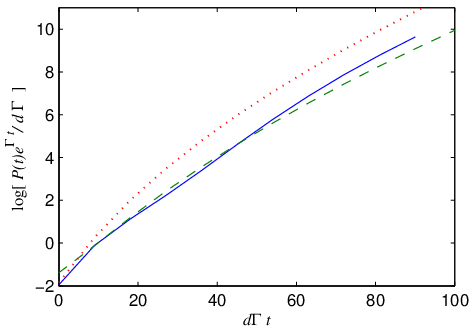
In Fig. 11 we analyze how the different corrections to the Raymer Mostowski calculation effects the total radiated power. We fix the Fresnel number at , as this is the limit where the Raymer Mostowski result is assumed to be valid. The curve is the simple result Eq. (VI.16). In curve we use the lowest order finite size correction, that is Eq. (VI.17). Finally in curve we use the general result from Eq. (VI.12), which is evaluated nummerically with the approximated Bessel function (VI.9). The approximation is used so that we gan get an estimation of the effect of all azimuthal quantum numbers, thus the nummerical methods require modest Fresnel numbers, such that the main contribution to the total radiated power comes from the mode coresponding to . We see that the simple Raymer Mostowski type result, Eq. (VI.16) over-estimates the total radiated power compared to the general result. We also see that the zeroth order result is a much better approximation in the regime .
Finally we compare the result of Eq. (VI.12) with a purely numerical calculation based on the point particle equations (II.21) and (II.22). To make such a comparison we need to connect the evolution of the atomic operators with the total intensity of the radiated field. Based on energy conservation, the evolution of the number of atoms in the ground state, is given by the number of photons exiting a boundary sphere enclosing the atomic ensemble. We derive this conservation law in Appendix D where we show that
| (VI.19) |
where is given by , and is given in Eq. (II.17). When comparing the result of Eq. (VI.12) to the atomic evolution we have to remember that we are only measuring half of the photons, since we only consider the emission at one end of the ensemble. Using that the evolution of the atomic operators are given by
| (VI.20) |
we find that the atomic operators evolve in time according to
| (VI.21) |
where we define as the matrix with elements given by . After taking quantum average of the result in Eq. (VI.19) we find that
| (VI.22) |
We then find the total intensity from the point particle model
| (VI.23) |
where we normalize with a factor since we want to compare the result with the result in Eq. (VI.12).
The advantages of making these calculations, or indeed solving the problem of SRS on a computer are clear. One avoids the problems of shifting from the point particle model to a continuous model. Thereby one also automatically include dipole dipole interaction effects connected to the point particle nature of the system which we have ignored here. Also the computer easily describes the total radiated field and not only the strongest super-radiating mode as we have analyzed here. On the other hand the direct method is numerically heavy for a large number of atoms, and we are limited to atoms. To understand the behavior at larger number of atoms it is therefore important to have an analytical theory along the lines considered here.
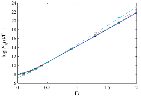
To make the numerical simulation we have randomly distributed between 3000 and 6000 atoms with a distribution function given by Eq. (III.2). After that the matrix is calculated and processed in order to find the total number of Stokes photons (VI.23). We can then by making a series of such realizations of the position of the atoms get some statistics on the inherent noise on the point particle model. In Fig. 12 we show the result of a numerical calculation using parameters and an optical depth of . When we increase the number of atoms, we decrease the particle density in order to keep a fixed Fresnel number and a fixed optical depth. We see from Fig. 12 that there is some dependence on particle density, an effect of the fact that the system is a point particle system and not a continuum, hence we do not expect the analytical theory developed so far to explain this effect. However as the density desceases the total radiated power converges.
Finally in Fig. 13 we compare the total radiated power in the analytical calculation , (VI.12), with the nummerical calculation , (VI.23). That the two methods gives very different results for small times is quite clear since initially the radiation is dominated by the spontaneous emission, which is not included in the analytical calculation. At increasing times, which is the regime where the analytical calculation is supposed to be valid, the two methods gives quite similar results, and we therefore believe that the analytical calculation gives an accurate description.
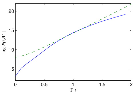
We finally note that for the time-scale used in Fig. 13, the approximation of neglecting depletion is not completely justified, as the number of emitted photons exceeds the number of atoms already before the two curves meet. We can examine the break-down of the no-depletion assumption, by finding the time , at which the number of photons emitted in the superradiating mode exceeds the number of atoms in the ensemble , i.e. , where
| (VI.24) |
To get an analytical result we will use the approximation , with given in Eq. (VI.17). After the integration in Eq. (VI.24) we find
| (VI.25) |
where we have used that . In Fig. 14 we plot the function . From the requirement we find the time for the result shown in Fig. 13 to be , where the radiation is still dominated by spontaneous emission. If, however we increase the optical depth we decrease the time at which the analytical curve , (VI.12), and the numerical curve , (VI.23), agree. For a higher optical depth there will thus be a region where the effects considered here are dominant within the applicability of our theory. While the limited atom number used here is thus not physically relevant, the simulation can still be used as a confirmation of the approximations used in our analytical calculation since both curves are derived using the same approximation of neglecting depletion of the atoms.

For the ongoing SRS experiments using Bose-Einstein condensed atoms e.g. Ref. [4] the number of atoms used in the process is factors of thousands larger than what we are able to numerically simulate here, and the approximation used here is much less severe.
VII Conclusion
In this paper we have developed a three-dimensional theory for spontaneous Raman scattering (SRS). The theory applies to an ensemble of non-moving atoms and is derived by describing the atoms as a continuous medium. In the theory we neglect the depletion of the initial atomic state and the theory is therefore mainly applicable to the onset and build up of SRS. We believe, however, that the theory still captures the most important effect of the three-dimensional structure of the problem, since after the onset of SRS the radiation is dominated by the modes determined by our theory.
The theory is based on a generalization of the one-dimensional theory in Ref. [11]. In the limit where the Fresnel is very large we find that the one-dimensional description of Ref. [11] applies to all transverse modes in agreement with the derivation in Ref. [9]. Without a detailed investigation of the three-dimensional structure there is, however, no restriction on the transverse momentum of the light and a naive application of the theory therefore predicts an infinite radiated intensity. In our three-dimensional theory the build up of SRS only happens for small transverse momentum of the light, limited by the Fresnel number of the ensemble. This automatically limits the emitted radiation such that the theory gives finite predictions.
In the theory we assume that the dimensions of the ensemble is much larger than the wavelength of the radiation, and we show that in this limit the only two parameters describing SRS are the optical depth and the Fresnel number of the ensemble. We find that in the limit the time scale of SRS is almost exclusively given by the optical depth with only a weak dependence on the Fresnel number . On the other hand, the total radiated power for SRS depends strongly on the Fresnel number . The total power radiated into modes with a given azimuthal quantum number is linearly proportional to . We find that the largest contribution to the radiation always comes from the azimuthal quantum number and that this contribution also have the fastest growth. With increasing Fresnel number the contribution from other azimuthal quantum numbers may, however, become comparable to the contribution. To investigate the validity of our analytical findings we have compared our analytical results to a direct numerical solution for a limited number of atoms. The two approaches are found to be in good agreement.
An interesting question which we have not addressed in detail here comes from the fact that an ensemble of atom is not given by a continuous density, but consists of a collection of discrete point particles. The effect of this is in principle included in our direct numerical investigations, and may be the reason for the dependence on the atom number in Fig. 12. Here the simulations with the highest density deviate from the results with a lower density. It would be interesting to investigate such effects using for instance the methods developed in Ref. [19]. Furthermore, the question of the collective emission of radiation from atomic ensembles is also very interesting from the point of view of quantum information. Several important quantum protocols such as quantum repeaters [26], quantum memory [27], and quantum teleportation [28] are currently being investigated in atomic ensembles. For a full evaluation of the potential of these approaches it will by important to have a full understanding of the effect of the realistic three dimensional structure of the ensembles. The methods developed in this article may serve as useful starting point for such investigations.
Acknowledgements.
We thank J.H. Müller, K. Mølmer and J. I. Cirac for usefull discussions. We acknowledge the financial support of the Future and Emerging Technologies (FET) programme within the Seventh Framework Programme for Research of the European Commission, under the FET-Open grant agreement HIDEAS, number FP7-ICT-221906.Appendix A Deriving the first order correction to the matrix
By introducing the dummy variable in the Gaussian function, the series expansion of the -integral in Eq. (IV.11) may be written as
| (A.1) |
Using the above expansion along with the relation together with the result [24]
| (A.2) |
Equation (A.1) may be rewritten as
| (A.3) |
From Ref. [24] we find the integral to give
| (A.4) |
We see that in terms of an expansion in the variable each differentiation will give a factor of . We shall therefore only consider a sum up to the first order in the differential. To zeroth order the -integral simply gives
| (A.5) |
To first order we find the -integral to give
| (A.6) |
To understand the above expression let us assume a sufficiently large so that the modified Bessel function can be approximated with . In this way we get
| (A.7) |
The above approximation gets worse for increasing values of , however we argue in Sec. VI.2, that for a finite width of the sample, higher order modes in has less influence. Finally the exponential function along with the modified Bessel function express a conservation of transverse momentum given by the variables since for increasing values of the transverse momentum, Eq. (A.7) can be approximated with
| (A.8) |
We shall then make the approximation
| (A.9) |
thus the expression in Eq. (A.8) can to second order in the difference be written as
| (A.10) |
This result is the large size limit, and we therefore conclude that to give this limit as the term in Eq. (A.6) must be approximated with
| (A.11) |
From this we conclude the result given in Eq. (IV.13).
Appendix B Commutation relation for and
Here we show that the two matrices and commute. Since both matrices are symmetric, it is enough to show that the product is symmetric. Again we make the continuation for . In this way we get
| (B.1) |
After making the -integral we end up with
| (B.2) |
Since the matrix Eq. (B.2) is symmetric we conclude that the matrices and commute.
Appendix C Derivation of Eq. (VI.11)
Here we will show Eq. (VI.11). Our starting point is the orthogonality relation given by
| (C.1) |
where the variable and is the ’th zero of the ’th order Bessel function . We will assume that is large, which does not require to be so, since we can choose the cut-off to be anything. In this way we can write Eq. (C.1) as
| (C.2) |
We will then take the sum over on both sides and use the standard continuation so that
| (C.3) |
Since is now a continuous variable, we conclude that the measure of the distribution
| (C.4) |
where is some real and positive number is unity. The next step is to show that for the function vanish. This follows when choosing a zero point and a cut-off such that say . This does not necessarily mean that has a similar representation with the chosen cut-off. On the other hand this is not necessary as one may show, see e.g. [21], that
| (C.5) |
from here we conclude that when and are different the function vanish. This concludes the derivation of Eq. (VI.11).
Appendix D The Sum rule
Here we derive the sum rule Eq. (VI.19) used in Sec. VI.3. The starting point is the total radiated intensity of Stokes-photons
| (D.1) |
where is a sphere surrounding the atoms. Using the Divergence theorem as well as the Maxwell equations, the total radiated intensity can be written as
| (D.2) | |||
| where | |||
| (D.3) | |||
To lowest order in , Eq. (D.2) reduce to
| (D.4) |
where we have used Eqs. (II.11), (II.17) and (II.18). When measuring the intensity infinitely far away from the atomic ensemble, the expression in Eq. (D.1) reduce to the electric field squared times , thus the normalized sum-rule reads
| (D.5) |
References
- [1] M. Gross, and S. Haroche, Phys. Rep. 93, 5, 301-396 (1982)
- [2] R. H. Dicke, Phys. Rev. 93, 1 (1954)
- [3] E. J. Woodbury and W. N. Ng, Proc. IRE 50, 2347 (1962)
- [4] A. Hilliard, F. Kaminski, R. le Targat, C. Olausson, E. S. Polzik, and J. H. Muller, Phys. Rev. A 78, 051403(R) (2008)
- [5] S. Inouye, A.P. Chikkatur, D. M. Stamper-Kurn, J. Stenger, D. E. Pritchard, and W. Ketterle, Science 285, 571 (1999)
- [6] D. Schneble, Y. Torii, M. Boyd, E. W. Streed, D. E. Pritchard, and W. Ketterle, Science 300, 475 (2003)
- [7] L. E. Sadler, J. M. Higbie, S.R. Leslie, M. Vengalattore, D. M. Stamper-Kurn, Phys. Rev. Lett. 98, 110401 (2007)
- [8] R. Bonifacio, C. Maroli, and N. Piovella, Opt. Commun. 68, 369 (1988)
- [9] K. Hammerer, A. S. Sørensen, and E. Polzik Quantum interface between light and atomic ensembles, arXiv:0807.3358v2
- [10] C. A. Muschik, E. S. Polzik, and J. I. Cirac, arXiv:0806.3448v2 [quant-ph] (2008)
- [11] M. G. Raymer, and J. Mostowski, Phys. Rev. A 24, 1980 (1981)
- [12] M. G. Raymer, I. A. Walmsley, J. Mostowski, and B. Sobolewska, Phys. Rev. A 32, 332 (1985)
- [13] M. G. Moore and P. Meystre, Phys. Rev. Lett. 83, 5202 (1999)
- [14] O. Zobay, and G. M. Nikolopoulos, Phys. Rev. A 72, 041604(R) (2005)
- [15] E. Akkermans, A. Gero, and R. Kaiser, Phys. Rev. Lett. 101, 103602 (2008)
- [16] L. H. Pedersen and Klaus Mølmer Few qubit atom-light interfaces with collective encoding, arXiv:0807.3610v2
- [17] D. Porras, and J. I. Cirac Collective generation of quantum states of light by entangled atoms, arXiv:0808.2732v1
- [18] A. A. Svidzinsky, J.-T. Chang, and M. O. Scully, Phys. Rev. Lett. 100, 160504 (2008)
- [19] M. W. Sorensen, and A. S. Sorensen, Phys. Rev. A 77, 013826 (2008)
- [20] I. E. Mazets and G. Kurizki, J. Phys. B 40, F105 (2007).
- [21] A. D. Jackson, Classical Electrodynamics, Third Edition (Wiley, New York, 1998).
- [22] O. Morice, Y. Castin, and J. Dalibard, Phys. Rev. A 51, 3896 (1995)
- [23] V.V.Klimov and M.Ducloy, Phys. Rev. A 69, 013812 (2004).
- [24] Gradshteyn and Ryzhik Tables of integrals, Series and Products, Academic Press (1965) .
- [25] G.N.Watson Theory of Bessel functions, Cambrige university press (1944).
- [26] L.-M. Duan, M. D. Lukin, J. I. Cirac and P. Zoller, Nature 414, 413 (2001).
- [27] B. Julsgaard, J. Sherson, J. I. Cirac, J. Fiurasek, and E. S. Polzik, Nature 432, 482 (2004).
- [28] J. F. Sherson, H. Krauter, R. K. Olsson, B. Julsgaard, K. Hammerer, J. I. Cirac, and E. S. Polzik, Nature 443, 557 (2006).