跳到论文正文
W Papers独立论文阅读器 arXiv:0903.0909 论文正文 计算阅读时间 · 0%
引用这篇论文根据当前论文元数据生成,正式投稿前建议核对。


License: arXiv.org perpetual non-exclusive license
arXiv:0903.0909v1 [math.PR] 05 Mar 2009

Optimal investment with counterparty risk:
a default-density modeling approach

Ying JIAO Affiliation: Laboratoire de Probabilités et Affiliation: Modèles Aléatoires Affiliation: CNRS, UMR 7599 Affiliation: Université Paris 7 Affiliation: e-mail: jiao@math.jussieu.fr    Huyên PHAM Affiliation: Laboratoire de Probabilités et Affiliation: Modèles Aléatoires Affiliation: CNRS, UMR 7599 Affiliation: Université Paris 7 Affiliation: e-mail: pham@math.jussieu.fr Affiliation: and Institut Universitaire de France
August 24, 2026
Abstract

We consider a financial market with a stock exposed to a counterparty risk inducing a drop in the price, and which can still be traded after this default time. We use a default-density modeling approach, and address in this incomplete market context the expected utility maximization from terminal wealth. We show how this problem can be suitably decomposed in two optimization problems in complete market framework: an after-default utility maximization and a global before-default optimization problem involving the former one. These two optimization problems are solved explicitly, respectively by duality and dynamic programming approaches, and provide a fine understanding of the optimal strategy. We give some numerical results illustrating the impact of counterparty risk and the loss given default on optimal trading strategies, in particular with respect to the Merton portfolio selection problem.

Key words: Counterparty risk, density of default time, optimal investment, duality, dynamic programming, backward stochastic differential equation.

1 Introduction

In a financial market, the default of a firm has usually important influences on the other ones. This has been shown clearly by several recent default events. The impact of a counterparty default may arise in various contexts. In terms of credit spreads, one observes in general a positive “jump” of the default intensity, called the contagious jump and investigated firstly by Jarrow and Yu [5]. In terms of asset (or stock) values for a firm, the default of a counterparty will in general induce a drop of its value process. In this paper, we analyze the impact of this risk on the optimal investment problem. More precisely, we consider an agent, who invests in a risky asset exposed to a counterparty risk, and we are interested in the optimal trading strategy and the value function when taking into account the possibility of default of a counterparty, together with the instantaneous loss of the asset at the default time.

The global market information containing default is modeled by the progressive enlargement of a background filtration, denoted by 𝔽\mathbb{F}, representing the default-free information. The default time τ\tau is in general a totally inaccessible stopping time with respect to the enlarged filtration, but is not an 𝔽\mathbb{F}-stopping time. We shall work with a density hypothesis of the conditional law of default given 𝔽\mathbb{F}. This hypothesis has been introduced by Jacod [4] in the initial enlargement of filtrations, and has been adopted recently by El Karoui et al. [3] in the progressive enlargement setting for the credit risk analysis. The density approach is particularly suitable to study what goes on after the default, i.e., on {τ≤t}\{\tau\leq t\}. For the before-default analysis on {τ>t}\{\tau>t\}, there exists an explicit relationship between the density approach and the widely used intensity approach.

The market model considered here is incomplete due to the jump induced by the default time. The general optimal investment problem in an incomplete market has been studied by Kramkov and Schachermayer [7] by duality methods. Recently, Lim and Quenez [8] addressed, by using dynamic programming, the utility maximization in a market with default. The key idea of our paper is to derive, by relying on the conditional density approach of default, a natural separation of the initial optimization problem into an after-default one and a global before-default one. Both problems are reduced to a complete market setting, and the solution of the latter one depends on the solution of the former one. These two optimization problems are solved by duality and dynamic programming approaches, and the main advantage is to give a better insight, and more explicit results than the incomplete market framework. The interesting feature of our decomposition is to provide a nice interpretation of optimal strategy switching at the default time τ\tau. Moreover, the explicit solution (for the CRRA utility function) makes clear the roles played by the default time τ\tau and the loss given default in the investment strategy, as shown by some numerical examples.

The outline of this article is organized as follows. In Section 2, we present the model and the investment problem, and introduce the default density hypothesis. We then explain in Section 3 how to decompose the optimal investment problem into the before-default and after-default ones. We solve these two optimization problems in Section 4, by using the duality approach for the after-default one and the dynamic programming approach for the global before-default one. We examine more in detail the popular case of CRRA utility function and finally, numerical results illustrate the impact of counterparty risk on optimal trading strategies, in particular with respect to the classical Merton portfolio selection problem.

2 The conditional density model for counterparty risk

We consider a financial market model with a riskless bond assumed for simplicity equal to one, and a stock subject to a counterparty risk: the dynamics of the risky asset is affected by another firm, the counterparty, which may default, inducing consequently a drop in the asset price. However, this stock still exists and can be traded after the default of the counterparty.

Let us fix a probability space (Ω,𝒢,ℙ)(\Omega,{\cal G},\mathbb{P}) equipped with a brownian motion WW == (Wt)t∈[0,T](W_{t})_{t\in[0,T]} over a finite horizon TT << ∞\infty, and denote by 𝔽\mathbb{F} == (ℱt)t∈[0,T]({\cal F}_{t})_{t\in[0,T]} the natural filtration of WW. We are given a nonnegative and finite random variable τ\tau, representing the default time, on (Ω,𝒢,ℙ)(\Omega,{\cal G},\mathbb{P}). Before the default time τ\tau, the filtration 𝔽\mathbb{F} represents the information accessible to the investors. When the default occurs, the investors add this new information τ\tau to the reference filtration 𝔽\mathbb{F}. We then introduce DtD_{t} == 1τ≤t1_{\tau\leq t}, 0≤t≤T0\leq t\leq T, 𝔻\mathbb{D} == (𝒟t)t∈[0,T]({\cal D}_{t})_{t\in[0,T]} the filtration generated by this jump process, and 𝔾\mathbb{G} == (𝒢t)t∈[0,T]({\cal G}_{t})_{t\in[0,T]} the enlarged progressive filtration 𝔽∨𝔻\mathbb{F}\vee\mathbb{D}, representing the structure of information available for the investors over [0,T][0,T].

The stock price process is governed by the dynamics:

d​St\displaystyle dS_{t} =\displaystyle= St−​(μt​d​t+σt​d​Wt−γt​d​Dt),     0≤t≤T,\displaystyle S_{t-}\big(\mu_{t}dt+\sigma_{t}dW_{t}-\gamma_{t}dD_{t}\big),\;\;\;\;\;0\leq t\leq T, (2.1)

where μ\mu, σ\sigma and γ\gamma are 𝔾\mathbb{G}-predictable processes. At this stage, without any further condition on the default time τ\tau, we do not know yet that WW is a 𝔾\mathbb{G}-semimartingale (see Remark 2.1), and the meaning of the sde (2.1) is the following. Recall (cf. [9]) that any 𝔾\mathbb{G}-predictable process φ\varphi can be written in the form: φt\varphi_{t} == φt𝔽​1t≤τ\varphi_{t}^{\mathbb{F}}1_{t\leq\tau} ++ φtd​(τ)​1t>τ\varphi_{t}^{d}(\tau)1_{t>\tau}, 0≤t≤T0\leq t\leq T, where φ𝔽\varphi^{\mathbb{F}} is 𝔽\mathbb{F}-adapted, and φtd​(θ)\varphi_{t}^{d}(\theta) is measurable w.r.t. ℱt⊗ℬ⁡(ℝ+){\cal F}_{t}\otimes\mathcal{B}(\mathbb{R}_{+}), for all tt ∈\in [0,T][0,T]. The dynamics (2.1) is then written as:

d​St\displaystyle dS_{t} =\displaystyle= St​(μt𝔽​d​t+σt𝔽​d​Wt),     0≤t<τ,\displaystyle S_{t}\big(\mu_{t}^{\mathbb{F}}dt+\sigma_{t}^{\mathbb{F}}dW_{t}\big),\;\;\;\;\;0\leq t<\tau, (2.2)
Sτ\displaystyle S_{\tau} =\displaystyle= Sτ−​(1−γτ𝔽),\displaystyle S_{\tau^{-}}(1-\gamma_{\tau}^{\mathbb{F}}), (2.3)
d​St\displaystyle dS_{t} =\displaystyle= St​(μtd​(τ)​d​t+σtd​(τ)​d​Wt),τ<t≤T,\displaystyle S_{t}\big(\mu_{t}^{d}(\tau)dt+\sigma_{t}^{d}(\tau)dW_{t}\big),\;\;\;\;\;\tau<t\leq T, (2.4)

where μ𝔽\mu^{\mathbb{F}}, σ𝔽\sigma^{\mathbb{F}}, γ𝔽\gamma^{\mathbb{F}} are 𝔽\mathbb{F}-adapted processes, and (ω,θ)(\omega,\theta) →\rightarrow μtd​(θ)\mu_{t}^{d}(\theta), σtd​(θ)\sigma_{t}^{d}(\theta) are ℱt⊗ℬ⁡([0,t)){\cal F}_{t}\otimes\mathcal{B}([0,t))-measurables functions for all tt ∈\in [0,T][0,T]. The nonnegative process γ\gamma represents the (proportional) loss on the stock price induced by the default of the counterparty, and we may assume that γ\gamma is a stopped process at τ\tau, i.e. γt\gamma_{t} == γt∧τ\gamma_{t\wedge\tau}. By misuse of notation, we shall thus identify γ\gamma in (2.1) with the 𝔽\mathbb{F}-adapted process γ𝔽\gamma^{\mathbb{F}} in (2.3). When the counterparty defaults, the drift and diffusion coefficients (μ,σ)(\mu,\sigma) of the stock price switch from (μ𝔽CLOSE(\mu^{\mathbb{F}},OPENσ𝔽)\sigma^{\mathbb{F}}) to (μd​(τ),σd​(τ))(\mu^{d}(\tau),\sigma^{d}(\tau)), and the after-default coefficients may depend on the default time τ\tau. We assume that σt\sigma_{t} >> 00, 0≤t≤T0\leq t\leq T, the following integrability conditions are satisfied:

∫0T|μtσt|2​𝑑t+∫0T|σt|2​𝑑t\displaystyle\int_{0}^{T}\Big|\frac{\mu_{t}}{\sigma_{t}}\Big|^{2}dt+\int_{0}^{T}|\sigma_{t}|^{2}dt <\displaystyle< ∞,a.s.\displaystyle\infty,\;\;\;\;a.s. (2.5)

and

0≤γt\displaystyle 0\leq\gamma_{t} <\displaystyle< 1,   0≤t≤T,a.s.\displaystyle 1,\;\;\;0\leq t\leq T,\;\;\;a.s. (2.6)

which ensure that the dynamics of the asset price process is well-defined, and the stock price remains (strictly) positive over [0,T][0,T] (once the initial stock price S0S_{0} >> 00), and locally bounded.

Consider now an investor who can trade continuously in this financial market by holding a positive wealth at any time. This is mathematically quantified by a 𝔾\mathbb{G}-predictable process π\pi == (πt)t∈[0,T](\pi_{t})_{t\in[0,T]}, called trading strategy and representing the proportion of wealth invested in the stock, and the associated wealth process XX with dynamics:

d​Xt\displaystyle dX_{t} =\displaystyle= πt​Xt−​d​StSt−,     0≤t≤T.\displaystyle\pi_{t}X_{t^{-}}\frac{dS_{t}}{S_{t-}},\;\;\;\;\;0\leq t\leq T. (2.7)

By writing the 𝔾\mathbb{G}-predictable process π\pi in the form: πt\pi_{t} == πt𝔽​1t≤τ\pi_{t}^{\mathbb{F}}1_{t\leq\tau} ++ πtd​(τ)​1t>τ\pi_{t}^{d}(\tau)1_{t>\tau}, 0≤t≤T0\leq t\leq T, where π𝔽\pi^{\mathbb{F}} is 𝔽\mathbb{F}-adapted and πtd​(θ)\pi_{t}^{d}(\theta) is ℱt⊗ℬ⁡([0,t)){\cal F}_{t}\otimes\mathcal{B}([0,t))-measurable, and in view of (2.2)-(2.3)-(2.4), the wealth process evolves as

d​Xt\displaystyle dX_{t} =\displaystyle= Xt​πt𝔽​(μt𝔽​d​t+σt𝔽​d​Wt),     0≤t<τ,\displaystyle X_{t}\pi_{t}^{\mathbb{F}}\big(\mu_{t}^{\mathbb{F}}dt+\sigma_{t}^{\mathbb{F}}dW_{t}\big),\;\;\;\;\;0\leq t<\tau, (2.8)
Xτ\displaystyle X_{\tau} =\displaystyle= Xτ−​(1−πτ𝔽​γτ)\displaystyle X_{\tau^{-}}(1-\pi_{\tau}^{\mathbb{F}}\gamma_{\tau}) (2.9)
d​Xt\displaystyle dX_{t} =\displaystyle= Xt​πtd​(τ)​(μtd​(τ)​d​t+σtd​(τ)​d​Wt),τ<t≤T.\displaystyle X_{t}\pi_{t}^{d}(\tau)\big(\mu_{t}^{d}(\tau)dt+\sigma_{t}^{d}(\tau)dW_{t}\big),\;\;\;\;\;\tau<t\leq T. (2.10)

We say that a trading strategy π\pi is admissible, and we denote π\pi ∈\in 𝒜{\cal A}, if

∫0T|πt​σt|2​𝑑t<∞,\displaystyle\int_{0}^{T}|\pi_{t}\sigma_{t}|^{2}dt\;<\;\infty, and πτ​γτ<1​a.s.\displaystyle\pi_{\tau}\gamma_{\tau}<1\;\;\;a.s.

This ensures that the dynamics of the wealth process is well-defined with a positive wealth at any time (once starting from a positive initial capital X0X_{0} >> 00).

In the sequel, we shall make the standing assumption, called density hypothesis, on the default time of the counterparty. For any tt ∈\in [0,T][0,T], the conditional distribution of τ\tau given ℱt{\cal F}_{t} admits a density with respect to the Lebesgue measure, i.e. there exists a family of ℱt⊗ℬ⁡(ℝ+)\mathcal{F}_{t}\otimes\mathcal{B}(\mathbb{R}_{+})-measurable positive functions (ω,θ)(\omega,\theta) →\rightarrow αt​(θ)\alpha_{t}(\theta) such that:

(𝐃𝐇)ℙ⁡[τ∈d​θ|ℱt]\displaystyle\hskip-85.35826pt{\bf(DH)}\hskip 113.81102pt\mathbb{P}[\tau\in d\theta|\mathcal{F}_{t}] =\displaystyle= αt​(θ)​d​θ,t∈[0,T].\displaystyle\alpha_{t}(\theta)d\theta,\;\;\;\;\;t\in[0,T].

We note that for any θ≥0\theta\geq 0, the process {αt(θ),0≤t≤T}\{\alpha_{t}(\theta),0\leq t\leq T\} is a (ℙ,𝔽)(\mathbb{P},\mathbb{F})-martingale.

Remark 2.1

Such a hypothesis is usual in the theory of initial enlargement of filtration, and was introduced by Jacod [4]. The (DH) Hypothesis was recently adopted by El Karoui et al. [3] in the progressive enlargement of filtration for credit risk modeling. Notice that in the particular case where the family of densities satisfies αT​(t)\alpha_{T}(t) == αt​(t)\alpha_{t}(t) for all 0≤t≤T0\leq t\leq T, we have ℙ⁡[τ>t|ℱt]\mathbb{P}[\tau>t|\mathcal{F}_{t}] == ℙ⁡[τ>t|ℱT]\mathbb{P}[\tau>t|\mathcal{F}_{T}]. This corresponds to the so-called immersion hypothesis (or the H-hypothesis), which is a familiar condition in credit risk analysis, and means equivalently that any square-integrable 𝔽\mathbb{F}-martingale is a square-integrable 𝔾\mathbb{G}-martingale. The H-hypothesis appears natural for the analysis on before-default events when t<τt<\tau, but is actually restrictive when it concerns after-default events on {t≥τ}\{t\geq\tau\}, see [3] for a more detailed discussion. By considering here the whole family {αt​(θ),t∈[0,T],θ∈ℝ+}\{\alpha_{t}(\theta),t\in[0,T],\theta\in\mathbb{R}_{+}\}, we obtain additional information for the analysis of after-default events, which is crucial for our purpose.

Let us also mention that the classical intensity of default can be expressed in an explicit way by means of the density. Indeed, the (ℙ,𝔾)(\mathbb{P},\mathbb{G})-predictable compensator of DtD_{t} == 1τ≤t1_{\tau\leq t} is given by ∫0t∧ταθ​(θ)/Gθ​𝑑θ\int_{0}^{t\wedge\tau}\alpha_{\theta}(\theta)/G_{\theta}d\theta, where GtG_{t} == ℙ⁡[τ>t|ℱt]\mathbb{P}[\tau>t|\mathcal{F}_{t}] is the conditional survival probability. In other words, the process MtM_{t} == Dt−∫0t∧ταθ​(θ)/Gθ​𝑑θD_{t}-\int_{0}^{t\wedge\tau}\alpha_{\theta}(\theta)/G_{\theta}d\theta is a (ℙ,𝔾)(\mathbb{P},\mathbb{G})-martingale. Thus, by observing from the martingale property of {αt(θ),0≤t≤T}\{\alpha_{t}(\theta),0\leq t\leq T\} that GtG_{t} == ∫t∞αt​(θ)​𝑑θ\int_{t}^{\infty}\alpha_{t}(\theta)d\theta == ∫t∞𝔼⁡[αθ​(θ)|ℱt]​𝑑θ\int_{t}^{\infty}\mathbb{E}[\alpha_{\theta}(\theta)|\mathcal{F}_{t}]d\theta, we recover completely the intensity process λt𝔾\lambda_{t}^{\mathbb{G}} == 1t≤τ​αt​(t)/Gt1_{t\leq\tau}\,\alpha_{t}(t)/G_{t} from the knowledge of the process {αt​(t),t≥0}\{\alpha_{t}(t),t\geq 0\}. However, given the intensity λ𝔾\lambda^{\mathbb{G}}, we can only obtain some part of the density family, namely αt​(θ)\alpha_{t}(\theta) for θ≥t\theta\geq t.

Under (DH) Hypothesis, a (ℙ,𝔽)(\mathbb{P},\mathbb{F})-brownian motion WW is a 𝔾\mathbb{G}-semimartingale and admits an explicit decomposition in terms of the density α\alpha given by (see [9], [6], [3]):

Wt\displaystyle W_{t} =\displaystyle= W^t𝔾+∫0t∧τd​⟨Ws,Gs⟩Gs+∫τtd⁡⟨Ws,αs​(τ)⟩αs​(τ)=:W^t𝔾+At,   0≤t≤T,\displaystyle\hat{W}_{t}^{\mathbb{G}}+\int_{0}^{t\wedge\tau}\frac{d\left<W_{s},G_{s}\right>}{G_{s}}+\int_{\tau}^{t}\frac{d\left<W_{s},\alpha_{s}(\tau)\right>}{\alpha_{s}(\tau)}\;=:\;\hat{W}_{t}^{\mathbb{G}}+A_{t},\;\;\;0\leq t\leq T,

where W^𝔾\hat{W}^{\mathbb{G}} is a (ℙ,𝔾)(\mathbb{P},\mathbb{G})-brownian motion, and AA is a finite variation 𝔾\mathbb{G}-adapted process. Moreover, by the Itô martingale representation theorem for brownian filtration 𝔽\mathbb{F}, AtA_{t} is written in the form AtA_{t} == ∫0tas​𝑑s\int_{0}^{t}a_{s}ds for some 𝔾\mathbb{G}-adapted process aa == (at)t∈[0,T](a_{t})_{t\in[0,T]}. Let us then define the 𝔾\mathbb{G}-adapted process

βt\displaystyle\beta_{t} =\displaystyle= μt+σt​at−γt​λt𝔾σt,   0≤t≤T,\displaystyle\frac{\mu_{t}+\sigma_{t}a_{t}-\gamma_{t}\lambda_{t}^{\mathbb{G}}}{\sigma_{t}},\;\;\;0\leq t\leq T,

and consider the Doléans-Dade exponential local martingale: Zt𝔾Z_{t}^{\mathbb{G}} == ℰ(−∫βdW^𝔾)t{\cal E}(-\int\beta d\hat{W}^{\mathbb{G}})_{t}, 0≤t≤T0\leq t\leq T. By assuming that Z𝔾Z^{\mathbb{G}} is a (ℙ,𝔾)(\mathbb{P},\mathbb{G})-martingale (which is satisfied e.g. under the Novikov criterion: 𝔼⁡[exp⁡(∫0T12​|βt|2​𝑑t)]\mathbb{E}[\exp(\int_{0}^{T}\frac{1}{2}|\beta_{t}|^{2}dt)] << ∞\infty), this defines a probability measure ℚ\mathbb{Q} equivalent to ℙ\mathbb{P} on (Ω,𝒢T)(\Omega,{\cal G}_{T}) with Radon-Nikodym density:

d​ℚd​ℙ\displaystyle\frac{d\mathbb{Q}}{d\mathbb{P}} =\displaystyle= ZT𝔾=exp(−∫0TβtdW^t𝔾−12∫0T|βt|2dt),\displaystyle Z_{T}^{\mathbb{G}}\;=\;\exp\Big(-\int_{0}^{T}\beta_{t}d\hat{W}_{t}^{\mathbb{G}}-\frac{1}{2}\int_{0}^{T}|\beta_{t}|^{2}dt\Big),

under which, by Girsanov’s theorem (see [1] Ch.5.2), W¯𝔾\overline{W}^{\mathbb{G}} == W^𝔾+∫β​𝑑t\hat{W}^{\mathbb{G}}+\int\beta dt is a (ℚ,𝔾)(\mathbb{Q},\mathbb{G})-Brownian motion, MM is a (ℚ,𝔾)(\mathbb{Q},\mathbb{G})-martingale, so that the dynamics of SS follows a (ℚ,𝔾)(\mathbb{Q},\mathbb{G})-local martingale:

d​St\displaystyle dS_{t} =\displaystyle= St−​(σt​d​W¯t𝔾−γt​d​Mt).\displaystyle S_{t^{-}}(\sigma_{t}d\overline{W}_{t}^{\mathbb{G}}-\gamma_{t}dM_{t}).

We thus have the “no-arbitrage” condition

ℳ⁡(𝔾)\displaystyle{\cal M}(\mathbb{G}) :⁣=\displaystyle:= {ℚ∼ℙ​ on ​(Ω,𝒢T):S​ is a ​(ℚ,𝔾)−local martingale}≠∅.\displaystyle\{\mathbb{Q}\sim\mathbb{P}\mbox{ on }(\Omega,{\cal G}_{T}):S\mbox{ is a }(\mathbb{Q},\mathbb{G})-\mbox{local martingale}\}\;\neq\;\emptyset. (2.11)

3 Decomposition of the utility maximization problem

We are given an utility function UU defined on (0,∞)(0,\infty), strictly increasing, strictly concave and C1C^{1} on (0,∞)(0,\infty), and satisfying the Inada conditions U′​(0+)U^{\prime}(0^{+}) == ∞\infty, U′​(∞)U^{\prime}(\infty) == 00. The performance of an admissible trading strategy π\pi ∈\in 𝒜{\cal A} associated to a wealth process XX solution to (2.7) and starting at time 00 from X0X_{0} >> 00, is measured over the finite horizon TT by:

J0​(π)\displaystyle J_{0}(\pi) =\displaystyle= 𝔼⁡[U⁡(XT)],\displaystyle\mathbb{E}[U(X_{T})],

and the optimal investment problem is formulated as:

V0\displaystyle V_{0} =\displaystyle= supπ∈𝒜J0​(π).\displaystyle\sup_{\pi\in{\cal A}}J_{0}(\pi). (3.1)

Problem (3.1) is a maximization problem of expected utility from terminal wealth in an incomplete market due to the jump of the risky asset. This optimization problem can be studied by convex duality methods. Actually, under the condition that

V0\displaystyle V_{0} <\displaystyle< ∞,\displaystyle\infty, (3.2)

which is satisfied under (2.11) once

𝔼​[U~​(y​d​ℚd​ℙ)]\displaystyle\mathbb{E}\Big[\tilde{U}\big(y\frac{d\mathbb{Q}}{d\mathbb{P}}\big)\Big] <\displaystyle< ∞, for some ​y>0,\displaystyle\infty,\;\;\;\mbox{ for some }y>0,

where U~​(y)\tilde{U}(y) == supx>0[U⁡(x)−x​y]\sup_{x>0}[U(x)-xy], and under the so-called condition of reasonable asymptotic elasticity:

A​E​(U):=lim supx→∞x​U′​(x)U⁡(x)< 1,\displaystyle AE(U):=\limsup_{x\rightarrow\infty}\frac{xU^{\prime}(x)}{U(x)}\;<\;1,

we know from the general results of Kramkov and Schachermayer [7] that there exists a solution to (3.1). We also have a dual characterization of the solution, but this does not lead to explicit results due to the incompleteness of the market, i.e. the infinite cardinality of ℳ⁡(𝔾){\cal M}(\mathbb{G}). One can also deal with problem (3.1) by dynamic programming methods as done recently in Lim and Quenez [8] under (H) hypothesis, but again, except for the logarithmic utility function, this does not yield explicit characterization of the optimal strategy. We provide here an alternative approach by making use of the specific feature of the jump of the stock induced by the default time under the density hypothesis. The main idea is to separate the problem in two portfolio optimization problems in complete markets: the after-default and before-default maximization problems. This gives a better understanding of the optimal strategy and allows us to derive explicit results in some particular cases of interest.

The derivation starts as follows. First notice that any π\pi ∈\in 𝒜{\cal A}, thus in the form: πt\pi_{t} == πt𝔽​1t≤τ\pi_{t}^{\mathbb{F}}1_{t\leq\tau} ++ πtd​(τ)​1t>τ\pi_{t}^{d}(\tau)1_{t>\tau}, 0≤t≤T0\leq t\leq T, can be identified with a pair (π𝔽,πd)(\pi^{\mathbb{F}},\pi^{d}) ∈\in 𝒜𝔽×𝒜d{\cal A}_{\mathbb{F}}\times{\cal A}_{d} where 𝒜𝔽{\cal A}_{\mathbb{F}} is the set of admissible trading strategies in absence of defaults, i.e. the set of 𝔽\mathbb{F}-adapted processes π𝔽\pi^{\mathbb{F}} s.t.

∫0T|πt𝔽​σt𝔽|2​𝑑t<∞,\displaystyle\int_{0}^{T}|\pi_{t}^{\mathbb{F}}\sigma_{t}^{\mathbb{F}}|^{2}dt\;<\;\infty, and πθγθ<1,   0≤θ≤T,a.s.\displaystyle\pi_{\theta}\gamma_{\theta}<1,\;\;\;0\leq\theta\leq T,\;a.s. (3.3)

and 𝒜d{\cal A}_{d} is the set of admissible trading strategies after default at time τ\tau == θ\theta, i.e. the set of Borel family of 𝔽\mathbb{F}-adapted processes {πtd(θ),θ<t≤T}\{\pi^{d}_{t}(\theta),\theta<t\leq T\} parametrized by θ\theta ∈\in [0,T][0,T] s.t.

∫θT|πtd​(θ)​σtd​(θ)|2​𝑑t\displaystyle\int_{\theta}^{T}|\pi_{t}^{d}(\theta)\sigma_{t}^{d}(\theta)|^{2}dt <\displaystyle< ∞,a.s.\displaystyle\infty,\;\;\;\;\;a.s.

Hence, for any π\pi == (π𝔽,πd)(\pi^{\mathbb{F}},\pi^{d}) ∈\in 𝒜{\cal A}, we observe by (2.8)-(2.9)-(2.10) that the terminal wealth is written as:

XT\displaystyle X_{T} =\displaystyle= XT𝔽​1τ>T+XTd​(τ)​1τ≤T,\displaystyle X_{T}^{\mathbb{F}}1_{\tau>T}+X_{T}^{d}(\tau)1_{\tau\leq T},

where X𝔽X^{\mathbb{F}} is the wealth process in absence of default, governed by:

d​Xt𝔽\displaystyle dX_{t}^{\mathbb{F}} =\displaystyle= Xt𝔽​πt𝔽​(μt𝔽​d​t+σt𝔽​d​Wt),     0≤t≤T,\displaystyle X_{t}^{\mathbb{F}}\pi_{t}^{\mathbb{F}}\big(\mu_{t}^{\mathbb{F}}dt+\sigma_{t}^{\mathbb{F}}dW_{t}\big),\;\;\;\;\;0\leq t\leq T, (3.4)

starting from X0𝔽X_{0}^{\mathbb{F}} == X0X_{0}, and {Xtd(θ),θ≤t≤T}\{X_{t}^{d}(\theta),\theta\leq t\leq T\} is the wealth process after default occuring at τ\tau == θ∈[0,T]\theta\in[0,T], governed by:

d​Xtd​(θ)\displaystyle dX_{t}^{d}(\theta) =\displaystyle= Xtd​(θ)​πtd​(θ)​(μtd​(θ)​d​t+σtd​(θ)​d​Wt),θ<t≤T\displaystyle X_{t}^{d}(\theta)\pi_{t}^{d}(\theta)\big(\mu_{t}^{d}(\theta)dt+\sigma_{t}^{d}(\theta)dW_{t}\big),\;\;\;\;\;\theta<t\leq T (3.5)
Xθd​(θ)\displaystyle X_{\theta}^{d}(\theta) =\displaystyle= Xθ𝔽​(1−πθ𝔽​γθ).\displaystyle X_{\theta}^{\mathbb{F}}(1-\pi_{\theta}^{\mathbb{F}}\gamma_{\theta}). (3.6)

Therefore, under the density hypothesis (DH), and by the law of iterated conditional expectations, the performance measure may be written as:

J0​(π)\displaystyle J_{0}(\pi) =\displaystyle= 𝔼⁡[𝔼⁡[U⁡(XT)|ℱT]]=𝔼⁡[U⁡(XT𝔽)​ℙ​[τ>T|ℱT]+𝔼⁡[U⁡(XTd​(τ))​1τ≤T|ℱT]]\displaystyle\mathbb{E}\big[\mathbb{E}[U(X_{T})|{\cal F}_{T}]\big]\;=\;\mathbb{E}\big[U(X_{T}^{\mathbb{F}})\mathbb{P}[\tau>T|{\cal F}_{T}]+\mathbb{E}[U(X_{T}^{d}(\tau))1_{\tau\leq T}|{\cal F}_{T}]\big] (3.7)
=\displaystyle= 𝔼⁡[U⁡(XT𝔽)​GT+∫0TU⁡(XTd​(θ))​αT​(θ)​𝑑θ],\displaystyle\mathbb{E}\Big[U(X_{T}^{\mathbb{F}})G_{T}+\int_{0}^{T}U(X_{T}^{d}(\theta))\alpha_{T}(\theta)d\theta\Big],

where GTG_{T} == ℙ⁡[τ>T|ℱT]\mathbb{P}[\tau>T|{\cal F}_{T}] == ∫T∞αT​(θ)​𝑑θ\int_{T}^{\infty}\alpha_{T}(\theta)d\theta.

Let us introduce the value-function process of the “after-default” optimization problem:

Vθd​(x)\displaystyle V^{d}_{\theta}(x) =\displaystyle= ess​supπd​(θ)∈𝒜d​(θ)​Jθd​(x,πd​(θ)),(θ,x)∈[0,T]×(0,∞),\displaystyle\underset{\pi^{d}(\theta)\in{\cal A}_{d}(\theta)}{\mathrm{ess\,sup\,}}J^{d}_{\theta}(x,\pi^{d}(\theta)),\;\;(\theta,x)\in[0,T]\times(0,\infty), (3.8)
Jθd​(x,πd​(θ))\displaystyle J^{d}_{\theta}(x,\pi^{d}(\theta)) =\displaystyle= 𝔼⁡[U⁡(XTd,x​(θ))​αT​(θ)|ℱθ],\displaystyle\mathbb{E}\big[U(X_{T}^{d,x}(\theta))\alpha_{T}(\theta)\big|{\cal F}_{\theta}\big],

where 𝒜d​(θ){\cal A}_{d}(\theta) is the set of (ℱt)θ<t≤T({\cal F}_{t})_{\theta<t\leq T}-adapted processes {πtd(θ),θ<t≤T}\{\pi^{d}_{t}(\theta),\theta<t\leq T\} satisfying ∫θT|πtd​(θ)​σtd​(θ)|2​𝑑t\int_{\theta}^{T}|\pi_{t}^{d}(\theta)\sigma_{t}^{d}(\theta)|^{2}dt << ∞\infty a.s., and {Xtd,x(θ),θ≤t≤T}\{X_{t}^{d,x}(\theta),\theta\leq t\leq T\} is the solution to (3.5) controlled by πd​(θ)\pi^{d}(\theta) ∈\in 𝒜d​(θ){\cal A}_{d}(\theta), starting from xx at time θ\theta. Thus, VdV^{d} is the value-function process of an optimal investment problem in a market model after default. Notice that the coefficients (μd,σd)(\mu^{d},\sigma^{d}) of the model depend on the initial time θ\theta when the maximization is performed, and the utility function in the criterion is weighted by αT​(θ)\alpha_{T}(\theta). We shall see in the next section how to deal with these peculiarities for solving (3.8) and proving the existence and characterization of an optimal strategy.

The main result of this section is to show that the original problem (3.1) can be split into the above after-default optimization problem, and a global optimization problem in a before-default market.

Theorem 3.1

Assume that Vθd​(x)V_{\theta}^{d}(x) << ∞\infty a.s. for all (θ,x)∈[0,T]×(0,∞)(\theta,x)\in[0,T]\times(0,\infty). Then, we have:

V0\displaystyle V_{0} =\displaystyle= supπ𝔽∈𝒜𝔽𝔼⁡[U⁡(XT𝔽)​GT+∫0TVθd​(Xθ𝔽​(1−πθ𝔽​γθ))​𝑑θ].\displaystyle\sup_{\pi^{\mathbb{F}}\in{\cal A}_{\mathbb{F}}}\mathbb{E}\Big[U(X_{T}^{\mathbb{F}})G_{T}+\int_{0}^{T}V^{d}_{\theta}(X_{\theta}^{\mathbb{F}}(1-\pi_{\theta}^{\mathbb{F}}\gamma_{\theta}))d\theta\Big]. (3.9)

Proof. Given π\pi == (π𝔽,πd)(\pi^{\mathbb{F}},\pi^{d}) ∈\in 𝒜{\cal A}, we have the relation (3.7) for J0​(π)J_{0}(\pi) under (DH). Furthermore, by Fubini’s theorem, the law of iterated conditional expectations, we then obtain:

J0​(π)\displaystyle J_{0}(\pi) =\displaystyle= 𝔼⁡[U⁡(XT𝔽)​GT+∫0T𝔼⁡[U⁡(XTd​(θ))​αT​(θ)|ℱθ]​𝑑θ]\displaystyle\mathbb{E}\Big[U(X_{T}^{\mathbb{F}})G_{T}+\int_{0}^{T}\mathbb{E}\big[U(X_{T}^{d}(\theta))\alpha_{T}(\theta)\big|{\cal F}_{\theta}]d\theta\Big] (3.10)
=\displaystyle= 𝔼⁡[U⁡(XT𝔽)​GT+∫0TJθd​(Xθd​(θ),πd​(θ))​𝑑θ]\displaystyle\mathbb{E}\Big[U(X_{T}^{\mathbb{F}})G_{T}+\int_{0}^{T}J^{d}_{\theta}(X_{\theta}^{d}(\theta),\pi^{d}(\theta))d\theta\Big]
≤\displaystyle\leq 𝔼⁡[U⁡(XT𝔽)​GT+∫0TVθd​(Xθd​(θ))​𝑑θ]\displaystyle\mathbb{E}\Big[U(X_{T}^{\mathbb{F}})G_{T}+\int_{0}^{T}V^{d}_{\theta}(X_{\theta}^{d}(\theta))d\theta\Big]
≤\displaystyle\leq supπ𝔽∈𝒜𝔽𝔼⁡[U⁡(XT𝔽)​GT+∫0TVθd​(Xθ𝔽​(1−πθ𝔽​γθ))​𝑑θ]=:V^0.\displaystyle\sup_{\pi^{\mathbb{F}}\in{\cal A}_{\mathbb{F}}}\mathbb{E}\Big[U(X_{T}^{\mathbb{F}})G_{T}+\int_{0}^{T}V^{d}_{\theta}(X_{\theta}^{\mathbb{F}}(1-\pi_{\theta}^{\mathbb{F}}\gamma_{\theta}))d\theta\Big]=:\hat{V}_{0}.

by definitions of JdJ^{d}, VdV^{d} and Xθd​(θ)X_{\theta}^{d}(\theta). This proves the inequality: V0V_{0} ≤\leq V^0\hat{V}_{0}.

To prove the converse inequality, fix an arbitrary π𝔽\pi^{\mathbb{F}} ∈\in 𝒜𝔽{\cal A}_{\mathbb{F}}. By definition of VdV^{d}, for any ω\omega ∈\in Ω\Omega, θ\theta ∈\in [0,T][0,T], and ε\varepsilon >> 00, there exists πd,ε,ω​(θ)\pi^{d,\varepsilon,\omega}(\theta) ∈\in 𝒜d​(θ){\cal A}_{d}(\theta), which is an ε\varepsilon-optimal control for VθdV^{d}_{\theta} at (ω,Xθd​(ω,θ))(\omega,X_{\theta}^{d}(\omega,\theta)). By a measurable selection result (see e.g. [10]), one can find πd,ε\pi^{d,\varepsilon} ∈\in 𝒜d{\cal A}_{d} s.t. πd,ε​(ω,θ)\pi^{d,\varepsilon}(\omega,\theta) == πd,ε,ω​(ω,θ)\pi^{d,\varepsilon,\omega}(\omega,\theta), d​ℙ⊗d​θd\mathbb{P}\otimes d\theta a.e., and so

Vθd​(Xθd​(θ))−ε\displaystyle V^{d}_{\theta}(X_{\theta}^{d}(\theta))-\varepsilon ≤\displaystyle\leq Jθd​(Xθd​(θ),πd,ε​(θ)),d​ℙ⊗d​θ​a.e.\displaystyle J^{d}_{\theta}(X_{\theta}^{d}(\theta),\pi^{d,\varepsilon}(\theta)),\;\;\;d\mathbb{P}\otimes d\theta\;a.e.

By denoting πε\pi^{\varepsilon} == (π𝔽,πd,ε)(\pi^{\mathbb{F}},\pi^{d,\varepsilon}) ∈\in 𝒜{\cal A}, and using again (3.10), we then get:

V0\displaystyle V_{0} ≥\displaystyle\geq J0​(πε)=𝔼⁡[U⁡(XT𝔽)​GT+∫0TJθd​(Xθd​(θ),πd,ε​(θ))​𝑑θ]\displaystyle J_{0}(\pi^{\varepsilon})\;=\;\mathbb{E}\Big[U(X_{T}^{\mathbb{F}})G_{T}+\int_{0}^{T}J^{d}_{\theta}(X_{\theta}^{d}(\theta),\pi^{d,\varepsilon}(\theta))d\theta\Big]
≥\displaystyle\geq 𝔼⁡[U⁡(XT𝔽)​GT+∫0TVθd​(Xθd​(θ))​𝑑θ]−ε.\displaystyle\mathbb{E}\Big[U(X_{T}^{\mathbb{F}})G_{T}+\int_{0}^{T}V^{d}_{\theta}(X_{\theta}^{d}(\theta))d\theta\Big]-\varepsilon.

From the arbitrariness of π𝔽\pi^{\mathbb{F}} in 𝒜𝔽{\cal A}_{\mathbb{F}} and ε\varepsilon >> 00, we obtain the required inequality and so the result. □\Box

Remark 3.1

The relation (3.9) can be viewed as a dynamic programming type relation. Indeed, as in dynamic programming principle (DPP), we look for a relation on the value function by varying the initial states. However, instead of taking two consecutive dates as in the usual DPP, the original feature here is to derive the equation by considering the value function between the initial time and the default time conditionnally on the terminal information, leading to the introduction of an “after-default” and a global before-default optimization problem, the latter involving the former. Each of these optimization problems are performed in complete market models driven by the brownian motion and with coefficients adapted with respect to the brownian filtration. The main advantage of this approach is then to reduce the problem to the resolution of two optimization problems in complete markets, which are simpler to deal with, and give more explicit results than the incomplete market framework studied by the “classical” dynamic programming approach or the convex duality method.

Furthermore, a careful look at the arguments for deriving the relation (3.9) shows that in the decomposition of the optimal trading strategy for the original problem (3.1) which is known to exist a priori under (2.11):

π^t\displaystyle\hat{\pi}_{t} =\displaystyle= π^t𝔽​1t≤τ+π^td​(τ)​1t>τ,   0≤t≤T,\displaystyle\hat{\pi}_{t}^{\mathbb{F}}1_{t\leq\tau}+\hat{\pi}_{t}^{d}(\tau)1_{t>\tau},\;\;\;0\leq t\leq T,

π^𝔽\hat{\pi}^{\mathbb{F}} is an optimal control to (3.9), and π^d​(θ)\hat{\pi}^{d}(\theta) is an optimal control to Vθd​(X^θd​(θ))V^{d}_{\theta}(\hat{X}_{\theta}^{d}(\theta)) with X^θd​(θ)\hat{X}_{\theta}^{d}(\theta) == X^θ𝔽​(1−π^θ𝔽​γθ)\hat{X}_{\theta}^{\mathbb{F}}(1-\hat{\pi}_{\theta}^{\mathbb{F}}\gamma_{\theta}), and X^𝔽\hat{X}^{\mathbb{F}} is the wealth process governed by π^𝔽\hat{\pi}^{\mathbb{F}}. In other words, the optimal trading strategy is to follow the trading strategy π^𝔽\hat{\pi}^{\mathbb{F}} before default time τ\tau, and then to change to the after-default trading strategy π^d​(τ)\hat{\pi}^{d}(\tau), which depends on the time where default occurs. In the next section, we focus on the resolution of these two optimization problems.

4 Solution to the optimal investment problem

In this section, we focus on the resolution of the two optimization problems arising from the decomposition of the initial utility maximization problem. We first study the after-default optimal invesment problem, and then the global before-default optimization problem.

4.1 The after-default utility maximization problem

Problem (3.8) is an optimal investment problem in a complete market model after default. A specific feature of this model is the dependence of the coefficients (μd,σd)(\mu^{d},\sigma^{d}) on the initial time θ\theta when the maximization is performed. This makes the optimization problem time-inconsistent, and the classical dynamic programming method can not be applied. Another peculiarity in the criterion is the presence of the density term αT​(θ)\alpha_{T}(\theta) weighting the utility function UU.

We adapt the convex duality method for solving (3.8). We have to extend this martingale method (in complete market) in a dynamic framework, since we want to compute the value-function process at any time θ\theta ∈\in [0,T][0,T]. Let us denote by:

Zt​(θ)\displaystyle Z_{t}(\theta) =\displaystyle= exp(−∫θtμud​(θ)σud​(θ)dWu−12∫θt|μud​(θ)σud​(θ)|2du),θ≤t≤T,\displaystyle\exp\Big(-\int_{\theta}^{t}\frac{\mu_{u}^{d}(\theta)}{\sigma_{u}^{d}(\theta)}dW_{u}-\frac{1}{2}\int_{\theta}^{t}\Big|\frac{\mu_{u}^{d}(\theta)}{\sigma_{u}^{d}(\theta)}\Big|^{2}du\Big),\;\;\;\theta\leq t\leq T,

the (local) martingale density in the market model (2.4) after default. We assume that for all θ\theta ∈\in [0,T][0,T], there exists some yθy_{\theta} ℱθ{\cal F}_{\theta}-measurable strictly positive random variable s.t.

𝔼⁡[U~​(yθ​ZT​(θ)αT​(θ))​αT​(θ)|ℱθ]\displaystyle\mathbb{E}\Big[\tilde{U}\Big(y_{\theta}\frac{Z_{T}(\theta)}{\alpha_{T}(\theta)}\Big)\alpha_{T}(\theta)\Big|{\cal F}_{\theta}\Big] <\displaystyle< ∞.\displaystyle\infty. (4.1)

This assumption is similar to the one imposed in the classical (static) convex duality method for ensuring that the dual problem is well-defined and finite.

Theorem 4.1

Assume that (4.1) and A​E​(U)AE(U) << 11 hold true. Then, the value-function process to problem (3.8) is finite a.s. and given by

Vθd​(x)\displaystyle V^{d}_{\theta}(x) =\displaystyle= 𝔼⁡[U⁡(I⁡(y^θ​(x)​ZT​(θ)αT​(θ)))​αT​(θ)|ℱθ],(θ,x)∈[0,T]×(0,∞),\displaystyle\mathbb{E}\Big[U\Big(I\Big(\hat{y}_{\theta}(x)\frac{Z_{T}(\theta)}{\alpha_{T}(\theta)}\Big)\Big)\alpha_{T}(\theta)\Big|{\cal F}_{\theta}\Big],\;\;\;(\theta,x)\in[0,T]\times(0,\infty),

and the corresponding optimal wealth process is equal to:

X^td,x​(θ)\displaystyle\hat{X}_{t}^{d,x}(\theta) =\displaystyle= 𝔼⁡[ZT​(θ)Zt​(θ)​I​(y^θ​(x)​ZT​(θ)αT​(θ))|ℱt],θ≤t≤T,\displaystyle\mathbb{E}\Big[\frac{Z_{T}(\theta)}{Z_{t}(\theta)}I\Big(\hat{y}_{\theta}(x)\frac{Z_{T}(\theta)}{\alpha_{T}(\theta)}\Big)\Big|{\cal F}_{t}\Big],\;\;\;\theta\leq t\leq T, (4.2)

where II == (U′)−1(U^{\prime})^{-1} is the inverse of U′U^{\prime}, and y^θ​(x)\hat{y}_{\theta}(x) is the strictly positive ℱθ⊗ℬ⁡((0,∞)){\cal F}_{\theta}\otimes{\cal B}((0,\infty))-measurable random variable solution to X^θd,x​(θ)\hat{X}_{\theta}^{d,x}(\theta) == xx.

Proof. First observe, similarly as in Theorem 2.2 in [7], that under A​E​(U)AE(U) << 11, the validity of (4.1) for some or for all yθy_{\theta} ℱθ{\cal F}_{\theta}-measurable strictly positive random variable, is equivalent. By definition of Z⁡(θ)Z(\theta) and Itô’s formula, the process {Zt(θ)Xtd,x(θ),θ≤t≤T}\{Z_{t}(\theta)X_{t}^{d,x}(\theta),\theta\leq t\leq T\} is a nonnegative (ℙ,(ℱt)θ≤t≤T)(\mathbb{P},({\cal F}_{t})_{\theta\leq t\leq T})-local martingale, hence a supermartingale, for any πd​(θ)\pi^{d}(\theta) ∈\in 𝒜d​(θ){\cal A}_{d}(\theta), and so 𝔼⁡[XTd,x​(θ)​ZT​(θ)|ℱθ]\mathbb{E}[X_{T}^{d,x}(\theta)Z_{T}(\theta)|{\cal F}_{\theta}] ≤\leq Xθd,x​(θ)​Zθ​(θ)X_{\theta}^{d,x}(\theta)Z_{\theta}(\theta) == xx. Denote YT​(θ)Y_{T}(\theta) == ZT​(θ)/αT​(θ)Z_{T}(\theta)/\alpha_{T}(\theta). Then, by definition of U~\tilde{U}, we have for all yθy_{\theta} ℱθ{\cal F}_{\theta}-measurable strictly positive random variable, and πd​(θ)\pi^{d}(\theta) ∈\in 𝒜d​(θ){\cal A}_{d}(\theta):

𝔼⁡[U⁡(XTd,x​(θ))​αT​(θ)|ℱθ]\displaystyle\mathbb{E}[U(X_{T}^{d,x}(\theta))\alpha_{T}(\theta)|{\cal F}_{\theta}] ≤\displaystyle\leq 𝔼⁡[U~​(yθ​YT​(θ))​αT​(θ)|ℱθ]+𝔼⁡[XTd,x​(θ)​yθ​YT​(θ)​αT​(θ)|ℱθ]\displaystyle\mathbb{E}[\tilde{U}(y_{\theta}Y_{T}(\theta))\alpha_{T}(\theta)|{\cal F}_{\theta}]+\mathbb{E}[X_{T}^{d,x}(\theta)y_{\theta}Y_{T}(\theta)\alpha_{T}(\theta)|{\cal F}_{\theta}] (4.3)
=\displaystyle= 𝔼⁡[U~​(yθ​YT​(θ))​αT​(θ)|ℱθ]+yθ​𝔼​[XTd,x​(θ)​ZT​(θ)|ℱθ]\displaystyle\mathbb{E}[\tilde{U}(y_{\theta}Y_{T}(\theta))\alpha_{T}(\theta)|{\cal F}_{\theta}]+y_{\theta}\mathbb{E}[X_{T}^{d,x}(\theta)Z_{T}(\theta)|{\cal F}_{\theta}]
≤\displaystyle\leq 𝔼⁡[U~​(yθ​YT​(θ))​αT​(θ)|ℱθ]+x​yθ,\displaystyle\mathbb{E}[\tilde{U}(y_{\theta}Y_{T}(\theta))\alpha_{T}(\theta)|{\cal F}_{\theta}]+xy_{\theta},

which proves in particular that Vθd​(x)V_{\theta}^{d}(x) is finite a.s. Now, we recall that under the Inada conditions, the supremum in the definition of U~​(y)\tilde{U}(y) is attained at II, i.e. U~​(y)\tilde{U}(y) == U⁡(I⁡(y))−y​I​(y)U(I(y))-yI(y). From (4.3), this implies

𝔼⁡[U⁡(XTd,x​(θ))​αT​(θ)|ℱθ]\displaystyle\mathbb{E}[U(X_{T}^{d,x}(\theta))\alpha_{T}(\theta)|{\cal F}_{\theta}] ≤\displaystyle\leq 𝔼⁡[U⁡(I⁡(yθ​YT​(θ)))​αT​(θ)|ℱθ]\displaystyle\mathbb{E}[U(I(y_{\theta}Y_{T}(\theta)))\alpha_{T}(\theta)|{\cal F}_{\theta}] (4.4)
−yθ​(𝔼⁡[ZT​(θ)​I​(yθ​YT​(θ))|ℱθ]−x).\displaystyle\;\;-\;y_{\theta}\Big(\mathbb{E}[Z_{T}(\theta)I(y_{\theta}Y_{T}(\theta))|{\cal F}_{\theta}]-x\Big).

Now, under the Inada conditions, (4.1) and A​E​(U)AE(U) << 11, for any ω\omega ∈\in Ω\Omega, θ\theta ∈\in [0,T][0,T], the function yy ∈\in (0,∞)(0,\infty) →\rightarrow fθ​(ω,y)f_{\theta}(\omega,y) == 𝔼⁡[ZT​(θ)​I​(y​YT​(θ))|ℱθ]\mathbb{E}[Z_{T}(\theta)I(yY_{T}(\theta))|{\cal F}_{\theta}] is a strictly decreasing one-to-one continuous function from (0,∞)(0,\infty) into (0,∞)(0,\infty). Hence, there exists a unique y^θ​(ω,x)\hat{y}_{\theta}(\omega,x) >> 00 s.t. fθ​(ω,y^​(x))f_{\theta}(\omega,\hat{y}(x)) == xx. Moreover, since fθ​(y)f_{\theta}(y) is ℱθ⊗ℬ⁡(0,∞){\cal F}_{\theta}\otimes{\cal B}(0,\infty)-measurable, this value y^θ​(x)\hat{y}_{\theta}(x) can be chosen, by a measurable selection argument, as ℱθ⊗ℬ⁡(0,∞){\cal F}_{\theta}\otimes{\cal B}(0,\infty)-measurable. With this choice of yθy_{\theta} == y^θ​(x)\hat{y}_{\theta}(x), and by setting X^Td,x​(θ)\hat{X}_{T}^{d,x}(\theta) == I⁡(y^θ​(x)​YT​(θ))I(\hat{y}_{\theta}(x)Y_{T}(\theta)), the inequality (4.4) yields:

𝔼⁡[U⁡(XTd,x​(θ))​αT​(θ)|ℱθ]\displaystyle\mathbb{E}[U(X_{T}^{d,x}(\theta))\alpha_{T}(\theta)|{\cal F}_{\theta}] ≤\displaystyle\leq 𝔼⁡[U⁡(X^Td,x​(θ))​αT​(θ)|ℱθ],∀πd​(θ)∈𝒜d​(θ).\displaystyle\mathbb{E}[U(\hat{X}_{T}^{d,x}(\theta))\alpha_{T}(\theta)|{\cal F}_{\theta}],\;\;\;\forall\pi^{d}(\theta)\in{\cal A}_{d}(\theta). (4.5)

Consider now the process X^d,x​(θ)\hat{X}^{d,x}(\theta) defined in (4.2) leading to X^Td,x​(θ)\hat{X}_{T}^{d,x}(\theta) at time TT. By definition, the process {Mt(θ)=Zt(θ)X^td,x(θ),θ≤t≤T}\{M_{t}(\theta)=Z_{t}(\theta)\hat{X}_{t}^{d,x}(\theta),\theta\leq t\leq T\} is a strictly positive (ℙ,(ℱt)θ≤t≤T)(\mathbb{P},({\cal F}_{t})_{\theta\leq t\leq T})-martingale. From the martingale representation theorem for brownian motion filtration, there exists an (ℱt)θ≤t≤T({\cal F}_{t})_{\theta\leq t\leq T}-adapted process (ϕt)θ≤t≤T(\phi_{t})_{\theta\leq t\leq T} satisfying ∫θT|ϕt|2​𝑑t\int_{\theta}^{T}|\phi_{t}|^{2}dt << ∞\infty a.s., and such that

Mt​(θ)\displaystyle M_{t}(\theta) =\displaystyle= Mθ​(θ)+∫θtϕu​Mu​(θ)​d​Wu,θ≤t≤T.\displaystyle M_{\theta}(\theta)+\int_{\theta}^{t}\phi_{u}M_{u}(\theta)dW_{u},\;\;\;\theta\leq t\leq T.

Thus, by setting π^d​(θ)\hat{\pi}^{d}(\theta) == (ϕ+μd​(θ)σd​(θ))/σd​(θ)(\phi+\frac{\mu^{d}(\theta)}{\sigma^{d}(\theta)})/\sigma^{d}(\theta), we see that π^d​(θ)\hat{\pi}^{d}(\theta) ∈\in 𝒜d​(θ){\cal A}_{d}(\theta), and by Itô’s formula, X^d,x​(θ)\hat{X}^{d,x}(\theta) == M⁡(θ)/Z⁡(θ)M(\theta)/Z(\theta) satisfies the wealth equation (3.5) controlled by π^d​(θ)\hat{\pi}^{d}(\theta). Moreover, by construction of y^θ​(x)\hat{y}_{\theta}(x), we have:

X^θd,x​(θ)\displaystyle\hat{X}_{\theta}^{d,x}(\theta) =\displaystyle= 𝔼⁡[ZT​(θ)​I​(y^θ​(x)​ZT​(θ)αT​(θ))|ℱθ]=x.\displaystyle\mathbb{E}\Big[Z_{T}(\theta)I\Big(\hat{y}_{\theta}(x)\frac{Z_{T}(\theta)}{\alpha_{T}(\theta)}\Big)\Big|{\cal F}_{\theta}\Big]\;=\;x.

Recalling (4.5), this proves that π^d​(θ)\hat{\pi}^{d}(\theta) is an optimal solution to (3.8), with corresponding optimal wealth process X^d,x​(θ)\hat{X}^{d,x}(\theta). □\Box

Remark 4.1

Under the (H) hypothesis, αT​(θ)\alpha_{T}(\theta) == αθ​(θ)\alpha_{\theta}(\theta) is ℱθ{\cal F}_{\theta}-measurable. In this case, the optimal wealth process to (3.8) is given by:

X^td,x​(θ)\displaystyle\hat{X}_{t}^{d,x}(\theta) =\displaystyle= 𝔼⁡[ZT​(θ)Zt​(θ)​I​(y¯θ​(x)​ZT​(θ))|ℱt],θ≤t≤T,\displaystyle\mathbb{E}\Big[\frac{Z_{T}(\theta)}{Z_{t}(\theta)}I\big(\bar{y}_{\theta}(x)Z_{T}(\theta)\big)\Big|{\cal F}_{t}\Big],\;\;\;\theta\leq t\leq T,

where y¯θ​(x)\bar{y}_{\theta}(x) is the strictly positive ℱθ⊗ℬ⁡((0,∞)){\cal F}_{\theta}\otimes{\cal B}((0,\infty))-measurable random variable satisfying X^θd,x​(θ)\hat{X}_{\theta}^{d,x}(\theta) == xx. Hence, the optimal strategy after-default does not depend on the density of the default time.

We illustrate the above results in the case of Constant Relative Risk Aversion (CRRA) utility functions.

Example 4.1

The case of CRRA Utility function

We consider utility functions in the form

U⁡(x)\displaystyle U(x) =\displaystyle= xpp,p<1,p≠0,x>0.\displaystyle\frac{x^{p}}{p},\;\;\;\;\;p<1,p\neq 0,\;x>0.

In this case, we easily compute the optimal wealth process in (4.2):

X^td,x​(θ)\displaystyle\hat{X}_{t}^{d,x}(\theta) =\displaystyle= x𝔼⁡[αT​(θ)​(ZT​(θ)αT​(θ))−q|ℱθ].𝔼⁡[αT​(θ)​(ZT​(θ)αT​(θ))−q|ℱt]Zt​(θ),θ≤t≤T,\displaystyle\frac{x}{\mathbb{E}\Big[\alpha_{T}(\theta)\Big(\frac{Z_{T}(\theta)}{\alpha_{T}(\theta)}\Big)^{-q}\Big|{\cal F}_{\theta}\Big]}.\frac{\mathbb{E}\Big[\alpha_{T}(\theta)\Big(\frac{Z_{T}(\theta)}{\alpha_{T}(\theta)}\Big)^{-q}\Big|{\cal F}_{t}\Big]}{Z_{t}(\theta)},\;\;\;\theta\leq t\leq T,

where qq == p1−p\frac{p}{1-p}. The optimal value process is then given for all xx >> 00 by:

Vθd​(x)\displaystyle V^{d}_{\theta}(x) =\displaystyle= xpp.(𝔼⁡[αT​(θ)​(ZT​(θ)αT​(θ))−q|ℱθ])1−p,θ∈[0,T].\displaystyle\frac{x^{p}}{p}.\Big(\mathbb{E}\Big[\alpha_{T}(\theta)\Big(\frac{Z_{T}(\theta)}{\alpha_{T}(\theta)}\Big)^{-q}\Big|{\cal F}_{\theta}\Big]\Big)^{1-p},\;\;\;\theta\in[0,T]. (4.6)

Notice that the case of logarithmic utility function: U⁡(x)U(x) == ln⁡x\ln x, xx >> 00, can be either computed directly, or derived as the limiting case of power utility function case: U⁡(x)U(x) == xp−1p\frac{x^{p}-1}{p} as pp goes to zero. The optimal wealth process is given by:

X^td,x​(θ)\displaystyle\hat{X}_{t}^{d,x}(\theta) =\displaystyle= x𝔼⁡[αT​(θ)|ℱθ].𝔼⁡[αT​(θ)|ℱt]Zt​(θ),θ≤t≤T,\displaystyle\frac{x}{\mathbb{E}[\alpha_{T}(\theta)|{\cal F}_{\theta}]}.\frac{\mathbb{E}[\alpha_{T}(\theta)|{\cal F}_{t}]}{Z_{t}(\theta)},\;\;\;\theta\leq t\leq T,

and the optimal value process for all xx >> 00, is equal to:

Vθd​(x)\displaystyle V^{d}_{\theta}(x) =\displaystyle= 𝔼⁡[αT​(θ)|ℱθ]​ln⁡(x𝔼⁡[αT​(θ)|ℱθ])+𝔼⁡[αT​(θ)​ln⁡(αT​(θ)ZT​(θ))|ℱθ],θ∈[0,T].\displaystyle\mathbb{E}[\alpha_{T}(\theta)|{\cal F}_{\theta}]\ln\Big(\frac{x}{\mathbb{E}[\alpha_{T}(\theta)|{\cal F}_{\theta}]}\Big)+\mathbb{E}\Big[\alpha_{T}(\theta)\ln\Big(\frac{\alpha_{T}(\theta)}{Z_{T}(\theta)}\Big)\Big|{\cal F}_{\theta}\Big],\;\;\;\theta\in[0,T].

4.2 The global before-default optimization problem

In this paragraph, we focus on the resolution of the optimization problem (3.9). We already know the existence of an optimal strategy π^𝔽\hat{\pi}^{\mathbb{F}} to this problem, see Remark 3.1, and our main concern is to provide an explicit characterization of the optimal control.

We use a dynamic programming approach. For any tt ∈\in [0,T][0,T], ν\nu ∈\in 𝒜𝔽{\cal A}_{\mathbb{F}}, let us consider the set of controls coinciding with ν\nu until time tt:

𝒜𝔽​(t,ν)\displaystyle{\cal A}_{\mathbb{F}}(t,\nu) =\displaystyle= {π𝔽∈𝒜𝔽:π.∧t𝔽=ν.∧t}.\displaystyle\{\pi^{\mathbb{F}}\in{\cal A}_{\mathbb{F}}:\pi^{\mathbb{F}}_{.\wedge t}=\nu_{.\wedge t}\}.

Under the standing condition that V0V_{0} << ∞\infty, we then introduce the dynamic version of the optimization problem (3.9) by considering the family of 𝔽\mathbb{F}-adapted processes:

Vt​(ν)\displaystyle V_{t}(\nu) =\displaystyle= ess​supπ𝔽∈𝒜𝔽​(t,ν)​𝔼​[U⁡(XT𝔽)​GT+∫tTVθd​(Xθ𝔽​(1−πθ𝔽​γθ))​𝑑θ|ℱt],   0≤t≤T,\displaystyle\underset{\pi^{\mathbb{F}}\in{\cal A}_{\mathbb{F}}(t,\nu)}{\mathrm{ess\,sup\,}}\mathbb{E}\Big[U(X_{T}^{\mathbb{F}})G_{T}+\int_{t}^{T}V^{d}_{\theta}(X_{\theta}^{\mathbb{F}}(1-\pi_{\theta}^{\mathbb{F}}\gamma_{\theta}))d\theta\Big|{\cal F}_{t}\Big],\;\;\;0\leq t\leq T,

so that V0V_{0} == V0​(ν)V_{0}(\nu) for any ν\nu ∈\in 𝒜𝔽{\cal A}_{\mathbb{F}}. In the above expression, X𝔽X^{\mathbb{F}} is the wealth process of dynamics (3.4), controlled by π𝔽\pi^{\mathbb{F}} ∈\in 𝒜⁡(t,ν){\cal A}(t,\nu), and starting from X0X_{0}. We also denote Xν,𝔽X^{\nu,\mathbb{F}} the wealth process of dynamics (3.4), controlled by ν\nu ∈\in 𝒜𝔽{\cal A}_{\mathbb{F}}, starting from X0X_{0}, so that it coincides with X𝔽X^{\mathbb{F}} until time tt, i.e. X.∧tν,𝔽X_{.\wedge t}^{\nu,\mathbb{F}} == X.∧t𝔽X_{.\wedge t}^{\mathbb{F}}. From the dynamic programming principle (see El Karoui [2]), the process {Vt(ν),0≤t≤T}\{V_{t}(\nu),0\leq t\leq T\} can be chosen in its càd-làg version, and is such that for any ν\nu ∈\in 𝒜𝔽{\cal A}_{\mathbb{F}}:

{Vt(ν)+∫0tVθd(Xθν,𝔽(1−νθγθ))dθ, 0≤t≤T}\displaystyle\big\{V_{t}(\nu)+\int_{0}^{t}V^{d}_{\theta}(X_{\theta}^{\nu,\mathbb{F}}(1-\nu_{\theta}\gamma_{\theta}))d\theta,\;0\leq t\leq T\big\} is a (ℙ,𝔽)−supermartingale.\displaystyle(\mathbb{P},\mathbb{F})-\mbox{supermartingale}. (4.7)

Moreover, the optimal strategy π^𝔽\hat{\pi}^{\mathbb{F}} to problem V0V_{0}, is characterized by the martingale property:

{Vt(π^𝔽)+∫0tVθd(Xθπ^𝔽,𝔽(1−π^θ𝔽γθ))dθ, 0≤t≤T}\displaystyle\big\{V_{t}(\hat{\pi}^{\mathbb{F}})+\int_{0}^{t}V^{d}_{\theta}(X_{\theta}^{\hat{\pi}^{\mathbb{F}},\mathbb{F}}(1-\hat{\pi}_{\theta}^{\mathbb{F}}\gamma_{\theta}))d\theta,\;0\leq t\leq T\big\} is a (ℙ,𝔽)−martingale.\displaystyle(\mathbb{P},\mathbb{F})-\mbox{martingale}. (4.8)

In the sequel, we shall exploit this dynamic programming properties in the particular important case of constant relative risk aversion (CRRA) utility functions. We then consider utility functions in the form

U⁡(x)\displaystyle U(x) =\displaystyle= xpp,p<1,p≠0,x>0,\displaystyle\frac{x^{p}}{p},\;\;\;\;\;p<1,\;p\neq 0,\;x>0,

and we set qq == p1−p\frac{p}{1-p}. Notice that we deal with the relevant economic case when pp << 00, i.e. the degree of risk aversion 1−p1-p is strictly larger than 11. This will induce some additional technical difficulties with respect to the case pp >> 00. For CRRA utility function, Vd​(x)V^{d}(x) is also of the same power type, see (4.6):

Vθd​(x)\displaystyle V_{\theta}^{d}(x) =\displaystyle= U⁡(x)​Kθp​ with ​Kθ=(𝔼⁡[αT​(θ)​(ZT​(θ)αT​(θ))−q|ℱθ])1q,\displaystyle U(x)K_{\theta}^{p}\;\;\;\mbox{ with }\;\;\;K_{\theta}\;=\;\Big(\mathbb{E}\Big[\alpha_{T}(\theta)\Big(\frac{Z_{T}(\theta)}{\alpha_{T}(\theta)}\Big)^{-q}\Big|{\cal F}_{\theta}\Big]\Big)^{1\over q},

and we assume that KθK_{\theta} is finite a.s. for all θ\theta ∈\in [0,T][0,T]. The value of the optimization problem (3.9) is written as

V0\displaystyle V_{0} =\displaystyle= supν∈𝒜𝔽𝔼⁡[U⁡(XTν,𝔽)​GT+∫0TU⁡(Xθν,𝔽)​(1−νθ​γθ)p​Kθp​𝑑θ],\displaystyle\sup_{\nu\in{\cal A}_{\mathbb{F}}}\mathbb{E}[U(X_{T}^{\nu,\mathbb{F}})G_{T}+\int_{0}^{T}U(X_{\theta}^{\nu,\mathbb{F}})(1-\nu_{\theta}\gamma_{\theta})^{p}K_{\theta}^{p}d\theta],

In the above equality, we may without loss of generality take supremum over 𝒜𝔽​(U){\cal A}_{\mathbb{F}}(U), the set of elements ν\nu ∈\in 𝒜𝔽{\cal A}_{\mathbb{F}} such that:

𝔼⁡[U⁡(XTν,𝔽)​GT+∫0TU⁡(Xθν,𝔽)​(1−νθ​γθ)p​Kθp​𝑑θ]\displaystyle\mathbb{E}[U(X_{T}^{\nu,\mathbb{F}})G_{T}+\int_{0}^{T}U(X_{\theta}^{\nu,\mathbb{F}})(1-\nu_{\theta}\gamma_{\theta})^{p}K_{\theta}^{p}d\theta] >\displaystyle> −∞,\displaystyle-\infty, (4.9)

and by misuse of notation, we write 𝒜𝔽{\cal A}_{\mathbb{F}} == 𝒜𝔽​(U){\cal A}_{\mathbb{F}}(U). For any ν\nu ∈\in 𝒜𝔽{\cal A}_{\mathbb{F}} with corresponding wealth process Xν,𝔽X^{\nu,\mathbb{F}} governed by (3.4) with control ν\nu, and starting from X0X_{0}, we notice that the càd-làg 𝔽\mathbb{F}-adapted process defined by:

Yt\displaystyle Y_{t} :⁣=\displaystyle:= Vt​(ν)U⁡(Xtν,𝔽)\displaystyle\frac{V_{t}(\nu)}{U(X_{t}^{\nu,\mathbb{F}})} (4.10)
=\displaystyle= p​ess​supπ𝔽∈𝒜𝔽​(t,ν)​𝔼​[U⁡(XT𝔽Xtν,𝔽)​GT+∫tTU⁡(Xθ𝔽Xtν,𝔽)​(1−πθ𝔽​γθ)p​Kθp​𝑑θ|ℱt],   0≤t≤T\displaystyle p\underset{\pi^{\mathbb{F}}\in{\cal A}_{\mathbb{F}}(t,\nu)}{\mathrm{ess\,sup\,}}\mathbb{E}\Big[U\Big(\frac{X_{T}^{\mathbb{F}}}{X_{t}^{\nu,\mathbb{F}}}\Big)G_{T}+\int_{t}^{T}U\Big(\frac{X_{\theta}^{\mathbb{F}}}{X_{t}^{\nu,\mathbb{F}}}\Big)(1-\pi_{\theta}^{\mathbb{F}}\gamma_{\theta})^{p}K_{\theta}^{p}d\theta\Big|{\cal F}_{t}\Big],\;\;\;0\leq t\leq T

does not depend on ν\nu ∈\in 𝒜𝔽{\cal A}_{\mathbb{F}}. It lies in the set L+​(𝔽)L_{+}(\mathbb{F}) of nonnegative càd-làg 𝔽\mathbb{F}-adapted processes. Let us also denote by Ll​o​c2​(W)L_{loc}^{2}(W) the set of 𝔽\mathbb{F}-adapted process ϕ\phi s.t. ∫0T|ϕt|2​𝑑t\int_{0}^{T}|\phi_{t}|^{2}dt << ∞\infty a.s.

We have the following preliminary properties on this process YY.

Lemma 4.1

The process YY in (4.10) is strictly positive, i.e. ℙ[Yt>0, 0≤t≤T]\mathbb{P}[Y_{t}>0,\;0\leq t\leq T] == 11. Moreover, for all ν\nu ∈\in 𝒜𝔽{\cal A}_{\mathbb{F}}, the process

ξtν​(Y)\displaystyle\xi_{t}^{\nu}(Y) :⁣=\displaystyle:= U⁡(Xtν,𝔽)​Yt+∫0tU⁡(Xθν,𝔽)​(1−νθ​γθ)p​Kθp​𝑑θ,   0≤t≤T,\displaystyle U(X_{t}^{\nu,\mathbb{F}})Y_{t}+\int_{0}^{t}U(X_{\theta}^{\nu,\mathbb{F}})(1-\nu_{\theta}\gamma_{\theta})^{p}K_{\theta}^{p}d\theta,\;\;\;0\leq t\leq T, (4.11)

is bounded from below by a martingale.

Proof. (1) We first consider the case pp >> 00. Then,

Yt\displaystyle Y_{t} =\displaystyle= ess​supπ𝔽∈𝒜𝔽​(t,ν)​𝔼​[(XT𝔽Xtν,𝔽)p​GT+∫tT(Xθ𝔽Xtν,𝔽)p​(1−πθ𝔽​γθ)p​Kθp​𝑑θ|ℱt]\displaystyle\underset{\pi^{\mathbb{F}}\in{\cal A}_{\mathbb{F}}(t,\nu)}{\mathrm{ess\,sup\,}}\mathbb{E}\Big[\Big(\frac{X_{T}^{\mathbb{F}}}{X_{t}^{\nu,\mathbb{F}}}\Big)^{p}G_{T}+\int_{t}^{T}\Big(\frac{X_{\theta}^{\mathbb{F}}}{X_{t}^{\nu,\mathbb{F}}}\Big)^{p}(1-\pi_{\theta}^{\mathbb{F}}\gamma_{\theta})^{p}K_{\theta}^{p}d\theta\Big|{\cal F}_{t}\Big] (4.12)
≥\displaystyle\geq 𝔼⁡[GT+∫tTKθp​𝑑θ|ℱt]> 0,∀t∈[0,T],\displaystyle\mathbb{E}\big[G_{T}+\int_{t}^{T}K_{\theta}^{p}d\theta\Big|{\cal F}_{t}\big]\;>\;0,\;\;\;\;\forall\;t\in[0,T],

by taking in (4.12) the control process π𝔽\pi^{\mathbb{F}} ∈\in 𝒜𝔽​(t,ν){\cal A}_{\mathbb{F}}(t,\nu) defined by π^s𝔽\hat{\pi}^{\mathbb{F}}_{s} == νs​1s≤t\nu_{s}1_{s\leq t}. Moreover, since U⁡(x)U(x) is nonnegative, the process ξν​(Y)\xi^{\nu}(Y) is nonnegative, hence trivially bounded from below by the zero martingale.

(2) We next consider the case pp << 00. Then,

Yt\displaystyle Y_{t} =\displaystyle= ess​infπ𝔽∈𝒜𝔽​(t,ν)​𝔼​[(XT𝔽Xtν,𝔽)p​GT+∫tT(Xθ𝔽Xtν,𝔽)p​(1−πθ𝔽​γθ)p​Kθp​𝑑θ|ℱt]\displaystyle\underset{\pi^{\mathbb{F}}\in{\cal A}_{\mathbb{F}}(t,\nu)}{\mathrm{ess\,inf\,}}\mathbb{E}\Big[\Big(\frac{X_{T}^{\mathbb{F}}}{X_{t}^{\nu,\mathbb{F}}}\Big)^{p}G_{T}+\int_{t}^{T}\Big(\frac{X_{\theta}^{\mathbb{F}}}{X_{t}^{\nu,\mathbb{F}}}\Big)^{p}(1-\pi_{\theta}^{\mathbb{F}}\gamma_{\theta})^{p}K_{\theta}^{p}d\theta\Big|{\cal F}_{t}\Big] (4.13)
≥\displaystyle\geq Jt:=ess​infπ𝔽∈𝒜𝔽​(t,ν)​𝔼​[(XT𝔽Xtν,𝔽)p​GT|ℱt],∀t∈[0,T].\displaystyle J_{t}:=\underset{\pi^{\mathbb{F}}\in{\cal A}_{\mathbb{F}}(t,\nu)}{\mathrm{ess\,inf\,}}\mathbb{E}\Big[\Big(\frac{X_{T}^{\mathbb{F}}}{X_{t}^{\nu,\mathbb{F}}}\Big)^{p}G_{T}\Big|{\cal F}_{t}\Big],\;\;\;\forall\;t\in[0,T].

Notice that the process JJ can be chosen in its càd-làg modification. Let us show that for any tt ∈\in [0,T][0,T], the infimum in JtJ_{t} is attained. Fix tt ∈\in [0,T][0,T], and consider, by a measurable selection argument, a minimizing sequence (πn)n(\pi^{n})_{n} ∈\in 𝒜𝔽​(t,ν){\cal A}_{\mathbb{F}}(t,\nu) to JtJ_{t}, i.e.

limn→∞𝔼⁡[(XTnXtν,𝔽)p​GT|ℱt]\displaystyle\lim_{n\rightarrow\infty}\mathbb{E}\Big[\Big(\frac{X_{T}^{n}}{X_{t}^{\nu,\mathbb{F}}}\Big)^{p}G_{T}\Big|{\cal F}_{t}\Big] =\displaystyle= Jt,a.s.\displaystyle J_{t},\;\;\;a.s. (4.14)

Here XnX^{n} denotes the wealth process of dynamics (3.4) governed by πn\pi^{n}. Consider the (local) martingale density process

Zst\displaystyle Z_{s}^{t} =\displaystyle= exp(−∫tsμu𝔽σu𝔽dWu−12∫ts|μu𝔽σu𝔽|2du),t≤s≤T.\displaystyle\exp\Big(-\int_{t}^{s}\frac{\mu_{u}^{\mathbb{F}}}{\sigma_{u}^{\mathbb{F}}}dW_{u}-\frac{1}{2}\int_{t}^{s}\Big|\frac{\mu_{u}^{\mathbb{F}}}{\sigma_{u}^{\mathbb{F}}}\Big|^{2}du\Big),\;\;\;t\leq s\leq T.

By definition of ZtZ^{t} and Itô’s formula, the process {ZstXsn,t≤s≤T}\{Z_{s}^{t}X_{s}^{n},t\leq s\leq T\} is a nonnegative (ℙ,(ℱs)t≤s≤T)(\mathbb{P},({\cal F}_{s})_{t\leq s\leq T})-local martingale, hence a supermartingale, and so 𝔼⁡[XTn​ZTt|ℱt]\mathbb{E}[X_{T}^{n}Z_{T}^{t}|{\cal F}_{t}] ≤\leq Xtn​ZttX_{t}^{n}Z_{t}^{t} == Xtν,𝔽X_{t}^{\nu,\mathbb{F}}. By Komlòs Lemma applied to the sequence of nonnegative ℱT{\cal F}_{T}-measurable random variable (XTn)n(X_{T}^{n})_{n}, there exists a convex combination X~Tn\tilde{X}_{T}^{n} ∈\in conv(XTk,𝔽,k≥n}(X_{T}^{k,\mathbb{F}},k\geq n\} such that (X~Tn)n(\tilde{X}_{T}^{n})_{n} converges a.s. to some nonnegative ℱT{\cal F}_{T}-measurable random variable X~T\tilde{X}_{T}. By Fatou’s lemma, we have X~t\tilde{X}_{t} :⁣=:= 𝔼⁡[X~T​ZTt|ℱt]\mathbb{E}[\tilde{X}_{T}Z_{T}^{t}|{\cal F}_{t}] ≤\leq Xtν,𝔽X_{t}^{\nu,\mathbb{F}}. Moreover, by convexity of xx →\rightarrow xpx^{p}, and Fatou’s lemma, it follows from (4.14) that

Jt\displaystyle J_{t} ≥\displaystyle\geq 𝔼⁡[(X~TXtν,𝔽)p​GT|ℱt],a.s.\displaystyle\mathbb{E}\Big[\Big(\frac{\tilde{X}_{T}}{X_{t}^{\nu,\mathbb{F}}}\Big)^{p}G_{T}\Big|{\cal F}_{t}\Big],\;\;\;a.s. (4.15)

Now, since pp << 00, JtJ_{t} << ∞\infty, and GTG_{T} >> 00 a.s., we deduce that X~T\tilde{X}_{T} >> 00, and so X~t\tilde{X}_{t} >> 00 a.s. Consider the process X¯st\bar{X}_{s}^{t} == Xtν,𝔽X~t​𝔼​[ZTtZst​X~T|ℱs]\frac{X_{t}^{\nu,\mathbb{F}}}{\tilde{X}_{t}}\mathbb{E}[\frac{Z_{T}^{t}}{Z_{s}^{t}}\tilde{X}_{T}|{\cal F}_{s}], t≤s≤Tt\leq s\leq T. Then, {ZstX¯st,t≤s≤T}\{Z_{s}^{t}\bar{X}_{s}^{t},t\leq s\leq T\} is a strictly positive (ℙ,(ℱs)t≤s≤T)(\mathbb{P},({\cal F}_{s})_{t\leq s\leq T})-martingale, and by the martingale representation theorem for brownian filtration, using same arguments as in the end of proof of Theorem 4.1, we obtain the existence of an (ℱs)t≤s≤T({\cal F}_{s})_{t\leq s\leq T}-adapted process π¯t\bar{\pi}^{t} == (π¯st)t≤s≤T(\bar{\pi}_{s}^{t})_{t\leq s\leq T} satisfying ∫tT|π¯st​σs𝔽|2​𝑑s\int_{t}^{T}|\bar{\pi}_{s}^{t}\sigma_{s}^{\mathbb{F}}|^{2}ds << ∞\infty, such that X¯t\bar{X}^{t} satisfies the wealth process dynamics (3.4) with portfolio π¯t\bar{\pi}^{t} on (t,T)(t,T), and starting from X¯t\bar{X}_{t} == Xtν,𝔽X_{t}^{\nu,\mathbb{F}}. By considering the portfolio process π¯\bar{\pi} ∈\in 𝒜𝔽​(t,ν){\cal A}_{\mathbb{F}}(t,\nu) defined by π¯s\bar{\pi}_{s} == νs​1s≤t+π¯st​1s>t\nu_{s}1_{s\leq t}+\bar{\pi}_{s}^{t}1_{s>t}, for 0≤s≤T0\leq s\leq T, and denoting by Xπ¯,𝔽X^{\bar{\pi},\mathbb{F}} the corresponding wealth process, it follows that Xsπ¯,𝔽X_{s}^{\bar{\pi},\mathbb{F}} == X¯st\bar{X}_{s}^{t} for t≤s≤Tt\leq s\leq T, and in particular XTπ¯,𝔽X_{T}^{\bar{\pi},\mathbb{F}} == X¯Tt\bar{X}_{T}^{t} == Xtν,𝔽X~t​X~T\frac{X_{t}^{\nu,\mathbb{F}}}{\tilde{X}_{t}}\tilde{X}_{T} ≥\geq X~T\tilde{X}_{T} a.s. From (4.15), the nonincreasing property of xx →\rightarrow xpx^{p}, and definition of JtJ_{t}, we deduce that

Jt\displaystyle J_{t} =\displaystyle= J~t:=𝔼⁡[(XTπ¯,𝔽Xtν,𝔽)p​GT|ℱt],a.s.\displaystyle\tilde{J}_{t}:=\mathbb{E}\Big[\Big(\frac{X_{T}^{\bar{\pi},\mathbb{F}}}{X_{t}^{\nu,\mathbb{F}}}\Big)^{p}G_{T}\Big|{\cal F}_{t}\Big],\;\;\;a.s. (4.16)

and as a byproduct that XTπ¯,𝔽X_{T}^{\bar{\pi},\mathbb{F}} == X~T\tilde{X}_{T}. The equality (4.16) means that the process JJ == (Jt)t∈[0,T](J_{t})_{t\in[0,T]} is a modification of the process J~\tilde{J} == (J~t)t∈[0,T](\tilde{J}_{t})_{t\in[0,T]}. Since, JJ and J~\tilde{J} are càd-làg, they are then indistinguishable, i.e. ℙ[Jt=J~t, 0≤t≤T]\mathbb{P}[J_{t}=\tilde{J}_{t},\;0\leq t\leq T] == 11. We deduce that the process JJ, and consequently YY, inherit the strict positivity of the process J~\tilde{J}.

From (4.13), we have for all ν\nu ∈\in 𝒜𝔽{\cal A}_{\mathbb{F}}, tt ∈\in [0,T][0,T],

ξtν​(Y)\displaystyle\xi_{t}^{\nu}(Y) =\displaystyle= ess​supπ𝔽∈𝒜𝔽​(t,ν)​𝔼​[U⁡(XT𝔽)​GT+∫0TU⁡(Xθ𝔽)​(1−πθ𝔽​γθ)p​Kθp​𝑑θ|ℱt]\displaystyle\underset{\pi^{\mathbb{F}}\in{\cal A}_{\mathbb{F}}(t,\nu)}{\mathrm{ess\,sup\,}}\mathbb{E}\Big[U(X_{T}^{\mathbb{F}})G_{T}+\int_{0}^{T}U(X_{\theta}^{\mathbb{F}})(1-\pi_{\theta}^{\mathbb{F}}\gamma_{\theta})^{p}K_{\theta}^{p}d\theta\Big|{\cal F}_{t}\Big] (4.17)
≥\displaystyle\geq Mtν:=𝔼⁡[U⁡(XTν,𝔽)​GT+∫0TU⁡(Xθν,𝔽)​(1−νθ​γθ)p​Kθp​𝑑θ|ℱt],t∈[0,T],\displaystyle M_{t}^{\nu}:=\mathbb{E}\Big[U(X_{T}^{\nu,\mathbb{F}})G_{T}+\int_{0}^{T}U(X_{\theta}^{\nu,\mathbb{F}})(1-\nu_{\theta}\gamma_{\theta})^{p}K_{\theta}^{p}d\theta\Big|{\cal F}_{t}\Big],\;\;\;\;t\in[0,T],

by taking in (4.17) the control process π𝔽\pi^{\mathbb{F}} == ν\nu ∈\in 𝒜𝔽​(t,ν){\cal A}_{\mathbb{F}}(t,\nu). The negative process (Mtν)t∈[0,T](M_{t}^{\nu})_{t\in[0,T]} is an integrable (recall (4.9)) martingale, and the assertions of the Lemma are proved. □\Box

In the sequel, we denote by L+b​(𝔽)L_{+}^{b}(\mathbb{F}) the set of processes Y~\tilde{Y} in L+​(𝔽)L_{+}(\mathbb{F}), such that for all ν\nu ∈\in 𝒜𝔽{\cal A}_{\mathbb{F}}, the process ξν​(Y~)\xi^{\nu}(\tilde{Y}) is bounded from below by a martingale. The next result gives a characterization of the process YY in terms of backward stochastic differential equation (BSDE) and of the optimal strategy to problem (3.9).

Theorem 4.2

When pp >> 00 (resp. pp << 00), the process YY in (4.10) is the smallest (resp. largest) solution in L+b​(𝔽)L_{+}^{b}(\mathbb{F}) to the BSDE:

Yt\displaystyle Y_{t} =\displaystyle= GT+∫tTf⁡(θ,Yθ,ϕθ)​𝑑θ−∫tTϕθ​d​Wθ,   0≤t≤T,\displaystyle G_{T}+\int_{t}^{T}f(\theta,Y_{\theta},\phi_{\theta})d\theta-\int_{t}^{T}\phi_{\theta}dW_{\theta},\;\;\;0\leq t\leq T, (4.18)

for some ϕ\phi ∈\in Ll​o​c2​(W)L_{loc}^{2}(W), and where

f⁡(t,Yt,ϕt)\displaystyle f(t,Y_{t},\phi_{t}) =\displaystyle= p​ess​supν∈𝒜𝔽​[(μt𝔽​Yt+σt𝔽​ϕt)​νt−1−p2​Yt​|νt​σt𝔽|2+Ktp​(1−νt​γt)pp].\displaystyle p\;\underset{\nu\in{\cal A}_{\mathbb{F}}}{\mathrm{ess\,sup\,}}\Big[(\mu_{t}^{\mathbb{F}}Y_{t}+\sigma_{t}^{\mathbb{F}}\phi_{t})\nu_{t}-\frac{1-p}{2}Y_{t}|\nu_{t}\sigma_{t}^{\mathbb{F}}|^{2}+K_{t}^{p}\frac{(1-\nu_{t}\gamma_{t})^{p}}{p}\Big]. (4.19)

The optimal strategy (π^t𝔽)t∈[0,T](\hat{\pi}_{t}^{\mathbb{F}})_{t\in[0,T]} to problem (3.9) attains the supremum in (4.19). Moreover, under the integrability condition: ∫0T|Ktσt𝔽|2​p2−p​𝑑t\int_{0}^{T}\Big|\frac{K_{t}}{\sigma_{t}^{\mathbb{F}}}\Big|^{\frac{2p}{2-p}}dt << ∞\infty a.s., the supremum in (4.19) can be taken pointwise, i.e.

f⁡(t,Yt,ϕt)\displaystyle f(t,Y_{t},\phi_{t}) =\displaystyle= p​ess​supπ<1/γt​[(μt𝔽​Yt+σt𝔽​ϕt)​π−1−p2​Yt​|π​σt𝔽|2+Ktp​(1−π​γt)pp],\displaystyle p\;\underset{\pi<1/\gamma_{t}}{\mathrm{ess\,sup\,}}\Big[(\mu_{t}^{\mathbb{F}}Y_{t}+\sigma_{t}^{\mathbb{F}}\phi_{t})\pi-\frac{1-p}{2}Y_{t}|\pi\sigma_{t}^{\mathbb{F}}|^{2}+K_{t}^{p}\frac{(1-\pi\gamma_{t})^{p}}{p}\Big],

while the optimal strategy is given by:

π^t𝔽\displaystyle\hat{\pi}_{t}^{\mathbb{F}} =\displaystyle= arg​maxπ<1/γt​[(μt𝔽​Yt+σt𝔽​ϕt)​π−1−p2​Yt​|π​σt𝔽|2+Ktp​(1−π​γt)pp],   0≤t≤T,\displaystyle\underset{\pi<1/\gamma_{t}}{\mathrm{arg\,max\,}}\Big[(\mu_{t}^{\mathbb{F}}Y_{t}+\sigma_{t}^{\mathbb{F}}\phi_{t})\pi-\frac{1-p}{2}Y_{t}|\pi\sigma_{t}^{\mathbb{F}}|^{2}+K_{t}^{p}\frac{(1-\pi\gamma_{t})^{p}}{p}\Big],\;\;\;0\leq t\leq T,

and satisfies the estimates:

πtM−(γtp​Ktp(1−p)​Yt​|σt𝔽|2)12−p\displaystyle\pi_{t}^{M}-\Big(\frac{\gamma_{t}^{p}K_{t}^{p}}{(1-p)Y_{t}|\sigma_{t}^{\mathbb{F}}|^{2}}\Big)^{\frac{1}{2-p}} ≤\displaystyle\leq π^t𝔽≤πtM,    0≤t≤T,\displaystyle\hat{\pi}_{t}^{\mathbb{F}}\;\leq\;\pi_{t}^{M},\;\;\;\;0\leq t\leq T, (4.20)

where

πtM\displaystyle\pi_{t}^{M} =\displaystyle= min⁡(μt𝔽(1−p)​|σt𝔽|2+ϕt(1−p)​Yt​σt𝔽,1γt).\displaystyle\min\Big(\frac{\mu_{t}^{\mathbb{F}}}{(1-p)|\sigma_{t}^{\mathbb{F}}|^{2}}+\frac{\phi_{t}}{(1-p)Y_{t}\sigma_{t}^{\mathbb{F}}}\;,\;\frac{1}{\gamma_{t}}\Big).

Proof. By Lemma 4.1, the process YY lies in L+b​(𝔽)L_{+}^{b}(\mathbb{F}). From (4.7), we know that for any ν\nu ∈\in 𝒜𝔽{\cal A}_{\mathbb{F}}, the process ξν​(Y)\xi^{\nu}(Y) is a (ℙ,𝔽)(\mathbb{P},\mathbb{F})-supermartingale. In particular, by taking ν\nu == 00, we see that the process {Yt+∫0tKθpdθ,0≤t≤T}\{Y_{t}+\int_{0}^{t}K_{\theta}^{p}d\theta,0\leq t\leq T\} is a (ℙ,𝔽)(\mathbb{P},\mathbb{F})-supermartingale. From the Doob-Meyer decomposition, and the (local) martingale representation theorem for brownian motion filtration, we get the existence of ϕ\phi ∈\in Ll​o​c2​(W)L_{loc}^{2}(W), and a finite variation 𝔽\mathbb{F}-adapted process AA such that:

d​Yt\displaystyle dY_{t} =\displaystyle= ϕt​d​Wt−d​At,   0≤t≤T.\displaystyle\phi_{t}dW_{t}-dA_{t},\;\;\;0\leq t\leq T. (4.21)

From (3.4) and Itô’s formula, we deduce that the finite variation process in the decomposition of the (ℙ,𝔽)(\mathbb{P},\mathbb{F})-supermartingale ξν​(Y)\xi^{\nu}(Y), ν\nu ∈\in 𝒜𝔽{\cal A}_{\mathbb{F}}, is given by −Aν-A^{\nu} with

d​Atν\displaystyle dA_{t}^{\nu} =\displaystyle= (Xtν,𝔽)p​{1p​d​At−[(μt𝔽​Yt+σt𝔽​ϕt)​νt−1−p2​Yt​|νt​σt𝔽|2+Ktp​(1−νt​γt)pp]​d​t}.\displaystyle(X_{t}^{\nu,\mathbb{F}})^{p}\Big\{\frac{1}{p}dA_{t}-\Big[(\mu_{t}^{\mathbb{F}}Y_{t}+\sigma_{t}^{\mathbb{F}}\phi_{t})\nu_{t}-\frac{1-p}{2}Y_{t}|\nu_{t}\sigma_{t}^{\mathbb{F}}|^{2}+K_{t}^{p}\frac{(1-\nu_{t}\gamma_{t})^{p}}{p}\Big]dt\Big\}.

Now, by the supermartingale property of ξν​(Y)\xi^{\nu}(Y), ν\nu ∈\in 𝒜𝔽{\cal A}_{\mathbb{F}}, which means that AνA^{\nu} is nondecreasing, and the martingale property of ξπ^𝔽​(Y)\xi^{\hat{\pi}^{\mathbb{F}}}(Y), i.e. Aπ^𝔽A^{\hat{\pi}^{\mathbb{F}}} == 00, this implies:

d​At\displaystyle dA_{t} =\displaystyle= p⁡[(μt𝔽​Yt+σt𝔽​ϕt)​π^t𝔽−1−p2​Yt​|π^t𝔽​σt𝔽|2+Ktp​(1−π^t𝔽​γt)pp]​d​t\displaystyle p\Big[(\mu_{t}^{\mathbb{F}}Y_{t}+\sigma_{t}^{\mathbb{F}}\phi_{t})\hat{\pi}_{t}^{\mathbb{F}}-\frac{1-p}{2}Y_{t}|\hat{\pi}_{t}^{\mathbb{F}}\sigma_{t}^{\mathbb{F}}|^{2}+K_{t}^{p}\frac{(1-\hat{\pi}_{t}^{\mathbb{F}}\gamma_{t})^{p}}{p}\Big]dt
=\displaystyle= p​ess​supν∈𝒜𝔽​[(μt𝔽​Yt+σt𝔽​ϕt)​νt−1−p2​Yt​|νt​σt𝔽|2+Ktp​(1−νt​γt)pp]​d​t.\displaystyle p\;\underset{\nu\in{\cal A}_{\mathbb{F}}}{\mathrm{ess\,sup\,}}\Big[(\mu_{t}^{\mathbb{F}}Y_{t}+\sigma_{t}^{\mathbb{F}}\phi_{t})\nu_{t}-\frac{1-p}{2}Y_{t}|\nu_{t}\sigma_{t}^{\mathbb{F}}|^{2}+K_{t}^{p}\frac{(1-\nu_{t}\gamma_{t})^{p}}{p}\Big]dt.

Observing from (4.10) that YTY_{T} == GTG_{T}, this proves together with (4.21) that (Y,ϕ)(Y,\phi) solves the BSDE (4.18). In particular, the process YY is continuous.

Consider now another solution (Y~,ϕ~)(\tilde{Y},\tilde{\phi}) ∈\in L+b​(𝔽)×Ll​o​c2​(W)L_{+}^{b}(\mathbb{F})\times L_{loc}^{2}(W) to the BSDE (4.18), and define the family of nonnegative 𝔽\mathbb{F}-adapted processes ξ~ν​(Y~)\tilde{\xi}^{\nu}(\tilde{Y}), ν\nu ∈\in 𝒜𝔽{\cal A}_{\mathbb{F}}, by:

ξtν​(Y~)\displaystyle\xi_{t}^{\nu}(\tilde{Y}) =\displaystyle= U⁡(Xtν,𝔽)​Y~t+∫0tU⁡(Xθν,𝔽)​(1−νθ​γθ)p​Kθp​𝑑θ,   0≤t≤T.\displaystyle U(X_{t}^{\nu,\mathbb{F}})\tilde{Y}_{t}+\int_{0}^{t}U(X_{\theta}^{\nu,\mathbb{F}})(1-\nu_{\theta}\gamma_{\theta})^{p}K_{\theta}^{p}d\theta,\;\;\;0\leq t\leq T. (4.22)

By Itô’s formula, we see by the same calculations as above that: d​ξtν​(Y~)d\xi_{t}^{\nu}(\tilde{Y}) == d​M~tνd\tilde{M}_{t}^{\nu} −- d​A~tνd\tilde{A}_{t}^{\nu}, where A~ν\tilde{A}^{\nu} is a nondecreasing 𝔽\mathbb{F}-adapted process, and M~ν\tilde{M}^{\nu} is a local (ℙ,𝔽)(\mathbb{P},\mathbb{F})-martingale as a stochastic integral with respect to the brownian motion WW. By Fatou’s lemma under the condition Y~\tilde{Y} ∈\in L+b​(𝔽)L_{+}^{b}(\mathbb{F}), this implies that the process ξν​(Y~)\xi^{\nu}(\tilde{Y}) is a (ℙ,𝔽)(\mathbb{P},\mathbb{F})-supermartingale, for any ν\nu ∈\in 𝒜𝔽{\cal A}_{\mathbb{F}}. Recalling that Y~T\tilde{Y}_{T} == GTG_{T}, we deduce that for all ν\nu ∈\in 𝒜𝔽{\cal A}_{\mathbb{F}}

𝔼⁡[U⁡(XTν,𝔽)​GT+∫tTU⁡(Xθν,𝔽)​(1−νθ​γθ)p​Kθp​𝑑θ|ℱt]\displaystyle\mathbb{E}\Big[U(X_{T}^{\nu,\mathbb{F}})G_{T}+\int_{t}^{T}U(X_{\theta}^{\nu,\mathbb{F}})(1-\nu_{\theta}\gamma_{\theta})^{p}K_{\theta}^{p}d\theta\Big|{\cal F}_{t}\Big] ≤\displaystyle\leq U⁡(Xtν,𝔽)​Y~t,   0≤t≤T.\displaystyle U(X_{t}^{\nu,\mathbb{F}})\tilde{Y}_{t},\;\;\;0\leq t\leq T.

If pp >> 00 (resp. pp << 00), then by dividing the above inequalities by U⁡(Xtν,𝔽)U(X_{t}^{\nu,\mathbb{F}}), which is positive (resp. negative), we deduce by definition of YY (see (4.12) and (4.13)), and arbitrariness of ν\nu ∈\in 𝒜𝔽{\cal A}_{\mathbb{F}}, that YtY_{t} ≤\leq (resp. ≥\geq) Y~t\tilde{Y}_{t}, 0≤t≤T0\leq t\leq T. This shows that YY is the smallest (resp. largest) solution to the BSDE (4.18).

Next, we make the additional integrability condition:

∫0T|Ktσt𝔽|2​p2−p​𝑑t\displaystyle\int_{0}^{T}\Big|\frac{K_{t}}{\sigma_{t}^{\mathbb{F}}}\Big|^{\frac{2p}{2-p}}dt <\displaystyle< ∞,a.s.\displaystyle\infty,\;\;\;a.s. (4.23)

Let us consider the function FF defined on {(ω,t,π)∈Ω×[0,T]×ℝ:π<1/γt​(ω)}\{(\omega,t,\pi)\in\Omega\times[0,T]\times\mathbb{R}:\pi<1/\gamma_{t}(\omega)\} by:

F⁡(t,π)\displaystyle F(t,\pi) =\displaystyle= (μt𝔽​Yt+σt𝔽​ϕt)​π−1−p2​Yt​|π​σt𝔽|2+Ktp​(1−π​γt)pp.\displaystyle(\mu_{t}^{\mathbb{F}}Y_{t}+\sigma_{t}^{\mathbb{F}}\phi_{t})\pi-\frac{1-p}{2}Y_{t}|\pi\sigma_{t}^{\mathbb{F}}|^{2}+K_{t}^{p}\frac{(1-\pi\gamma_{t})^{p}}{p}.

(As usual, we omit the dependence of FF in ω\omega). By definition, we clearly have almost surely

1p​f​(t,Yt,ϕt)\displaystyle\frac{1}{p}f(t,Y_{t},\phi_{t}) ≤\displaystyle\leq ess​supπ<1/γt​F​(t,π),   0≤t≤T.\displaystyle\underset{\pi<1/\gamma_{t}}{\mathrm{ess\,sup\,}}F(t,\pi),\;\;\;0\leq t\leq T. (4.24)

Let us prove the converse inequality. Observe that, almost surely, for all tt ∈\in [0,T][0,T], the function π\pi →\rightarrow F⁡(t,π)F(t,\pi) is strictly concave (recall that the process YY is strictly positive), C2C^{2} on (−∞,1/γt)(-\infty,1/\gamma_{t}), with:

∂F∂π​(t,π)\displaystyle\displaystyle\frac{\partial F}{\partial\pi}(t,\pi) =\displaystyle= (μt𝔽​Yt+σt𝔽​ϕt)−(1−p)​Yt​|σt𝔽|2​π−γt​Ktp​(1−π​γt)p−1,\displaystyle(\mu_{t}^{\mathbb{F}}Y_{t}+\sigma_{t}^{\mathbb{F}}\phi_{t})-(1-p)Y_{t}|\sigma_{t}^{\mathbb{F}}|^{2}\pi-\gamma_{t}K_{t}^{p}(1-\pi\gamma_{t})^{p-1},

and satisfies:

limπ→−∞F⁡(t,π)=−∞,\displaystyle\lim_{\pi\rightarrow-\infty}F(t,\pi)\;=\;-\infty, limπ→−∞∂F∂π​(t,π)=∞,limπ→1/γt∂F∂π​(t,π)=−∞.\displaystyle\lim_{\pi\rightarrow-\infty}\displaystyle\frac{\partial F}{\partial\pi}(t,\pi)\;=\;\infty,\;\;\lim_{\pi\rightarrow 1/\gamma_{t}}\displaystyle\frac{\partial F}{\partial\pi}(t,\pi)\;=\;-\infty.

We deduce that almost surely, for all tt ∈\in [0,T][0,T], the function π\pi →\rightarrow F⁡(t,π)F(t,\pi) attains its maximum at some point π^t𝔽\hat{\pi}_{t}^{\mathbb{F}}, which satisfies:

∂F∂π​(t,π^t𝔽)\displaystyle\displaystyle\frac{\partial F}{\partial\pi}(t,\hat{\pi}_{t}^{\mathbb{F}}) =\displaystyle= 0.\displaystyle 0.

By a measurable selection argument, this defines an 𝔽\mathbb{F}-adapted process π^𝔽\hat{\pi}^{\mathbb{F}} == (π^t𝔽)t∈[0,T](\hat{\pi}_{t}^{\mathbb{F}})_{t\in[0,T]}. In order to prove the equality in (4.24), it suffices to show that such π^𝔽\hat{\pi}^{\mathbb{F}} lies in 𝒜𝔽{\cal A}_{\mathbb{F}}, and this will be checked under the condition (4.23). For this, consider the 𝔽\mathbb{F}-adapted processes π~M\tilde{\pi}^{M} and πM\pi^{M} defined by:

π~tM\displaystyle\tilde{\pi}_{t}^{M} =\displaystyle= μt𝔽(1−p)​|σt𝔽|2+ϕt(1−p)​Yt​σt𝔽,πtM=min⁡(π~tM,1γt),   0≤t≤T.\displaystyle\frac{\mu_{t}^{\mathbb{F}}}{(1-p)|\sigma_{t}^{\mathbb{F}}|^{2}}+\frac{\phi_{t}}{(1-p)Y_{t}\sigma_{t}^{\mathbb{F}}},\;\;\;\pi_{t}^{M}\;=\;\min\big(\tilde{\pi}_{t}^{M},\frac{1}{\gamma_{t}}\big),\;\;\;0\leq t\leq T.

When π~tM​(ω)\tilde{\pi}_{t}^{M}(\omega) << 1/γt​(ω)1/\gamma_{t}(\omega), we have:

∂F∂π​(t,π~tM)\displaystyle\displaystyle\frac{\partial F}{\partial\pi}(t,\tilde{\pi}_{t}^{M}) =\displaystyle= −γt​Ktp​(1−π~tM​γt)p−1≤ 0,\displaystyle-\gamma_{t}K_{t}^{p}(1-\tilde{\pi}_{t}^{M}\gamma_{t})^{p-1}\;\leq\;0,

and so by strict concavity of F⁡(t,π)F(t,\pi) in π\pi: π^t𝔽\hat{\pi}_{t}^{\mathbb{F}} ≤\leq π~tM\tilde{\pi}_{t}^{M}. When π~tM​(ω)\tilde{\pi}_{t}^{M}(\omega) ≥\geq 1/γt​(ω)1/\gamma_{t}(\omega), and since π^t𝔽\hat{\pi}_{t}^{\mathbb{F}} << 1/γt1/\gamma_{t}, we get: π^t𝔽\hat{\pi}_{t}^{\mathbb{F}} ≤\leq π~tM\tilde{\pi}_{t}^{M}. Consequently, we have the upperbound: π^t𝔽\hat{\pi}_{t}^{\mathbb{F}} ≤\leq πtM\pi_{t}^{M}, for all tt ∈\in [0,T][0,T]. Notice that by (2.5), continuity of the path of YY, and since ϕ\phi ∈\in Ll​o​c2​(W)L_{loc}^{2}(W), we have: ∫0T|π~tM​σt𝔽|2​𝑑t\int_{0}^{T}|\tilde{\pi}_{t}^{M}\sigma_{t}^{\mathbb{F}}|^{2}dt << ∞\infty a.s. Moreover, since γt\gamma_{t} ≥\geq 00, we have |πM||\pi^{M}| ≤\leq |π~M||\tilde{\pi}^{M}|, and thus πM\pi^{M} lies in 𝒜𝔽{\cal A}_{\mathbb{F}}. Next, consider the 𝔽\mathbb{F}-adapted process π¯\bar{\pi} defined by:

π¯t\displaystyle\bar{\pi}_{t} =\displaystyle= πtM−ρt,   0≤t≤T,\displaystyle\pi_{t}^{M}-\rho_{t},\;\;\;0\leq t\leq T,

for some 𝔽\mathbb{F}-adapted nonnegative process ρ\rho == (ρt)t∈[0,T](\rho_{t})_{t\in[0,T]} to be determined. When π~tM​(ω)\tilde{\pi}_{t}^{M}(\omega) << 1/γt​(ω)1/\gamma_{t}(\omega), we have

∂F∂π​(t,π¯t)\displaystyle\displaystyle\frac{\partial F}{\partial\pi}(t,\bar{\pi}_{t}) =\displaystyle= (1−p)​Yt​|σt𝔽|2​ρt−γt​Ktp​(1−π~tM​γt+ρt​γt)p−1\displaystyle(1-p)Y_{t}|\sigma_{t}^{\mathbb{F}}|^{2}\rho_{t}-\gamma_{t}K_{t}^{p}(1-\tilde{\pi}_{t}^{M}\gamma_{t}+\rho_{t}\gamma_{t})^{p-1} (4.25)
≥\displaystyle\geq (1−p)​Yt​|σt𝔽|2​ρt−γt​Ktp​(ρt​γt)p−1.\displaystyle(1-p)Y_{t}|\sigma_{t}^{\mathbb{F}}|^{2}\rho_{t}-\gamma_{t}K_{t}^{p}(\rho_{t}\gamma_{t})^{p-1}.

When π~tM​(ω)\tilde{\pi}_{t}^{M}(\omega) ≥\geq 1/γt​(ω)1/\gamma_{t}(\omega), the inequality (4.25) also holds true. Hence, by choosing ρ\rho such that the r.h.s. of (4.25) vanishes, i.e.

ρt\displaystyle\rho_{t} =\displaystyle= (γtp​Ktp(1−p)​Yt​|σt𝔽|2)12−p,   0≤t≤T,\displaystyle\Big(\frac{\gamma_{t}^{p}K_{t}^{p}}{(1-p)Y_{t}|\sigma_{t}^{\mathbb{F}}|^{2}}\Big)^{\frac{1}{2-p}},\;\;\;0\leq t\leq T,

we obtain almost surely: ∂F∂π​(t,π¯t)\displaystyle\frac{\partial F}{\partial\pi}(t,\bar{\pi}_{t}) ≥\geq 00, 0≤t≤T0\leq t\leq T, and so by strict concavity of FF in π\pi: π¯t\bar{\pi}_{t} ≤\leq π^t𝔽\hat{\pi}_{t}^{\mathbb{F}}. Finally, under (4.23), and recalling that YY is continuous, γ\gamma << 11, we easily see that ρ\rho satisfies the integrability condition: ∫0T|ρt​σt𝔽|2​𝑑t\int_{0}^{T}|\rho_{t}\sigma_{t}^{\mathbb{F}}|^{2}dt << ∞\infty a.s., and so π¯\bar{\pi} lies in 𝒜𝔽{\cal A}_{\mathbb{F}}. Therefore, we have proved that π^𝔽\hat{\pi}^{\mathbb{F}} lies in 𝒜𝔽{\cal A}_{\mathbb{F}}, and satisfies the estimates (4.20). □\Box

Remark 4.2

The driver f⁡(t,Yt,ϕt)f(t,Y_{t},\phi_{t}) of the BSDE (4.18) is in general not Lipschitz in the arguments in (Yt,ϕt)(Y_{t},\phi_{t}), and we are not able to prove by standard arguments that there exists a unique solution to this BSDE.

Remark 4.3

We make some comments and interpretation on the form of the optimal before-default strategy. Let us consider a default-free stock market model with drift and volatility coefficients μ𝔽\mu^{\mathbb{F}} and σ𝔽\sigma^{\mathbb{F}}, and an investor with CRRA utility function U⁡(x)U(x) == xp/px^{p}/p, looking for the optimal investment problem:

V0M\displaystyle V_{0}^{M} =\displaystyle= supπ∈𝒜𝔽𝔼⁡[U⁡(XT𝔽)],\displaystyle\sup_{\pi\in{\cal A}_{\mathbb{F}}}\mathbb{E}[U(X_{T}^{\mathbb{F}})],

where X𝔽X^{\mathbb{F}} is the wealth process in (3.4). In this context, 𝒜𝔽{\cal A}_{\mathbb{F}}, defined in (3.3) is interpreted as the set of trading strategies that are constrained to be upper-bounded (in proportion) by 1/γt1/\gamma_{t}. In other words, V0MV_{0}^{M} is the Merton optimal investment problem under constrained strategies. By considering, similarly as in (4.10), the process

YtM\displaystyle Y_{t}^{M} =\displaystyle= p​ess​supπ𝔽∈𝒜𝔽​(t,ν)​𝔼​[U⁡(XT𝔽Xtν,𝔽)|ℱt],   0≤t≤T,\displaystyle p\underset{\pi^{\mathbb{F}}\in{\cal A}_{\mathbb{F}}(t,\nu)}{\mathrm{ess\,sup\,}}\mathbb{E}\Big[U\Big(\frac{X_{T}^{\mathbb{F}}}{X_{t}^{\nu,\mathbb{F}}}\Big)\Big|{\cal F}_{t}\Big],\;\;\;0\leq t\leq T,

and arguing similarly as in Theorem 4.2, one can prove that YMY^{M} is the smallest solution to the BSDE:

YtM\displaystyle Y_{t}^{M} =\displaystyle= 1+∫tTfM​(θ,YθM,ϕθM)​𝑑θ−∫tTϕθM​d​Wθ,   0≤t≤T,\displaystyle 1+\int_{t}^{T}f^{M}(\theta,Y_{\theta}^{M},\phi_{\theta}^{M})d\theta-\int_{t}^{T}\phi_{\theta}^{M}dW_{\theta},\;\;\;0\leq t\leq T,

for some ϕM\phi^{M} ∈\in Ll​o​c2​(W)L_{loc}^{2}(W), where

fM​(t,YtM,ϕtM)\displaystyle f^{M}(t,Y_{t}^{M},\phi_{t}^{M}) =\displaystyle= p​ess​supπ<1/γt​[(μt𝔽​YtM+σt𝔽​ϕtM)​π−1−p2​YtM​|π​σt𝔽|2],\displaystyle p\;\underset{\pi<1/\gamma_{t}}{\mathrm{ess\,sup\,}}\Big[(\mu_{t}^{\mathbb{F}}Y_{t}^{M}+\sigma_{t}^{\mathbb{F}}\phi_{t}^{M})\pi-\frac{1-p}{2}Y_{t}^{M}|\pi\sigma_{t}^{\mathbb{F}}|^{2}\Big],

while the optimal strategy for V0MV_{0}^{M} is given by:

π^tM\displaystyle\hat{\pi}_{t}^{M} =\displaystyle= min⁡(μt𝔽(1−p)​|σt𝔽|2+ϕtM(1−p)​YtM​σt𝔽,1γt).\displaystyle\min\Big(\frac{\mu_{t}^{\mathbb{F}}}{(1-p)|\sigma_{t}^{\mathbb{F}}|^{2}}+\frac{\phi_{t}^{M}}{(1-p)Y_{t}^{M}\sigma_{t}^{\mathbb{F}}}\;,\;\frac{1}{\gamma_{t}}\Big).

Notice that when the coefficients μ𝔽\mu^{\mathbb{F}}, σ𝔽\sigma^{\mathbb{F}} and γ\gamma are deterministic, then YMY^{M} is also deterministic, i.e. ϕM\phi^{M} == 00, and is the positive solution to the ordinary differential equation:

YtM\displaystyle Y_{t}^{M} =\displaystyle= 1+∫tTfM​(θ,YθM)​𝑑θ,   0≤t≤T,\displaystyle 1+\int_{t}^{T}f^{M}(\theta,Y_{\theta}^{M})d\theta,\;\;\;0\leq t\leq T,

with fM​(t,y)f^{M}(t,y) == p​y​supπ<1/γt[μt𝔽​π−1−p2​|π​σt𝔽|2]py\sup_{\pi<1/\gamma_{t}}[\mu_{t}^{\mathbb{F}}\pi-\frac{1-p}{2}|\pi\sigma_{t}^{\mathbb{F}}|^{2}] =:=: p​y​c​(t)pyc(t), and so: YtMY_{t}^{M} == exp⁡(p​∫tTc⁡(θ)​𝑑θ)\exp(p\int_{t}^{T}c(\theta)d\theta). Moreover, the optimal strategy is π^tM\hat{\pi}_{t}^{M} == min⁡(μt𝔽(1−p)​|σt𝔽|2,1γt)\min\big(\frac{\mu_{t}^{\mathbb{F}}}{(1-p)|\sigma_{t}^{\mathbb{F}}|^{2}}\;,\;\frac{1}{\gamma_{t}}\big). In particular, when there is no constraint on trading strategies, i.e. γ\gamma == 00, we recover the usual expression of the optimal Merton trading strategy: π^tM\hat{\pi}_{t}^{M} == μt𝔽(1−p)​|σt𝔽|2\frac{\mu_{t}^{\mathbb{F}}}{(1-p)|\sigma_{t}^{\mathbb{F}}|^{2}}.

Here, in our default stock market model, the optimal before-default strategy π^𝔽\hat{\pi}^{\mathbb{F}} satisfies the estimates (4.20), which have the following interpretation. The process πM\pi^{M} has a similar form as the optimal Merton trading strategy π^M\hat{\pi}^{M} described above, but includes further through the process YY and KK, the eventuality of a default of the stock price, inducing a drop of size γ\gamma, and then a switch of the coefficients of the stock price from (μ𝔽,σ𝔽)(\mu^{\mathbb{F}},\sigma^{\mathbb{F}}) to (μd,σd)(\mu^{d},\sigma^{d}). The optimal trading strategy π^𝔽\hat{\pi}^{\mathbb{F}} is upper-bounded by πM\pi^{M}, and when the jump size γ\gamma goes to zero, it converges to π^M\hat{\pi}^{M}, as expected since in this case the model behaves as a no-default market.

4.3 Example and numerical illustrations

We consider a special case where μ𝔽\mu^{\mathbb{F}}, σ𝔽\sigma^{\mathbb{F}}, γ\gamma are constants, μd​(θ)\mu^{d}(\theta) σd​(θ)\sigma^{d}(\theta) are only deterministic functions of θ\theta, and the default time τ\tau is independent of 𝔽\mathbb{F}, so that αt​(θ)\alpha_{t}(\theta) is simply a known deterministic function α⁡(θ)\alpha(\theta) of θ\theta ∈\in ℝ+\mathbb{R}_{+}, and the survival probability G⁡(t)G(t) == ℙ⁡[τ>t|ℱt]\mathbb{P}[\tau>t|{\cal F}_{t}] == ℙ[τ>t]\mathbb{P}[\tau>t] == ∫t∞α⁡(θ)​𝑑θ\int_{t}^{\infty}\alpha(\theta)d\theta is a deterministic function. We also choose a CRRA utility function U⁡(x)U(x) == xpp\frac{x^{p}}{p}, pp << 11, p≠0p\neq 0, xx >> 00. Notice that Vθd​(x)V_{\theta}^{d}(x) == vd​(θ,x)v^{d}(\theta,x) == U⁡(x)​k​(θ)pU(x)k(\theta)^{p} with

k⁡(θ)\displaystyle k(\theta) =\displaystyle= (𝔼⁡[αT​(θ)​(ZT​(θ)αT​(θ))−q])1q=α​(θ)1p​exp⁡(12​|μd​(θ)σd​(θ)|2​11−p​(T−θ))\displaystyle\Big(\mathbb{E}\Big[\alpha_{T}(\theta)\Big(\frac{Z_{T}(\theta)}{\alpha_{T}(\theta)}\Big)^{-q}\Big]\Big)^{1\over q}\;=\;\alpha(\theta)^{\frac{1}{p}}\exp\Big(\frac{1}{2}\Big|\frac{\mu^{d}(\theta)}{\sigma^{d}(\theta)}\Big|^{2}\frac{1}{1-p}(T-\theta)\Big)

Moreover, the optimal wealth process after-default does not depend on the default time density, and the optimal strategy after-default is given, similarly as in the Merton case, by:

π^d​(θ)\displaystyle\hat{\pi}^{d}(\theta) =\displaystyle= μd​(θ)(1−p)​|σd​(θ)|2.\displaystyle\frac{\mu^{d}(\theta)}{(1-p)|\sigma^{d}(\theta)|^{2}}.

On the other hand, from the above results and discussion, we know that in this Markovian case, the value function of the global before-default optimization problem is in the form V0V_{0} == v⁡(0,X0)v(0,X_{0}) with:

v⁡(t,x)\displaystyle v(t,x) =\displaystyle= U⁡(x)​Y​(t),\displaystyle U(x)Y(t),

where YY is a deterministic function of time, solution to the first-order ordinary differential equation (ODE):

Y⁡(t)\displaystyle Y(t) =\displaystyle= G⁡(T)+∫tTf⁡(θ,Y⁡(θ))​𝑑θ,t∈[0,T],\displaystyle G(T)+\int_{t}^{T}f(\theta,Y(\theta))d\theta,\;\;\;t\in[0,T], (4.26)

with

f⁡(t,y)\displaystyle f(t,y) =\displaystyle= p​supπ<1/γ[(μ𝔽​π−1−p2​|π​σ𝔽|2)​y+k​(t)p​(1−π​γ)pp]\displaystyle p\sup_{\pi<1/\gamma}\Big[\Big(\mu^{\mathbb{F}}\pi-\frac{1-p}{2}|\pi\sigma^{\mathbb{F}}|^{2}\Big)y+k(t)^{p}\frac{(1-\pi\gamma)^{p}}{p}\Big] (4.27)

There is no explicit solutions to this ODE, and we shall give some numerical illustrations.

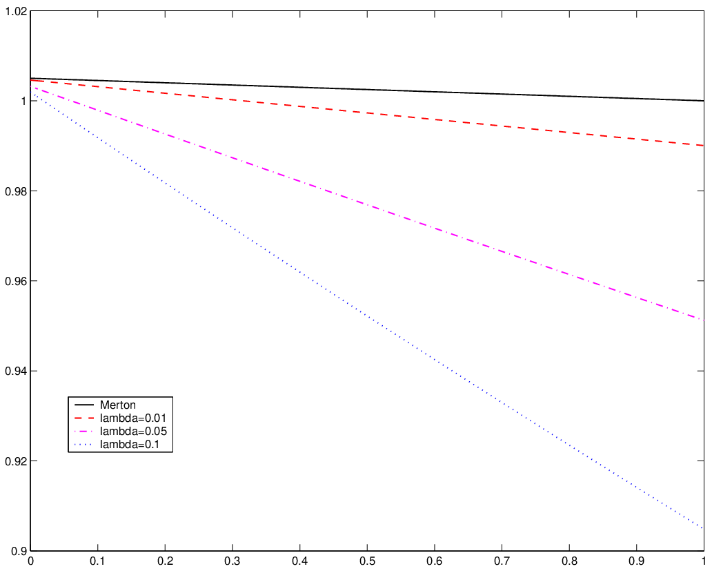
The following numerical results are based on the model parameters described below. We suppose that the survival probability follows the exponential distribution with constant default intensity, i.e. G⁡(t)=e−λ​tG(t)=e^{-\lambda t} where λ>0\lambda>0, and thus the density function is α⁡(θ)=λ​e−λ​θ\alpha(\theta)=\lambda e^{-\lambda\theta}. The functions μd​(θ)\mu^{d}(\theta) and σd​(θ)\sigma^{d}(\theta) are supposed to be in the form

μd​(θ)=μ𝔽​θT,\displaystyle\mu^{d}(\theta)\;=\;\mu^{\mathbb{F}}\frac{\theta}{T}, σd​(θ)=σ𝔽​(2−θT),θ∈[0,T],\displaystyle\sigma^{d}(\theta)\;=\;\sigma^{\mathbb{F}}(2-\frac{\theta}{T}),\;\;\;\theta\in[0,T],

which have the following economic interpretation. The ratio between the after and before-default rate of return is smaller than one, and increases linearly with the default time: the after-default rate of return drops to zero, when the default time occurs near the initial date, and converges to the before-default rate of return, when the default time occurs near the finite investment horizon. We have a similar interpreation for the volatility but with symmetric relation: the ratio between the after and before-default volatility is larger than one, decreases linearly with the default time, converging to the double (resp. initial) value of the before-default volatility, when the default time goes to the initial (resp. terminal horizon) time.

To solve numerically the ODE (4.26), we apply the Howard algorithm, which consists in iterating in (4.27) the control value π\pi at each step of the ODE resolution. We initialize the algorithm by choosing the constrained Merton strategy

π^M\displaystyle\hat{\pi}^{M} =\displaystyle= min⁡(μ𝔽(1−p)​|σ𝔽|2,1γ).\displaystyle\min\Big(\frac{\mu^{\mathbb{F}}}{(1-p)|\sigma^{\mathbb{F}}|^{2}},\,\frac{1}{\gamma}\Big).

In the following Table 1, we show the impact of the loss given default γ\gamma on the optimal strategy π^t𝔽\hat{\pi}^{\mathbb{F}}_{t}. The numerical tests show that except in some extreme cases where both the default probability and the loss given default are large, the optimal strategy is quite invariant with respect to time tt in most cases we consider. So we give below the optimal strategy as its expected value on time. We perform numerical results for various degrees of risk aversion 1−p1-p: smaller, close to and larger than one, and with μ𝔽=0.03\mu^{\mathbb{F}}=0.03, σ𝔽=0.1\sigma^{\mathbb{F}}=0.1, TT == 11 and λ=0.01\lambda=0.01.

Table 1: Optimal strategy vs constrained Merton.
p=0.2p=0.2 p→0p\rightarrow 0 p=−0.2p=-0.2
γ\gamma π^𝔽\hat{\pi}^{\mathbb{F}} π^M\hat{\pi}^{\mathrm{M}} π^𝔽\hat{\pi}^{\mathbb{F}} π^M\hat{\pi}^{\mathrm{M}} π^𝔽\hat{\pi}^{\mathbb{F}} π^M\hat{\pi}^{\mathrm{M}}
0.010.01 3.733.73 3.743.74 2.992.99 3.003.00 2.492.49 2.502.50
0.10.1 3.573.57 3.743.74 2.862.86 3.003.00 2.382.38 2.502.50
0.50.5 1.581.58 2.002.00 1.381.38 2.002.00 1.221.22 2.002.00
0.80.8 0.910.91 1.251.25 0.800.80 1.251.25 0.700.70 1.251.25

First, observe that, when we take into account the counterparty risk, the proportion invested in the stock is always smaller than the Merton strategy without conterparty risk. Secondly, the strategy is decreasing with respect to γ\gamma, which means that one should reduce the stock investment when the loss given default increases.

Table 2: Optimal strategy with various λ\lambda and γ\gamma.
p=0.2p=0.2 p→0p\rightarrow 0 p=−0.2p=-0.2
γ=0.1\gamma=0.1 γ=0.5\gamma=0.5 γ=0.1\gamma=0.1 γ=0.5\gamma=0.5 γ=0.1\gamma=0.1 γ=0.5\gamma=0.5
π^M\hat{\pi}^{\mathrm{M}} 3.753.75 2.002.00 3.003.00 2.002.00 2.502.50 2.002.00
λ=0.01\lambda=0.01 PD=0.01=0.01 3.573.57 1.581.58 2.862.86 1.381.38 2.382.38 1.221.22
λ=0.05\lambda=0.05 PD=0.05=0.05 2.932.93 0.260.26 2.352.35 0.210.21 1.961.96 0.180.18
λ=0.1\lambda=0.1 PD=0.10=0.10 2.222.22 −0.90-0.90 1.781.78 −0.70-0.70 1.491.49 −0.58-0.58
λ=0.3\lambda=0.3 PD=0.26=0.26 0.000.00 −3.96-3.96 0.000.00 −3.00-3.00 0.000.00 −2.40-2.40

Next, we examine the role played by the default intensity λ\lambda. In Table 2, the column PD represents the default probability of the counterparty up to TT with the given intensity λ\lambda, i.e. PD == ℙ⁡(τ≤T)=1−e−λ​T\mathbb{P}(\tau\leq T)=1-e^{-\lambda T}. We see that the stock investment decreases rapidly when the default probability increases. Moreover, when both default probability of the counterparty and the loss given default of the stock are large, one should take short position on the stock in the portfolio investment strategy before the default of the counterparty. Then at the default time τ=θ\tau=\theta, the optimal strategy is switched to π^d​(θ)\hat{\pi}^{d}(\theta), which is always positive.

We also compare the value function obtained in our example to that in the classical Merton model, that is, the solution Y⁡(t)Y(t) to the ODE (4.26) and the function YM​(t)Y^{M}(t) deduced with k⁡(t)=0k(t)=0 and G⁡(T)=1G(T)=1. In Figure 2, the curves represent different values of γ\gamma such that π^M\hat{\pi}^{M} == μ𝔽(1−p)​|σ𝔽|2≤1γ\frac{\mu^{\mathbb{F}}}{(1-p)|\sigma^{\mathbb{F}}|^{2}}\leq\frac{1}{\gamma}. The value function Y⁡(t)Y(t) obtained with counterparty risk is always below the Merton one. It is decreasing on time and also decreasing w.r.t. the proportional loss γ\gamma. In addition, for a given default intensity λ\lambda, all curves converge at TT to G⁡(T)=e−λ​TG(T)=e^{-\lambda T}. In Figure 2, the curves represent different values of λ\lambda. The value function Y⁡(t)Y(t) is also decreasing w.r.t. the default intensity λ\lambda. However, the final value of each curve corresponds to different values of GTG_{T}.

Figure 1: Value function – optimal vs Merton: p=0.1p=0.1, λ=0.01\lambda=0.01.
Refer to caption
Figure 2: Value function – optimal vs Merton: p=0.1p=0.1, γ=0.1\gamma=0.1.
Refer to caption

5 Conclusion

This paper studies an optimal investment problem under the presence of counterparty risk for the trading stock. By adopting a conditional density approach for the default time, we derive a suitable decomposition of the initial utility maximization problem into an after-default and a global default one, the solution to the latter depending on the former. This makes the resolution of the optimization problem more explicit, and provides a fine understanding of the optimal trading strategy emphasizing the impact of default time and loss given default. The density approach can be used for studying other optimal portfolio problems, like the pricing by indifference-utility, with counterparty risk. A further topic is the optimal investment problem with two assets (names) exposed both to bilateral counterparty risk, and the conditional density approach should be relevant for such study planned for future research.

References

  • [1] Bielecki T. and M. Rutkowski (2002): Credit risk: Modeling, Valuation and Hedging, Springer Finance.
  • [2] El Karoui N. (1981): Les aspects probabilistes du contrôle stochastique, Lect. Notes in Math. 816, Springer-Verlag.
  • [3] El Karoui, N., M. Jeanblanc, and Y. Jiao (2009): “What happens after a default, the conditional density approach”, Working Paper.
  • [4] Jacod, J. (1987): “Grossissement initial, Hypothèse (H’) et théorème de Girsanov”, in Séminaire de Calcul Stochastique, (1982/1983), vol. 1118, Lecture Notes in Mathematics, Springer.
  • [5] Jarrow, R. and F. Yu (2001): “Counterparty risk and the pricing of defaultable securities”, Journal of Finance, 56(5), 1765–1799,
  • [6] Jeanblanc, M. and Y. Le Cam (2008): “Progressive enlargement of filtration with initial times”, to appear in Stochastic Proc. and their Applic.
  • [7] Kramkov D. and W. Schachermayer (1999): “The asymptotic elasticity of utility functions and optimal investment in incomplete markets”, Annals of Applied Probability, 9, 904-950.
  • [8] Lim, T. and M.C. Quenez (2008): “Utility maximization in incomplete markets with default”, Preprint PMA, Universities Paris 6-Paris7.
  • [9] Mansuy, R. and M. Yor (2005): Random times and enlargements of filtrations in a Brownian setting, Springer.
  • [10] Wagner D. H. (1980): “Survey of measurable selection theorems: an update”, Lect. Notes in Math. 794, Springer-Verlag.