L.Huijse@uva.nl
Supersymmetry, lattice fermions, independence complexes and cohomology theory
Abstract
We analyze the quantum ground state structure of a specific model of itinerant, strongly interacting lattice fermions. The interactions are tuned to make the model supersymmetric. Due to this, quantum ground states are in one-to-one correspondence with cohomology classes of the so-called independence complex of the lattice. Our main result is a complete description of the cohomology, and thereby of the quantum ground states, for a two-dimensional square lattice with periodic boundary conditions. Our work builds on results by J. Jonsson, who determined the Euler characteristic (Witten index) via a correspondence with rhombus tilings of the plane. We prove a theorem, first conjectured by P. Fendley, which relates dimensions of the cohomology at grade to the number of rhombus tilings with rhombi.
1 Introduction
The motivation for the work presented in this paper is multi-faceted. On the Physics side, the motivation stems from the need to understand the electronic properties of materials where electrons are free to move but subject to strong (repulsive) interactions. Even at the level of relatively simple model Hamiltonians, the behavior of such systems is notoriously difficult to analyze. The model studied in this paper has been chosen such that it enjoys a property called supersymmetry [1]. The benefit of this has turned out to be twofold. First, the supersymmetry leads to a considerable degree of analytic control, allowing the rigorous derivation of quite a few results, in particular on quantum ground states. Second, the sypersymmetric model turns out to have remarkable properties, both in dimension , where the model is quantum critical and described by a superconformal field theory [1, 2, 3], and in dimension , where the model displays extensive ground state entropy [4, 5, 6] and where indications of quantum critical behavior were found [7].
On the Mathematics side the study of supersymmetric lattice models has led to interesting results on the cohomology of independence complexes of lattices and graphs, 2D grids in particular [8, 9, 10, 11, 12, 13, 14]. The two sides are connected by the observation that quantum ground states of the supersymmetric lattice model are in 1-to-1 correspondence with the elements of the cohomology of an associated independence complex.
The supersymmetric model on a 2D square lattice has turned out to be particularly interesting. Numerical results for the Witten index (Euler characteristic) in torus geometry led to remarkable conjectures for the dependence of this quantity on the two periods of the torus [15]. These conjectures were then proven by J. Jonsson [8], using a connection with specific rhombus tilings of the plane. In the present paper we complete the analysis by providing a direct characterization of the elements of the cohomology and thereby of the quantum ground states for the square lattice wrapped around a torus. We prove a theorem, first conjectured by P. Fendley, which relates dimensions of the cohomology at grade to the number of rhombus tilings with rhombi. Since the number of rhombus tilings grows exponentially with the linear dimensions of the system, our result implies that the quantum model has a sub-extensive ground state entropy.
The presentation in this paper is organized as follows. In section 2, we introduce the model and briefly summarize the main results presented in the literature so far. The focus in this section will be on the physics of the model. We then turn to the mathematics side in section 3. We relate the Hilbert space of the supersymmetric lattice model to an independence complex and show that the quantum ground states of the model are in 1-to-1 correspondence with the elements of the cohomology of this complex. At the end of this section, we resume the ’tic-tac-toe’ lemma of [16], which plays a central role in the rest of the paper. In section 4, we state the main result of this paper; a theorem that relates the dimensions of the cohomology at grade to the number of rhombus tilings with rhombi. We briefly discuss how this theorem relates to Jonsson’s work [8, 9] and what the implications for the physics of the model are. The remainder of the paper (section 5) is dedicated to the proof of this theorem. Unfortunately, the proof is quite involved and consists of several steps. A detailed outline of these steps can be found at the start of section 5.
2 Physics connection: supersymmetry and lattice fermions
In this section we will introduce the model and briefly state the main results obtained for this model with a focus on the physics interpretation.
2.1 Supersymmetry
An supersymmetric quantum mechanical theory is constructed from a basic algebra, defined by two nilpotent supercharges and (complex conjugation is implied) [17],
and the Hamiltonian given by
It satisfies
The eigenvalues and eigenvectors of the Hamiltonian give the energy spectrum and the corresponding quantum states. The definition of the Hamiltonian has some immediate consequences for the energy spectrum. First of all, it is positive definite:
for all choices of the quantum state . Second of all, the fact that both and commute with the Hamiltonian, gives rise to a twofold degeneracy in the energy spectrum. In other words, all eigenstates of the Hamiltonian with an energy form doublet representations of the supersymmetry algebra. A doublet consists of two states, and , such that . The states and are said to be superpartners. Finally, all states with zero energy must be singlets: and conversely, all singlets must be zero energy states [17]. In addition to supersymmetry our models will also have a particle-number symmetry generated by the operator with
| (1) |
Consequently, commutes with the Hamiltonian. Furthermore, this tells us that superpartners differ in their fermion number by one (let , then ).
An important issue is whether or not supersymmetric ground states at zero energy occur, that is, whether there are singlet representations of the algebra. For this one considers the Witten index
| (2) |
where the trace is over the entire Hilbert space. Remember that all excited states come in doublets with the same energy and differing in their fermion-number by one. This means that in the trace all contributions of excited states will cancel pairwise, and that the only states contributing are the zero energy ground states. We can thus evaluate in the limit of , where all states contribute . It also follows that is a lower bound to the number of zero energy ground states.
2.2 Lattice fermions
We now make the model more concrete by defining the supercharges in terms of lattice particles. The particles we will consider are spin-less electrons, also called spin-less fermions. Their key property is that the wavefunction is antisymmetric under the exchange of two fermions. It follows that the operator that creates a fermion on site in the lattice and the operator that annihilates a fermion on site in the lattice, satisfy the following anti-commutation relations:
The particle-number operator for fermions is defined as , where the sum is over all lattice sites. This operator counts the total number of particles in a state. A simple choice for the supercharges would be and . It is readily verified that both obey the nilpotency condition and that the commutation relations with (1) are satisfied. However, this choice leads to a trivial Hamiltonian: , where is the total number of sites of the lattice. To obtain a non-trivial Hamiltonian, we dress the fermion with a projection operator: , which requires all sites adjacent to site to be empty. We can now formulate the supercharges in terms of these hard-core fermions: and . Again the nilpotency condition and the commutation relations (1) are satisfied, but now the Hamiltonian of these hard-core fermions reads
The first term is a nearest neighbor hopping term, that is, the fermions can hop from site to site as long as and are connected by an edge and provided that the neighboring sites are empty. The second term contains a next-nearest neighbor repulsion, a chemical potential and a constant. The details of the latter terms will depend on the lattice we choose.
2.3 Results and physics interpretation
This lattice Hamiltonian constitutes a particular instance of an itinerant-fermion system, where all the interactions are fine-tuned by the supersymmetry. Over the last few decades, numerous studies of itinerant-fermion systems in two spatial dimensions have been presented, however, exact solutions are few and far between. The model presented here does allow for exact results and turns out to exhibit quite remarkable features. First of all, the supersymmetric model on the chain can be solved exactly through a Bethe ansatz [1]. In the continuum limit one can derive the thermodynamic Bethe ansatz equations. The model has the same thermodynamic equations as the XXZ chain at , so the two models coincide (the mapping can be found in [2]). The continuum limit is described by the simplest field theory with superconformal symmetry with central charge , which implies that the model is quantum critical. For a periodic chain with length the model has a twofold degenerate zero-energy ground state with fermions.
This ground state degeneracy turns out to be a generic feature of the model. In fact, in two spatial dimensions the ground state entropy typically grows exponentially with the system size. This characteristic of having an extensive ground state entropy goes under the name of superfrustration [4]. Numerical studies of the Witten index have shown that even this lower bound is typically extensive [5]. Exact results for the number of ground states were obtained for various lattices [4]. For example, for the martini lattice, which is formed by replacing every other site on a hexagonal lattice with a triangle, the number of zero-energy ground states was found to equal the number of dimer coverings of the hexagonal lattice. For large systems () this gives
A heuristic way of understanding the superfrustration is from the “3-rule”: to minimize the energy, fermions prefer to be mostly 3 sites apart (with details depending on the lattice). For generic two dimensional lattices the 3-rule can be satisfied in an exponential number of ways.
For certain two dimensional lattices it was proven that zero-energy ground states exist at various fillings. The filling is defined as the number of particles per lattice site. For the square, triangular and hexagonal lattice there exist zero-energy ground states for all rational fillings within the range , and , respectively [9].
The square lattice turns out to be a special case. Here the Witten index is subextensive and for periodic boundary conditions in two directions (i.e. the square lattice wrapped around the torus) it grows exponentially with the linear dimensions of the system [15, 8]. In this paper we prove that the total number of ground states also grows exponentially with the linear dimensions of the system. In fact, this proof establishes a direct relation between ground states and tilings of the plane with two types of rhombi (see section 4 for details), which were first introduced by Jonsson. In [7] we presented numerical studies of various ladder realizations of the square lattice with doubly periodic boundary conditions. These studies, together with the correspondence between ground states and tilings, strongly indicate the existence of critical edge modes in these systems. It is compelling to infer that, if a subextensive systems accommodates edge criticality, a truly extensive system, like the triangular lattice, will allow for bulk criticality. On another speculative note, the ground state-tiling correspondence for the square lattice on the torus suggests the possible existence of topological order in some of the many ground states.
3 Math connection: independence complex and cohomology theory
In this section we will establish the relation between particle configurations of hard-core fermions and independent sets, on the one hand, and between zero energy ground states and cohomology elements on the other. At the end of this section we state the ’tic-tac-toe’ lemma for double complexes, which plays a central role in the proof of the main result of this paper.
3.1 Independence complex
An independent set on a graph is a subset of the vertex set of the graph with the property that no two vertices are adjacent. Since hard-core fermions cannot occupy adjacent sites, it is clear that each allowed configuration of hard-core fermions forms an independent set. In the following we will use the term lattice (i.e. a grid) instead of the more general term graph, since in the physics context it is most natural to study fermions on a lattice. However, the correspondences we establish in this section hold for graphs in general. The family of independent sets of a lattice forms the independence complex of the lattice. We can define the partition sum in the asymptotic (thermodynamic) limit for the independence complex as
| (3) |
where is called the activity. Until recently there were essentially no exact results for independence complexes on two dimensional lattices, with one important exception. Baxter [18] gave an analytic expression for the partition sum of the independence complex on the triangular lattice with positive activity in the thermodynamic limit. This is also referred to as the exact solution for hard hexagons (hard-core fermions on the triangular lattice can, in this context, be viewed as hexagons that share, at most, a side or a corner).
Now observe that the coefficient of in (3) is the number of sets in with size or, in other words, the number of configurations with hard-core fermions. Consequently, gives the dimension of the full Hilbert space ; the space spanned by all possible hard-core fermion configurations. What is even more interesting, however, is that coincides with the Witten index (2)
Recently, Jonsson expressed precisely this quantity () for hard squares on a torus, i.e. with doubly periodic boundary conditions, in terms of rhombus tilings on the torus [8] (see section 4 for details). This quantity coincides with the Witten index for hard-core fermions on the square lattice. For the square lattice the condition that two particles cannot occupy two adjacent sites readily translates to the hard square condition if we define the squares to be tilted by and to have a particle at their center. It follows that the squares cannot overlap, however they can have a corner or a side in common.
3.2 Cohomology and homology theory
It should be clear from the previous that the Hilbert space is a graded vector space, where the grading is defined by the particle-number operator . That is, the Hilbert space can be written as , where is a subspace spanned by all the possible configurations with particles. From the definitions of and and their commutation relations (1) it is clear that is a map from to . Since squares to zero, we can define its cohomology. On the other hand, is a map from to and also nilpotent, so we can define the homology of .
It turns out that the zero energy ground states of the model are in one-to-one correspondence with the non-trivial classes of the cohomology of and the homology of . Remember that all states with zero energy must be singlets: and conversely, all singlets must be zero energy states. Clearly, all singlets, and thus all (zero energy) ground states, are in the kernel of : and not in the image of , because if we could write , then , would be a doublet. Equivalently, we can say that a ground state with fermions is a cycle but not a boundary in . This is precisely the definition of an element of the -th cohomology of , within . Two states and are said to be in the same cohomology-class if for some state . Since a ground state is annihilated by both and , different (i.e. linearly independent) ground states must be in different cohomology-classes of 11 1 Let and be two linearly independent ground states. It follows that . If we now write , we find that and thus . From this we find and thus . With this we obtain , which contradicts our assumption that and are linearly independent, so we conclude that and must be in different cohomology classes.. Finally, the number of independent ground states is precisely the dimension of the cohomology of and the fermion-number of a ground state is the same as the grade of the corresponding cohomology-class. Thus the ground states of a supersymmetric theory are in one-to-one correspondence with the cohomology of . With the same line of reasoning we may also conclude that the ground states are in one-to-one correspondence with the homology of . Finally, the Euler characteristic, defined in cohomology theory as
is precisely the Witten index.
3.3 The ’tic-tac-toe’ lemma
Central to the proof presented in this paper is the ’tic-tac-toe’ lemma of [16]. Let us decompose the lattice into two sublattices and and we write , where and act on and respectively. We can then consider the double complex , where () is the size of the vertex set on (). Equivalently, if we define as the number of particles on , we have and . Finally, we have and . The ’tic-tac-toe’ lemma now tells us that the cohomology of , , is the same as the cohomology of acting on the cohomology of , i.e. , provided that has entries only in one row. That is, is non-vanishing only for one value of (or ).
4 Statement of main result
The main result of this paper can be formulated both in the physics and mathematics context. We prove the result in the mathematics context, namely we find the dimensions of the cohomology for the independence complex on the square lattice wrapped around a torus. In the physics context this translates to the statement that we found the total number of ground states for the supersymmetric model on the square lattice wrapped around a torus. As we mentioned at the end of section 2, the solution is found by relating ground states, or equivalently elements of the cohomology, to tilings of the plane with two types of rhombi. As was mentioned before, this relation is inspired by the work of Jonsson [8, 9]. He first introduced the rhombi when he related the partition sum of hard squares with activity to these rhombus tilings. This is precisely the Witten index for our model on the square lattice, and also the Euler characteristic of . The Witten index is a lower bound to the number of ground states. The result we obtain in this paper gives us, not just this bound, but the total number of ground states with their respective fermion-number in terms of rhombus tilings. A rhombus tiling is obtained by tiling the plane with the rhombi depicted in figure 1, such that the entire plane is tiled and the rhombi do not overlap (they can have only a corner or a side in common). We call the tiles with area 4 diamonds and the ones with area 5 squares.

We can now state the main result of this paper.
Theorem 1.
For the square lattice with periodicities , with a positive integer and , we find for the cohomology
| (43) |
where is the number of zero energy ground states with fermions, is the number of rhombus tilings with tiles, and
with the nearest integer to . Finally, , and
As an immediate consequence of this theorem, we obtain for the Euler characteristic (= Witten index = )
which is precisely the result obtained by Jonsson for the hard squares at activity [8].
Another direct consequence follows from the area of the tiles. The diamonds have area 4, and thus a tiling with solely diamonds will contain tiles. This corresponds to an element in the -th cohomology and a ground state with particles. Conversely, a tiling consisting of squares only corresponds to an element in the -th cohomology and a ground state with particles. Continuing this argument for general tilings with the diamonds and squares, we find on the infinite plane that for all rational numbers the cohomology at grade is non vanishing, or, equivalently, there exists a zero energy ground state with particles. This result was obtained independently by Jonsson [9] for the homology of . In fact, he found that for each tiling there is a so-called cross-cycle, which is a representative of the homology of . However, he could not prove that these cross-cycles are independent, i.e. in different homology classes, nor that they constitute a basis. A comparison with our result, theorem 1, suggests that the cross-cycles are indeed independent and span the full homology with the exception of elements at the -th grade.
Finally, the theorem provides insight in the growth behavior of the number of ground states, since this is now directly related to the growth behavior of the number of tilings. In [10] various results on the number of tilings on the doubly periodic square lattice are reported. Here we mention two of these results for the case that and .
- 1
For and such that , there are no rhombus tilings that satisfy the periodicities given by and .
- 2
For and , with and positive integers and large, the total number of rhombus tilings grows as
In the first case it follows that the number of ground states with particles is given by , which is non-zero only for given that . In the second case the number of ground states will show the same growth behavior as the number of tilings. This number turns out to be dominated entirely by the number of tilings with tiles. Furthermore, it is noteworthy that the number of tilings grows exponentially with the linear dimensions, instead of the area, of the system. It follows that, eventhough the system is highly frustrated, this leads only to a sub-extensive ground state entropy. This is in contrast with results obtained for the triangular, hexagonal and martini lattices, for which the ground state entropy was found to be extensive [4, 5].
5 Proof of main result
In this section we present the proof of theorem 1. Unfortunately, the proof is quite involved and consists of several intermediate steps. Here we will give a brief outline of these steps. In section 3.3 we resumed the ’tic-tac-toe’ lemma which plays a crucial role in the proof. The lemma relates to and when is written as . This is achieved by writing the lattice as and letting act solely on . The crucial step is to choose the right sublattices. It turns out that for the square lattice one should pick a set of disconnected points for and a set of (disconnected) chains for (for the details see definition 2).
First, in section 5.1, we will discuss the cohomology results for a single chain with various boundary conditions. These results are crucial in the first step of the ’tic-tac-toe’ lemma, i.e. computing the cohomology of , since acts on a set of chains.
Second, in section 5.2, we consider the square lattice on the plane and on the cylinder, to illustrate the power of the ’tic-tac-toe’ lemma for a relatively simple case. We choose the boundary conditions in such a way that is non-vanishing only for one value of and . Consequently, and are trivially obtained from .
Finally, we wrap the square lattice around the torus. We then apply the same strategy as in section 5.2, and is easily obtained. Unfortunately, however, it has entries in several rows and columns of the double complex and computing is highly non trivial.
As a first step (section 5.3.1), we compute for a thin torus, such that the sublattice consists of one chain only. For this case, we then show that , even though has entries in multiple rows. The final step for this simple case is to relate the elements of to periodic sequences of tiles and identify the elements that give rise to the small number in (43).
In the last step (section 5.3.2), we finally present the proof of theorem 1. Here the sublattice consists of an arbitrary number of chains. We proceed as in section 5.3.1 to obtain and each step will be similar, but slightly more involved. Again we find that does not have entries only in one row. In contrast to the thin torus case, however, we find that here is contained in but not equal to . Using the ’tic-tac-toe’ procedure, we reduce to obtain . What we find is that all the elements of can be obtained by concatenating so-called building blocks and in the final step we map each building block to a sequence of tiles. It follows from this mapping, that the elements of map to all possible tilings, again with a small discrepancy , which is computed in the very last step.
5.1 The cohomology of on the chain
In the following sections we will often use the cohomology results for the supersymmetric model on the chain. These results can be found in [2, 1], but will be restated here for completeness.
Definition 1.
An open chain of length is the graph with vertices and edges . A periodic chain of length is a cycle defined by the graph where .
In the following ( can also be zero as long as the number of sites is positive).
Theorem 2.
The cohomology of on the periodic chain with sites has:
- •
2 non-trivial cohomology classes with fermions if ,
- •
1 non-trivial cohomology class with fermions if .
The cohomology of on the open chain with sites has:
- •
1 non-trivial cohomology class with fermions if or ,
- •
0 non-trivial cohomology classes if .
Proof.
We prove this result for the periodic chain with sites. We take to be every third site and the remaining sites . Remember that is the number of fermions on sublattice . Consider a single site on . If both of the adjacent sites are empty, is trivial: acting on the empty site does not vanish, while the filled site is acting on the empty site. So the empty site does not belong to the kernel of , whereas the filled site belongs to the image of . This leads to a vanishing , unless every site on is forced to be empty by being adjacent to an occupied site. There are only two such configurations:
| (50) |
where the square represents an empty site on . Both states and belong to : they are closed because , and not exact because there are no elements of with fermions, where . By the ’tic-tac-toe’ lemma, there must be precisely two different cohomology classes in , and therefore exactly two ground states with fermions. ∎
The proofs for the other cases are completely analogous. In the main proof we will need the representatives of the non-trivial cohomology classes of on the open chain. We will use the following notation: to denote a configuration with fermions on sites , , , etc. we write .
Lemma 1.
A representative of the non-trivial cohomology classes of on the open chain with or sites is
| (51) |
where on the dots the numbers always increase by three.
Proof.
From theorem 2 we know that the representative has fermions. In the case that it follows that is the only configuration with fermions that belongs to the kernel of . Since the dimension of is one, must be a representative of the non-trivial cohomology class.
When there are two configurations that belong to the kernel of : and , however the dimension of is again just one. It follows that a linear combination of these two configurations will be in the image of . In general, two states and are in the same cohomology class if one can write for some state . In that case both and are good representatives of the cohomology class. Since itself is not in the image of it is thus a good representative. ∎
5.2 The cohomology of on the square lattice. Part I: Tilted rectangles and cylinders
Let us define with as the subset of given by the points such that
| (52) |
This defines a tilted rectangular part of the square lattice. We can also define with as the subset of given by the points such that
| (53) |
Whereas contains the point , it is excluded in . The lattice can be mapped to a lattice of the former type except when and are both odd. Finally, for even the cylindrical version can be obtained from by identifying the vertices and .
For the lattices , and the full cohomology problem has been solved using Morse theory [12]. These cases can also be solved using the ‘tic-tac-toe’ lemma. The crucial step is to choose the right sublattices. We take a set of disconnected sites for and a set of (open or periodic) chains for (see fig. 2).
Definition 2.
More formally, for is the set of points that satisfy
| (54) |
with and is the set of points that satisfy
| (55) |
with . The sublattices can be defined similarly for .

To solve we start from the bottom-left chain. If a site on directly above this chain is occupied, we are left with an isolated site on the bottom-left chain (see fig. 3), leading to a vanishing (see section 5.1). It follows that all sites directly above the bottom-left chain must be empty. Continuing this argument for subsequent chains one finds that all sites on must be empty. However, in the case that we have a set of disconnected sites at the top-right that belong to . From the previous argument we obtained that the sites of directly below the top-right sites of have to be empty. This implies that for vanishes. When we find that all elements in have all sites in empty, thus computing is a trivial step. The dimension of is related to the number of ground states, or equivalently, the number of non-trivial cohomology classes of on the chains that constitute . Note that the length of these chains is both for the tilted rectangles as well as for the cylinder. In the first case the chains have open boundary conditions, whereas in the latter the chains are periodic. Now, the number of non-trivial cohomology classes of for all these cases can be found in theorem 2.

It follows that for the tilted rectangles, and , with we have
- i)
no non-trivial cohomology classes for
- ii)
one non-trivial cohomology class for .
For the cylinder, , with and even we have
- i)
one non-trivial cohomology class for
- ii)
non-trivial cohomology classes for , with the nearest integer to .
For the non-trivial cohomology vanishes for both the rectangle and the cylinder.
5.3 The cohomology of on the square lattice. Part II: The torus
We now define the doubly periodic lattices via two linearly independent vectors and
. We wrap the square lattice around the torus by identifying all points with
.
The main result of this paper is that we find the full cohomology of on the square lattice with doubly
periodic boundary conditions defined by and such that . In
particular, we obtain a direct relation between elements of and tiling configurations. This relation
allows us to prove theorem 1, that was first conjectured by P. Fendley and is strongly
inspired by the work of Jonsson [8, 9]. It is restated here for convenience.
For the square lattice with periodicities , with a positive integer and , we find for the cohomology
where is the number of zero energy ground states with fermions, is the number of rhombus tilings with tiles, and
with the nearest integer to . Finally, , and
Computing the cohomology for these tori is far from trivial. First of all, computing does not imply that all sites on are empty, instead there are many allowed configurations on . Secondly, because of this, computing becomes much more involved. Finally, we will see that, generally, will be contained in , but not equal to .
We will divide the proof into two parts. We start by proving the theorem for a specific torus, defined by and . This proof will already contain many steps that we use in the proof for the more general case, however, it will be deprived of certain complications. For instance, here we will find . As we said, this is not true in general, and in the second part of the proof a substantial part will be concerned with obtaining once we have found .
5.3.1 A special case: consisting of 1 chain
In this section we consider the case where and . It follows that consists of exactly one periodic chain (see fig. 4).

The proof of theorem 1 for this case will consist of 4 steps:
- 1.
We compute .
- 2.
We compute and show that its elements can be constructed from a finite number of building blocks, called motifs. A motif is characterized by a certain configuration on a finite number of subsequent sites.
- 3.
We show that .
- 4.
We relate the elements of to tiling configurations by relating each motif to a small series of tiles.
Step 1
First we compute and we find the following:
Lemma 2.
The cohomology of consists of all possible configurations on except for configurations with a multiple of three sites empty between two occupied sites.
Proof.
The proof is relatively simple. First note that when a site on is occupied, it blocks four subsequent sites on the chain (see fig. 4). By occupying sites on the periodic chain is cut into smaller pieces of chain with open boundary conditions. Consequently, vanishes when at least one of these smaller pieces has length . This happens when the number of empty sites between two occupied sites on is a multiple of three. We conclude that all configurations on are allowed except for configurations with a multiple of three sites empty between two occupied sites. ∎
Step 2
This step in the proof is the most involved. In the next section, where we prove theorem 1 in all generality, we will often refer back to the results obtained in this step. In this step we compute , where was obtained in the previous step. Let us define and as the number of fermions on and respectively. Furthermore we shall adopt the following notation: an empty site on is denoted by 0 and an occupied site is denoted by 1. A configuration on can then be written as a series of 1’s and 0’s. In the following we shall consider all possible types of configurations on that belong to and we shall investigate if they also belong to .
If we consider a configuration on , we note that there have to be at least two adjacent, empty sites to allow for . This is because two adjacent empty sites leave an open chain of two sites unblocked on and this has an element in with . A typical configuration will thus consist of alternating segments, where a segment is a sequence of sites. The segments are characterized by the number of fermions on the part of the chain corresponding to the segment, this is either zero or greater than zero. In a segment with all sites are empty and it contains at least two sites. On the other hand, a segment with can have empty sites on , but the empty sites cannot be adjacent. Finally, a segment with will always start and end with an occupied site. We will call this pair of occupied sites a pair of bounding sites. Note that a segment with can consist of a single occupied site, in that case the bounding sites fall on top of each other and the pair of bounding sites is just this one site.
Example 1.
Consider the configuration ””, there are two segments with , formed by the first nine sites and the fourteenth site respectively. There are also two segments with constituted by the rest of the sites. Finally, the first and the ninth site form a pair of bounding sites.
First, we consider the segments with .
Lemma 3.
acting on a segment with gives zero within .
Proof.
Suppose this segment between a pair of bounding sites consists of empty sites. The corresponding chain then has length . Since , we find or . For these chain lengths the elements of the cohomology of have and fermions respectively. We now distinguish two cases: a) acts on a site at the boundary of the segment, b) acts on a site away from the boundary.
a) In this case the length of the chain in the new configuration is . Thus or . On the new chain there are still or fermions respectively. However, theorem 2 states that the cohomology for chain length () vanishes at all fermion numbers except (). Thus the new configuration does not belong to and it follows that this action of within gives zero.
b) In this case the action of cuts the chain into two smaller chains of lengths and . Their total length is , since the occupied site now blocks 4 sites on the chain. For we have and or and , where in both cases . For the latter case vanishes at all grades. In the first case is non-vanishing only for . However, the number of fermions on the chains in the new configuration is and thus is does not belong to . Similarly, one finds that for , the new configuration does not belong to . Again we obtain that this action of within gives zero.
Finally, if the segment with extends over the entire system, we are always in the case considered under b). However, the original chain length can now also be with fermions on it. Under the action of we obtain a new chain of length , which has a non-vanishing cohomology if and only if . So also in this case we find that the action of gives zero within .
∎
Second, we consider the segments with .
Lemma 4.
vanishes when the number of sites between any pair of bounding sites in a segment with , is and it contains one element otherwise.
Example 2.
Consider a configuration with one empty site between a pair of bounding sites: ””, this is not an element of , since on this configuration gives ””, which is also in . Now consider two sites between a pair of bounding sites. Then there are two configuration with one empty site: ”” and ”” and one configuration with all sites occupied ”” (remember that the configuration ”” does not have ). It follows that acting on (”” ””) gives ””, whereas acting on (”” ””) gives zero22 2 Note that the fermionic character of the particles is reflected in the sign here: acting on ”” gives ””, whereas acting on ”” gives ””. In the first case the particle is created on position 2 and has to hop over the particle at position 1, this gives a minus sign, in the second case the new particle is created at position 3 and thus has to hop over two particles, giving rise to no overall sign change. Also note that the states are not properly normalized, but this is not important for the argument.. Consequently, we find that consists of one element: the sum of the configurations with .
Proof.
We can solve for an arbitrary number of sites between a pair of bounding sites, by realizing that this problem can be mapped to the normal chain. For the normal chain no two fermions can be adjacent, whereas here no two empty sites can be adjacent. So we can map empty sites to fermions on the chain and occupied sites to empty sites in the normal chain. Finally, is mapped to on the normal chain. For the chain (which has the same dimension as ) vanishes when the length of the chain is and it contains one element otherwise. So here we have that vanishes when the number of sites between two occupied sites is and it contains one element otherwise.
∎
For a segment with , let us denote the representative of by the pair of bounding sites with dots in between, for example we denote (”” ””) by ””. Even though, this is now a sum of configurations, we will still refer to this simply as a configuration. It follows that, for a segment with , two types of configurations are allowed. The two types can be distinguished by containing dots or dots. Examples of the first type are: ””, ””, ””, etc. Note that the configuration with , and thus with -1 dots between the pair of bounding sites, is ””. Examples of the second type are: ””, ””, ””, etc.
Combining lemma’s 3 and 4, we find
that is spanned by all
configurations that can be formed by concatenating the following motifs:
””
””
””
””
””
where means dots and, as before, ”” with means ””.
Finally one can also have all zeroes for any length and all dots for any length. Note that if the number of sites is a multiple of three, that both the configuration with all zeroes and the one with all dots account for two linearly independent elements of . This is because the cohomology of acting the periodic chain with length a multiple of three has dimension two (see theorem 2).
Example 3.
As an example, suppose we have as always and . This implies that consists of 10 sites and with the defined motifs it follows that the following 12 elements belong to : ””, ””, ””, ””, ””, ””, ””, ””, ””, ””, ”” and ””. Note that the first nine motifs have periodicity 10 and thus account for ten elements of each, whereas the motif ”” has periodicity 5 and the last two motifs have periodicity 1. For each element one can easily compute the number of fermions and it follows that the first nine motifs have 7 fermions, the motif ”” has 6 fermions and the last two motifs have again 7 fermions. So in total we have 92 elements in with 7 fermions and 5 elements with 6 fermions.
Step 3
In the previous step we have obtained for . In this step we show that in this case this is equal to the cohomology of . We do this via the ’tic-tac-toe’ procedure [16]. That is, we act on a configuration, say , with . The part will automatically give zero, but the part not necessarily, since we no longer restrict ourselves to the subspace . If it does give zero, we know that the configuration belongs to the kernel of . The configuration will thus belong to unless it also belongs to the image of . In that case, another configuration will map to this configuration at the end of the ’tic-tac-toe’ procedure. So we continue with the configurations, , that do not belong to the kernel of . Since the image of does not belong to and it does belong to the kernel of , it must also belong to the image of . So we can write , for some configuration . Now let us define a new state . It then follows that . If this is zero, we have found that the state belongs to the kernel of . If it is non-zero we proceed as before: we try to find a configuration , such that and define a new state , etc. This procedure ends, either when we have found a state such that , or when with an element of . In the latter case, we say maps to at the end of the ’tic-tac-toe’ procedure and we conclude that neither nor belong to .
For the case we consider in this section, we will show that for each element , there is an element that belongs to the kernel of . So for each element in we can find a corresponding element in , thus we obtain . In the next section, however, we will see that this is not true for general boundary conditions. We will then find that after several steps in the ’tic-tac-toe’ procedure we map certain configurations in to other configurations in . It follows that the first do not belong to the kernel of and the latter belong to the image of . In that case is strictly smaller than .
Lemma 5.
for and .
Proof.
For the segments with , we found that vanishes if we choose the states represented by the dots such that they are ground states of the normal chain with empty and occupied sites exchanged (see lemma 4). For the segments with , we know from lemma 3 that the new configuration always belongs to the image of . That is, , for some configuration if acts on a segment with . So we can define a new configuration , such that . Now either acts on a different segment with , in which case the new configuration again belongs to the image of , or it acts on the same segment. In the latter case the new configuration is cancelled by the same configuration in which the two sites are occupied in the reverse order due to the fermionic character of the particles. It thus follows that the ’tic-tac-toe’ procedure always gives zero after as many steps as there are segments with . ∎
Step 4
In this final step we will show that the dimension of (and the fermion number of each state) can be computed by counting all tiling configurations (and the number of tiles per configuration) with the four types of tiles depicted in figure 1. For the boundary conditions we consider here, the tilings reduce to a single layer sequence of only two types of tiles. Namely the two tiles that respect the boundary condition . These tiles have two edges parallel to and then the diamond has the other two edges parallel to whereas the square has the other edges parallel to (see fig. 5). Given the sublattices and there are three types of vertices: the ones that belong to , the lower left sites of the -chain and the upper right sites of the chain. It follows that the diamond has one of three types of edges along the direction and a matching type of edge along the direction, the square can have one of three different types of edges along the direction and a matching type of edge along the direction. We conclude that we have 6 types of tiles, depicted in figure 5.


To establish theorem 1 we map each of the motifs obtained in step 2 to a unique sequence of tiles. The mapping for the four basis motifs, ””, ””, ”” and ””, is shown in figure 6. Remember that each motif is modulo the addition of 3 zeroes and modulo the insertion of 3 dots. In terms of tilings, we find that each basis motif can be followed by an arbitrary repetition of the tiling corresponding to the 3 zeroes (see fig. 7). On the other hand, insertions of multiples of 3 dots correspond to inserting multiples of the tiling shown in figure 7 at the dotted line along the direction in the basis motifs. Some examples are shown in figure 7. Note that here we cannot easily write the motif of dots directly in the tiles (see fig. 7), however, the mapping is still unambiguous.


Let us determine the number of fermions per motif. First of all, in a segment with , the number of fermions is determined by the length of the corresponding chain. It is easily verified, that for a segment with empty sites the corresponding chain has length . Moreover, from theorem 2, we know that an element in the cohomology of on a chain with length contains fermions, where is the nearest integer to . Similarly, we find that a segment with dots contains fermions. Thus a segment with , consisting of dots and a the pair of bounding sites, contains fermions. From these formulae we find for the four basis motifs ””, ””, ”” and ””, that they contain 2, 3, 3 and 4 fermions respectively. Furthermore, an insertion of 3 zeroes, corresponds to increasing by 3, and thus increasing the number of fermions, , by 2. Equivalently, inserting 3 dots corresponds increasing by 3, and thus again increasing the number of fermions, , by 2. If we compare this to the number of tiles in the tilings that correspond to these motifs, we find that they exactly agree. Furthermore, the number of sites in a motif is given by three times the number of sites in a motif, since there are 2 sites for every site. On the other hand, for the tiles we find that the area of the diamond is 4 and the area of the square is 5. It is now easily verified that the number of fermions per site for the motifs is the same as the number of tiles per area for the corresponding tiling. Thus we find that, not only is the number of elements in the cohomology of directly related to the number of tilings with the two tiles of figure 5, but also the number of fermions for each element corresponds to the number of tiles in the corresponding tiling.
One can verify that with these sequences of tiles, and the rules for concatenating them, one can obtain every possible tiling. Each tile can be preceded by a certain type of square and diamond and it can be followed by another type of square and diamond. In total this gives four possibilities for the surrounding neighbors. It can be checked that for each tile all four possibilities can be constructed with the given sequences of tiles and the rules for concatenating them.
Finally, the configurations with all zeroes or all dots account for the extra term in (43) in theorem 1 repeated here for convenience:
Remember that
and with and we have , and . It follows that the extra term is for and otherwise.
Let us consider the configuration with all zeroes, which clearly has periodicity 1. If the number of zeroes is a multiple of three, i.e. , the configuration accounts for 2 ground states, otherwise it accounts for 1 ground state. The number of fermions in this configuration is , i.e. the nearest integer to . From the mapping (fig. 7) it is clear that the configuration corresponds to a tiling with periodicity 3 if . If , however, there is no corresponding tiling. Exactly the same holds for the configuration with all dots. It follows that for the tilings overcount the number of ground states by 2 and for the tilings fail to count 2 ground states.
Note that the choice of sublattices and has increased the number of tilings unrelated by a lattice symmetry by a factor of three (see fig. 5). Indeed when computing the number of ground states with the motifs given in step 2 it turns out that one discovers each tiling three times (given that the tiling is not completely uniform, that is all diamonds or all squares).
Example 4.
Let us consider the case of example 3 again. So we have and . One possibility is to cover the lattice with 6 squares. This tiling has a unit cell of size 5 and thus this tiling accounts for 5 ground states. The number of tiles is 6 and thus the ground states will have 6 fermions. We can also cover the lattice with 2 squares and 5 diamonds. The 2 squares can be placed between the diamonds in three independent ways. Each of these three tilings has a unit cell of size 30 and consists of 7 tiles, so they account for 90 ground states with 7 fermions.
We compare this with the 12 configurations found in example 3. The motif ”” has periodicity 5 and accommodates 6 fermions, so this corresponds to the uniform tiling with all squares. The configurations with all zeroes and all dots account for two ground states with 7 fermions and have no corresponding tiling. Finally, there are 9 configurations with periodicity 10 and 7 fermions, which account for 90 ground states. Using the mapping given in figure 6, we find that these configurations can be split into three groups of three, each group corresponding to one of the tilings with 2 squares and 5 diamonds. For example the motifs ””, ”” and ”” correspond to the tiling where the two squares are adjacent. They can be distinguished by considering for example the first of the two squares. In each motif it will be of a different type, where the three types are given in figure 5 (see fig. 8).

5.3.2 The general case: consisting of chains
In the previous section we had . In this section we relax this condition to with with a positive integer. It follows that we get chains with their accompanying sites stacked on top of each other. For this situation we will prove theorem 1. The proof consists of 5 steps:
- 1.
We compute .
- 2.
We compute .
- 3.
We compute starting from via the ’tic-tac-toe’ procedure.
- 4.
We relate the elements of to tiling configurations by relating each motif to a small series of tiles.
- 5.
We compute .
Step 1
As in the previous section we shall start by computing the cohomology of . We will define two types of configurations that do not belong to and then find that consists of all configurations except these two types.
Lemma 6.
A configuration that contains an occupied site on the lattice, such that the sites and and/or the sites and are empty, does not belong to .
Proof.
It is easily verified (see fig. 9) that in this configuration the sublattice contains the isolated site(s) and/or . This site can be either occupied or empty, which leads to a vanishing . ∎

Note that in the previous section this situation never occurred because for each occupied site , the sites and were automatically occupied due to the boundary condition set by . The second type of configuration that does not belong to follows from a generalization of lemma 2. Remember that occupying sites causes the chains to break into smaller open chains. The length of these open chains now depends on the number of empty sites directly below and above the chain. For an example see figure 10.
Lemma 7.
If, for a certain configuration, the sum of the number of empty sites directly below and above an open chain is , the configuration does not belong to .
Proof.
It is easily verified that the open chain corresponding to the empty sites has length . This leads to a vanishing . ∎

A configuration does not belong to if it contains one or more isolated open chains on the sublattice with length . It is easy to see that all such configurations fall into the class of configurations described in lemma 6, or lemma 7, or both. It follows that all configurations that do not fall into either of these classes belong to .
Step 2
As in the previous section, we will now compute .
Definition 3.
Define a row of sites as the set of sites directly above one chain.
Note that the configurations in again contain segments where , the number of fermions on the sublattice, is zero and segments where it is non-zero.
Lemma 8.
Lemma 4 for holds for each row of sites.
That is, in the segments where , the cohomology of vanishes when the number of sites between any pair of bounding sites is and it contains one element otherwise. The proof can be found in the previous section. It follows that, in the segments where , two types of configurations on a row of sites are allowed. Using the notation of the previous section, the two types can be distinguished by containing dots or dots.
Lemma 9.
The configurations in have spatially separated columnar segments where and segments where . The width of a column in a segment where can vary between and sites, whereas the width of a column in a segment where can vary between and sites. In the latter case, two consecutive rows never both have width and the difference in their widths is at most 1 (or -1).
An example is shown in figure 11. From lemma 9 it follows that we only have to consider columns of width varying between 1 and 2 in the segments where separated by columns of width varying between 2 and 4 in the segments where . All other configurations can be obtained from these configurations by inserting multiples of 3 dots in the segments where over the entire height of the columns, and, similarly, by inserting multiples of 3 zeroes in the segments where over the entire height of the columns.

We now turn to the segments where . Remember that in the previous section this step was easy because all sites in the segment where were blocked by fermions on the chain. Here, however, that is not the case. The first thing we note in this case is the following.
Lemma 10.
The sites within a column marking a segment where have to be empty if they are away from the boundaries with adjacent columns marking a segment where .
Proof.
This follows directly from lemma 6. ∎
From this lemma it follows that we only have to consider the sites on the boundary between a segment where and a segment where . In fact, we will argue that we only have to consider the boundary where the segment with is to the right of a segment with (and not the boundary on the other side).
First, however, we introduce a new notation where a configuration is fully characterized by the boundaries between the two types of segments ( and ). From lemma 6 it follows that these boundaries are an arbitrary sequence of steps of and . However, in the new notation we shall tilt the lattice by , such that the rows of sites are horizontal. If we then draw the boundary as a collection of vertical lines between two sites that are to the left and to the right of the boundary, we find that the boundaries have a zigzagged shape. The segments where will be white and the segments where will be grey. For an example see figure 12.

Suppose for a moment that we would have a completely disconnected graph, that is, just a collection of disconnected vertices. Then each site can be both empty and occupied. It is clear that each configuration with a least one empty site does not belong to the kernel of , whereas each configuration with at least one occupied site belongs to the image of . It follows that vanishes at all grades. Here we do not have a disconnected graph, however, it turns out that the division in grey and white regions is similar to disconnecting the graph.
We define a special notation for a site that can be both empty and occupied. If this site is to the right of a grey region we shall denote this site with a dot, whereas when it is to the left of a grey region the site will be shaded. That is, suppose there are two configurations that both belong to and obey lemma 9, such that these two configurations differ by one site only. Then we can summarize these two configurations in one picture by denoting this particular site by a dot if it is to the right of a grey region or by shading the site if it is to the left of a grey region. For an example see figure 13. Moreover, we can summarize configurations in one picture if the picture contains sites with dots or shaded sites. We make a distinction between sites to the left and to the right of the grey region, because we will argue that the configurations with a site with a dot do not belong to . Clearly this is a choice, we could also have chosen to argue that the configurations with a shaded site do not belong to .
Let us consider a boundary that separates a grey segment on the left from a white segment on the right. There are only a few such configurations that may have a site on the boundary with a dot.

Lemma 11.
There are 8 possible configurations with a site with a dot in a boundary that separates a grey segment on the left from a white segment on the right. The configurations are depicted in figure 14.
Proof.
The first restriction follows from lemma 6. That is, both when the site is empty as well as when it is occupied, the configuration should satisfy the lemma. This restriction is depicted in figure 14. Then the second restriction follows from lemma 8, that is, the width of a grey column varies between 1 and 2 modulo 3. It follows that next to the site with the dot there can only be one grey site (modulo 3). Combining this again with lemma 6, we find four possibilities for the left boundary of the grey segment. The four possibilities can be summarized in one picture with the notation defined above, see figure 14, the shaded sites can be both empty and occupied. Finally, it follows from lemma 7 that there are only two possible right most boundaries for the white segment, each modulo columns of width 3, see figure 14. ∎


From lemma 11 it follows that if there is more than one site with a dot in the same boundary, they are sufficiently far away to be independent. That is, each of these sites can be both empty and occupied independent of the configuration of the other dotted sites. Also note that if we select one of the 8 configurations with a dot from figure 14, the rest of the system can take on any configuration independent of the configuration of the dotted site. Note that this resembles a disconnected graph.
We are now ready to solve .
Lemma 12.
All configurations that contain a boundary between a grey segment to the left and a white segment to the right, such that this boundary contains one or more sites with a dot, do not belong to .
Proof.
A site with a dot can be either empty or occupied. Suppose the site is empty and we act with on the configuration. If can act non-trivially only on the site under consideration we are done, since the configuration in which the site with the dot is empty does not belong to the kernel of and the configuration in which it is occupied belongs to the image of . This proves the lemma for this case.
If, however, can act non-trivially also on other sites, there are four scenarios: a) The other site is in the same boundary. b) The other site is in the left boundary of the grey region under consideration. c) The other site is in the right boundary of the white region under consideration. d) The other site is further away from the region under consideration than the first three cases.
For scenario a), we know that the other site is also a site with a dot. It follows that the configuration with both dotted sites empty does not belong to the kernel of . The sum of the configurations with one of the dotted sites empty belongs to the image of . The difference of the configurations with one of the dotted sites empty does not belong to the kernel of , because it maps to the configuration with both dotted sites occupied. Clearly, the latter configuration belongs to the image of . So for this scenario the lemma is proven.
For scenario b) we distinguish two cases. First, the other site and the dotted site can be occupied simultaneously. In this case we can prove the lemma via the same argument as we did for scenario a). Second, the other site and the dotted site cannot be occupied simultaneously. This only happens when the other site is in the same row as the dotted site. In this case the sum of the configurations with one of them occupied is in the image of , but the difference belongs to the kernel of and does not belong to the image of . The latter is thus an element of . However, we have the freedom to decide to keep only the configuration in which the other site is occupied and the dotted site is empty as a representative of this element. At this point it becomes clear why we only consider configurations with a site with a dot, and not configurations with a shaded site.
For scenario c) we can again distinguish two cases. In the first case, the configuration of the other site and the dotted site are independent and the lemma is proven as for scenario a). In the second case, the other site and the dotted site cannot be occupied simultaneously. There are again three configurations under consideration. The configuration with both sites empty does not belong to , the sum of the configurations with one of the two sites occupied belongs to and, finally, the difference again is an element of . And as under b), we choose to represent this element with the configuration where the dotted site is empty and the other site occupied.
Finally, for scenario d) it is clear that the configuration of the other site and the dotted site are always independent and the lemma is proven as for scenario a).
In the four scenarios we considered, there was just one other site on which acts non-trivially. If there are more sites on which acts non-trivially, the lemma clearly holds when these sites can again be empty or occupied independent of the dotted site. However, if they are not all independent, the proof is more lengthy, but analogous to the proofs of the second case in scenarios b) and c).
∎
Lemma 13.
All the configurations that belong to are a sequence of alternating grey and white columns subject to the conditions in lemma 9, such that the left-most boundary of all the white columns does not contain any sites with a dot.
Proof.
This is a direct consequence of lemma 12. ∎
As an example we consider the case where and , that is, we stack four rows of sites separated by four chains. All configurations in can be obtained by concatenating the configurations depicted in figure 15, with eventual insertions of grey and/or white columns of width 3, such that the boundary conditions are satisfied33 3 These configurations are obtained as follows. First consider all possible white segments satisfying the boundary condition in the -direction, then construct all possibilities for the grey segments to the left of these white segments.. That is, each row should in the end have width or, equivalently, the right-most boundary should fit with the left-most boundary. Finally, there is a configuration with all zeroes (one entirely white segment) and a configuration with all dots (one entirely grey segment).

Step 3
In the previous step we have determined . According to the ’tic-tac-toe’ lemma, the cohomology of is equal to or contained in : . In the previous section we found that for , we have . For general , however, this is not the case. That is, within , there are configurations that are not in the kernel of and there are configurations that are in the image of . To find out which configurations do not belong to , we follow the ’tic-tac-toe’ procedure [16] as described in step 3 of section 5.3.1.
In the previous section, we found via the ’tic-tac-toe’ procedure that we could find for each element , that belongs to , but not to , an element that does belong to . In this section, however, we will find that for some elements , the ’tic-tac-toe’ procedure leads to a corresponding element , that also belongs to . We then say that maps to at the end of the ’tic-tac-toe’ procedure and we conclude that neither nor belong to .
We now prove some rules for the ’tic-tac-toe’ procedure specific to the configurations we obtained in the previous step.
Lemma 14.
Let act on an empty site , such that for the preceding sites on that row we have: and are occupied and the intermediate sites are dotted. Then the new configuration with occupied, is also the image of acting on the configuration with occupied and one less fermion in the preceding sites to .
Proof.
For general we can denote the original configuration as ””, the new configuration is then ””. From lemma 4 we know that, if the number of sites between a bounding pair is , vanishes. Consequently, each configuration that is in the kernel of is also in the image of . Now, since the configuration ”” is in the kernel of and the number of sites between the bounding pair is , it must also be in the image of . Thus, there is a configuration with one less fermion between the bounding pair that maps to this configuration under the action of . ∎
Example 5.
For this is easily understood: the original configuration will have ”” on the sites through . Acting on this with gives ””, however, this can also be obtained by acting with on -””.
Lemma 15.
Acting with on a white segment away from the boundary, gives zero.
Proof.
The proof is analogous to the proof of lemma 3. The length of the chains in the white region is or each containing fermions. If acts on a site above this chain and away from the boundary, it will cut the chain into 3 pieces. One of length 1 and two of lengths and , such that . We will now argue that the new configuration with the smaller chains, always belongs to . This implies that we can always continue to the next step in the ’tic-tac-toe’ procedure.
If the chain of length 1 contains a fermion, the new configuration clearly belongs to . If it is empty there are fermions on the other two chains. For their combined length is , so and or and , where in both cases . For the second case the cohomology vanishes for all fermion numbers because of the length . For the first case the cohomology is non-vanishing only if , however, there are fermions. So for both cases the new configuration belongs to (since it belongs to and not to ). For we find and or and , where in both cases . The rest of the argument is the same as before.
From the above it follows that we can always continue with the next step in the ’tic-tac-toe’ procedure. Now suppose that in this next step we act with on the same row as in the first step. Since there are no fermions between these two sites, this configuration will cancel against the configuration where the two sites are occupied in the reverse order. It follows that we only have to consider acting with on each row just once.
It is now easily verified that, since there are as many chains as there are rows, we can always continue the ’tic-tac-toe’ procedure until we get zero. ∎
In this lemma we restricted ourselves to acting on sites away from the boundary. We will see in the following that if we allow to act on sites at the boundary, the ’tic-tac-toe’ procedure can map one configuration in to another configuration in . The crucial point is that, when we act with on a site at the boundary, the length of at least one of the chains below and above this site is reduced by 1. If the original length was , the new length is and both have non-vanishing cohomology for . In that case we cannot use this chain to write the new configuration as of some other configuration. It follows that to continue the ’tic-tac-toe’ procedure, we have to use the other chain. However, if this chain was already used in a previous step, the ’tic-tac-toe’ procedure could end. Before we continue with an example that illustrates this point, we will argue that it is enough to consider acting only on sites at the boundary. This follows from lemma 9; if the ’tic-tac-toe’ procedure ends because we have obtained a configuration that does not belong to (nor to ), this configuration must belong to . From lemma 9 we know that configurations in have spatially separated columnar grey and white segments that do not branch. It follows that we can only map one configuration in to another by either creating a new grey column in a white column, or by (locally) increasing the width of a grey column. Since the first possibility is excluded by lemma 15, we conclude that we can restrict to act only on sites at the boundary. As in step 2 we will restrict ourselves to the left-most boundary to avoid overcounting.
Let us consider an example of a configuration that does belong to , but does not belong to , i.e. it maps to another configuration in at the end of the ’tic-tac-toe’ procedure.
Example 6.
Consider the configuration shown on the left in figure 16. We label the three chains (not shown explicitly) between the four rows; chain 1, chain 2 and chain 3 (, and ) from top to bottom. Similarly, we label the rows; row 1 to row 4 ( to ) from top to bottom. The chains have lengths , and and thus contain 2, 2 and 1 particle respectively. Now consider the left-most, empty sites in the middle two rows. Occupying the left-most, empty site on row 2 reduces the length of from 6 to 5. There will still be 2 particles on and since the chain of length 5 has non-vanishing cohomology at grade 2, the configuration on this chain will in general not belong to . Occupying the left-most, empty site on row 3 reduces the length of from 3 to 2. Again the configuration on this chain will not belong to , since the chain of length 2 has non-vanishing cohomology at grade 1. It follows that if we occupy either of these sites in the ’tic-tac-toe’ procedure, we have to use to write the new configuration as of some other configuration. By definition this is always possible in the first step of the procedure. However, also by definition, we can do this only once since . It follows that, after two steps in the ’tic-tac-toe’ procedure, we obtain a new configuration (see fig. 16 on the right) that has 2, 1 and 1 particles on the chains from top to bottom and belongs to . Consequently, both the original as well as the final configuration do not belong to the cohomology of , although they do belong to .

As we anticipated, the crucial point in this example is that the length of an chain is reduced from to , since this limits the options to continue the ’tic-tac-toe’ procedure. In fact, in the ’tic-tac-toe’ procedure, we can only reach a configuration that is not in the image of if the length of an chain is reduced from to . To find the configurations in that map to another configuration in under the action of in the most efficient way44 4 By ’the most efficient way’ we mean the shortest sequence of occupying sites in the ’tic-tac-toe’ procedure that maps one configuration in to another. This is the most efficient way, because as soon as this happens, we know that both configurations do not belong to , independent of all the other terms created under the action of ., we will start the ’tic-tac-toe’ procedure by occupying an site, such that this happens. It follows that we can then only use the other chain to continue the procedure. We will then, again for efficiency, continue the procedure by again occupying an site such that there is just one chain that we can use to continue the procedure. This means that we will act with on consecutive rows, either moving upwards or downwards along the boundary.
In the previous step we constructed all possible configurations with a site with a dot in the left-most boundary of a white segment. Here we will construct all possible configurations with a site in the left-most boundary of a white segment, such that occupying this site reduces the length of an chain from to . We shall call such sites ’critical reducer sites’. We start with the white segment and obtain the configurations depicted in figure 17. For these configurations occupying the left-most site of the middle row reduces the length of at least one of the adjacent chains from to . For the two configurations on the left, occupying this site reduces the length of both chains to . It follows that the new configuration must belong to (see lemma 14), otherwise it was a site with a dot in the previous step. So we do not have to consider these two configurations. This same reasoning tells us that the grey region to the left of the middle row should have width 1 modulo 3, otherwise the new configuration would belong to . This leads to the 12 possibilities in figure 18.


Note that, indeed, occupying the critical reducer site at the boundary, leads to reducing the length of one of the chains from to , for all these configurations. For efficiency we continue the ’tic-tac-toe’ procedure either upwards or downwards, such that at every step in the procedure there is just one chain that we can use to continue the procedure. The direction we should follow, is indicated by the arrow in figure 19. Note that we dropped the two configurations for which the grey segment had width 2, because of lemma 14.

It is now clear that if we stack a configuration for which the ’tic-tac-toe’ procedure goes downwards on top of a configuration for which it goes upwards, the ’tic-tac-toe’ procedure ends. In particular, it maps the old configuration to a new configuration that is also in . We can increase the number of steps necessary in the ’tic-tac-toe’ procedure by stacking rows for which the grey segment has width 1 modulo 3 and the width of the white segment alternates between 3 and 4 modulo 3 (see fig. 20). Examples of the stacked configurations and the configurations they map to are shown in figure 21. Here the sites with connected dots can be either all empty or all occupied. The configuration with all the sites empty maps to the configuration with all the sites occupied under the ’tic-tac-toe’ procedure. However, if the configurations on the left in figure 19 are not combined with one of the configurations on the right in figure 19, the ’tic-tac-toe’ procedure will end with a state that is in the kernel of (as long as we only let the sites on the left-most boundary participate).

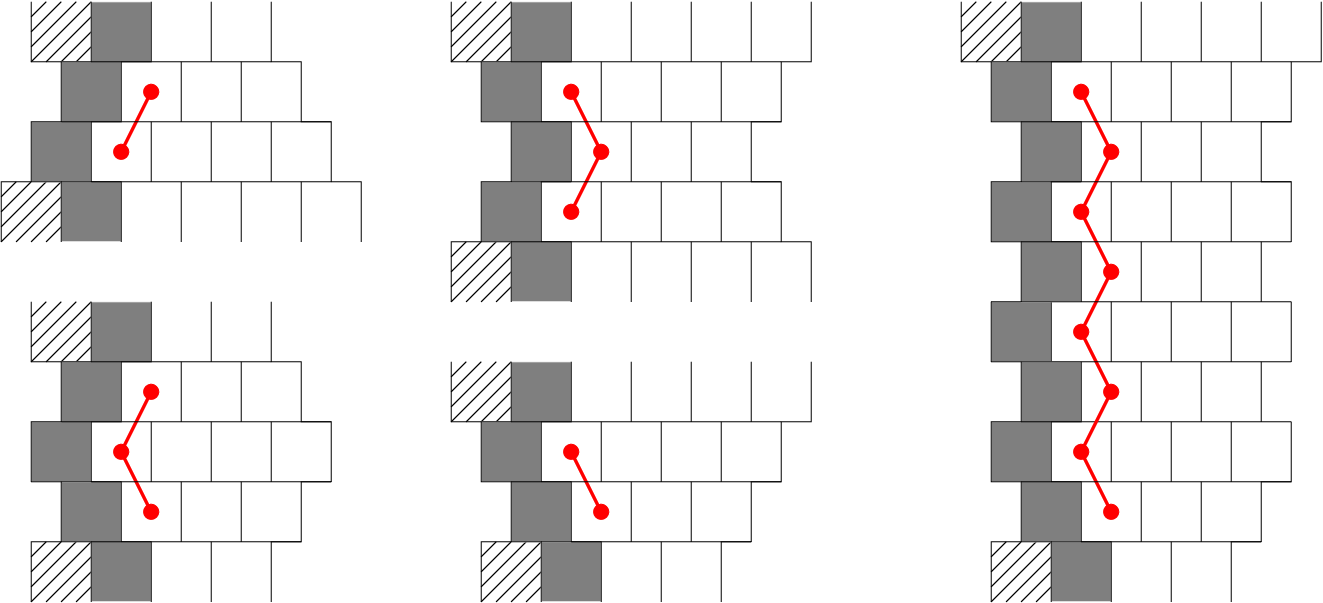
At this point we have identified a certain set of configurations that does belong to , but
does not belong to . However, we have to make a final step before we can identify all configurations
in with tiling configurations. This is due to the fact that certain parts of configurations seem to
belong to , but they do not respect the boundary conditions. Note that, at this point, we have reduced
all possible motifs to the following set:
””
””
””
””
which can be separated by single insertions of the motifs:
””
””
all modulo insertions of three dots and three zeroes along an entire column. Each
of the four basis motifs, comes with two directions, determined by whether the boundaries between the grey
and white segments follows the direction or .
Definition 4.
We assign a letter to each of the four basis motifs:
””
””
””
””
where the subscript is 1 or 2 when the direction of the motif is or respectively.
Note that the direction of a motif is not defined if neither the motif directly above it nor the motif directly below it is the same. We will start, however, by considering cases in which this does not happen. At the end of step 4 we will encounter a case where this point needs some attention.
We now want to study whether a vertical sequence of a certain motif can be followed by a sequence of a different motif, eventually, with a insertion of one of the motifs with 3 zeroes: ”” or ””.
Example 7.
As an example let us start with a sequence of motif . This sequence could be followed by motifs , and . However, it cannot be followed by motif , because it would not belong to . Nor can it be followed by motifs or , because it would not belong to (see fig. 22).

Similarly we find the following:
- •
motif can only be followed by motif .
- •
motif can only be followed by motif .
- •
motif can be followed by motifs , and .
- •
motif can be followed by motifs , and .
- •
motif can only follow after motif .
- •
motif can only follow after motif .
Finally, we know from lemma’s 7 and 8 that grey and white columns cannot branch or have end points, since their width always oscillates between 1 and 2 modulo 3 or 2, 3 and 4 modulo 3 for the grey and white segments respectively. Consequently, grey and white columns may wind around the torus several times, but they will always close to form a loop.
Let us combine this observation with the rules we found for stacking motifs. Consider, for example, motif , which can be followed by motifs , and . However, motifs and can only be followed by and respectively. Consequently, if motif is followed by either of these two motifs, we can never fulfill the boundary conditions, because the column cannot be closed to form a loop. Thus configurations in which motif is followed by motifs and do not belong to . In this same spirit we obtain the following lemma.
Lemma 16.
For configurations that belong to the following holds:
- •
motif can only be followed by motif and vice versa.
- •
motif can only be followed by motif and vice versa.
- •
motif can only be followed by motif and vice versa.
- •
motif can only be followed by motif and vice versa.
For motifs and the width of the white segment does not change, thus the motif with direction 1 can follow directly below or above this same motif with direction 2. For the motifs and , however, there is an intermediate motif of the type ”” or ””. Which of the two can be determined via the ’tic-tac-toe’ procedure. If we read the motifs of the rows from top to bottom, we find that a sequence of motifs will be followed by ””, to be followed by a sequence of motifs. Then the motifs will be followed by ””, which is then to be followed by another sequence of motifs. On the other hand, a sequence of motifs will be followed by ””, followed directly by a sequence of motifs. Finally, the motifs will be followed by ””, followed directly by another sequence of motifs (see fig. 23). It is readily checked that any other choice gives a configuration that does belong to , but not to .

Step 4
We are now ready to make the identification with the tiles. For the four basis motifs through the identification is shown in figure 24 and through are identified with a tiling in figure 25. Note that to distinguish motif from , where or , one has to consider also the motif on the row above or below this motif. These motifs can be followed by an arbitrary threefold of zeroes. Let us define the motif ””. For this motif we can also distinguish a direction, because its boundary will follow the left-most boundary of the white segment it is attached to. From figures 24 and 25 it is clear that the motifs can be followed by motif , where the should be the same. For the motifs and there is an exception: when the motif above these motifs is ”” and ”” respectively, they are followed by and respectively.


There can also be insertions of multiples of three dots in the four basis motifs. How this translates into tilings is shown in figure 27. More precisely, note that each basis motif contains a dotted line, connecting two sites along the direction 1 (black) and equivalently, all basis motifs contain a dotted line with direction 2 (blue). An insertion of three dots in a basis motif corresponds to an insertion of two tiles, shown in figure 26, at this dotted line. Note that here we cannot easily write the motif of dots directly in the tiles, however, the mapping is still unambiguous.

Finally, we have the motifs ”” and ””. Which tilings these motifs correspond to depends on whether they occur between the motifs and or the motifs and . In fact, in the first case, ”” will correspond to the same sequence of tiles as and ”” to the same tiling as . Similarly, in the latter case, ”” and , on the one hand, and ”” and , on the other hand, correspond to the same tilings. For an example see figure 28.

With these identifications there is one ambiguity, but it is easily dealt with. If there is a column in which the motifs alternate indefinitely between ”” and ””, we cannot determine whether the motif ”” is of type or . The same happens when the motifs ”” and ”” alternate indefinitely: the motif ”” could be of type or . Note that if we choose to identify the first with and the second with , the corresponding tilings would be indistinguishable. This also happens when we choose and . So we conclude that we should either choose and or and . The ambiguity is thus lifted by simply deciding that we will always choose, say, and .
Finally, we note that again the number of fermions in a certain configuration is the same as the number of tiles in the corresponding tiling. For the four basis motifs and the motifs with 3 zeroes or 3 dots, this follows from the arguments in section 5.3.1. For the motifs ”” and ””, we should look at figure 28. If the motif ”” sits between motifs and , the number of fermions in these three rows is and the number of sites is 3 times the number of sites: . So 9 fermions on 39 sites. Compare this with the corresponding tiling: it contains 2 times 3 tiles of area 4 and once 3 tiles of area 5. So 9 tiles with total area 39. Similarly, if the motif ”” sits between motifs and , the number of fermions in these three rows is and the number of sites is . The corresponding tiling contains 2 times 3 tiles of area 5 and once 3 tiles of area 4. For the corners between motifs and the comparison is slightly more subtle. Following the same arguments as above, we find that in this case the number of fermions in the motifs ”” and ”” do not agree with the number tiles in the corresponding tiling. However, the discrepancy is minus one in one case and plus on in the other, and since the boundary conditions dictate that the number of ””-motifs equals the number of ””-motifs, the discrepancies exactly cancel.
Step 5
The final step concerns the small correction in equation (43). With the four basis motifs, horizontal insertions of multiples of three dots and three zeroes and vertical insertions of the motifs ”” and ””, we can represent all elements in . With the mappings given in the previous step, we find a corresponding tiling for each of these elements. On the other hand, each possible tiling can be constructed with the small sequences of tiles given in the previous step. Thus we find that for each possible tiling there is a corresponding element in . Furthermore, we found that the number of fermions and the number of tiles agree. So we find , that is, the number of elements in with fermions equals the number of tilings of the square lattice with tiles. However, there is a small discrepancy in this one-to-one relation for the configurations with all zeroes or all dots. For and , it is readily verified that these configurations contain fermions. In the following we will first compute the number of elements of that these configurations account for. We shall call this , where stands for anomalous. We will then compute , the number of tilings consisting only of the tiles that correspond to either all zeroes or all dots (see fig. 26). Combining these results we obtain . Finally, since we found a one-to-one correspondence between tilings and elements of for , theorem 1 will then be established with as in equation (1).
As we discussed in section 5.3.1 for , the configurations with all dots and all zeroes actually correspond to multiple elements of the cohomology if there is a multiple of 3 sites per row, that is if . This is a direct consequence of theorem 2, which says that a periodic chain with length has two ground states. In fact, these configurations account for elements each, where is the total number of rows or, equivalently, of chains. On the other hand, for with they each represent one element of the cohomology. So we find for and otherwise.
Now, let us look at the corresponding tilings. For with there is no corresponding tiling, thus there is a discrepancy of 2 between the number of tilings and the number of elements in the cohomology. That is for . For there are tilings corresponding to the configurations with all zeroes or all dots. Along the direction these tilings have periodicity 3. The periodicity in the other direction is more involved. Given the boundary condition the tiling makes steps in the direction and steps in the direction, in arbitrary order. However, because of the periodicity of 3 in the direction one can also end at , that is, steps in the direction and steps in the direction, again in arbitrary order. Thus we find
If we define , where , we can write as:
Repeating these steps times, such that , we find
For the last term we find
We now compare the expression for with the expression for the number of elements in the cohomology represented by the configurations with all zeroes and all dots, . For this is . So we finally find
Combining this with the result for with , this can be cast in the compact form of equation (1).
Acknowledgments
We would like to thank P. Fendley for discussions and J. Jonsson for suggested improvements of the manuscript.
References
- [1] P. Fendley, K. Schoutens, and J. de Boer, Phys. Rev. Lett. 90, 120402 (2003).
- [2] P. Fendley, B. Nienhuis and K. Schoutens, J. Phys. A 36, 12399 (2003).
- [3] M. Beccaria and G. F. De Angelis, Phys. Rev. Lett. 94, 100401 (2005).
- [4] P. Fendley, K. Schoutens, Phys. Rev. Lett. 95, 046403 (2005).
- [5] H. van Eerten, J. Math. Phys. 46, 123302 (2005).
- [6] L. Huijse, K. Schoutens, Eur. Phys. J. B 64, 543-550 (2008).
- [7] L. Huijse, J. Halverson, P. Fendley, K. Schoutens, Phys. Rev. Lett. 101, 146406 (2008).
- [8] J. Jonsson, Electr. J. Comb. 13(1), #R67 (2006).
- [9] J. Jonsson, Certain Homology Cycles of the Independence Complex of Grid Graphs, Preprint (2005).
- [10] J. Jonsson, Hard Squares on Grids With Diagonal Boundary Conditions, Preprint (2006).
- [11] R.J. Baxter, Hard Squares for z=-1, preprint (2007).
- [12] M. Bousquet-Melou, S. Linusson, E. Nevo, J. Alg. Comb. 27, 423-450 (2008).
- [13] A. Engström, Eur. J. Comb. 30(2), 429-438 (2009).
- [14] P. Csorba, Electr. J. Comb. 16(2), #R11 (2009).
- [15] P. Fendley, K. Schoutens and H. van Eerten, J. Phys. A 38, 315 (2005).
- [16] R. Bott and L.W. Tu, Differential Forms in Algebraic Topology, GTM 82, (Springer Verlag, New York, 1982).
- [17] E. Witten, Nucl. Phys. B 202, 253 (1982).
- [18] R.J. Baxter, J. Phys. A: Math. Gen. 13, L61-L70 (1980).